Non-Destructive Evaluation of Reinforced Concrete Structures with Magnetic Flux Leakage and Eddy Current Methods—Comparative Analysis

Abstract

This article evaluates two essential non-destructive electromagnetic techniques, magnetic flux leakage (MFL) and eddy current (EC) methods, and their effectiveness in assessing the basic parameters of reinforced concrete (RC). The study compares both systems’ hardware and software components, emphasizing the adaptations implemented to tailor the methods for evaluating RC structures. Subsequently, the measurement results are analyzed, and association rules are extracted to demonstrate the relationships between variations in the physical parameters of the tested structure and the features of the measured waveforms. Finally, similar identification models are implemented, and the obtained identification results are compared. The paper documents and details all phases of this research. The findings indicate that while the operational principles of both methods are similar, the techniques differ significantly in terms of their measurement systems’ complexity and usability. The eddy current (EC) method exhibits superior spatial resolution, whereas the magnetic method is more straightforward and offers a greater effective range and favorable association rules. Consequently, it is recommended that both techniques be utilized for different structures and in varying contexts. The techniques’ advantages, disadvantages, and limitations are discussed in this work and supported by the measurement results.

1. Introduction

1.1. Motivation

This paper compares the two most promising NDT methods for evaluating the basic parameters of reinforced concrete (RC) structures. Such evaluation is needed for acceptance tests or to determine the physical properties of old objects whose basic parameters are unknown.

RC has been used as a primary construction material for over a century. Hundreds of millions of reinforced concrete (RC) structures of various types and sizes have been built globally during this time. Identifying fundamental parameters in these structures is crucial for investors and construction inspectors. The acceptance tests ensure that the structural parameters and materials meet design specifications. Usually, investigations of this kind include the evaluation of parameters like concrete cover thickness (h), rebar diameter (D), and the class of steel (ductility and hardness of the alloy [1]). Nowadays, acceptance tests are mainly conducted using destructive testing methods. The concrete cover is removed during the investigation, and the materials are evaluated visually [2,3,4,5].

Additionally, the parameters can be evaluated on existing structures before renovation or modernization works (if documents are lost and the structure specification needs to be discovered). Knowledge about the materials used is essential, for example, to calculate the structure’s load-bearing capacity and determine whether proposed changes are feasible and safe [2,3].

Due to the worldwide scale effect (the number of RC structures), such tests have enormous practical importance. Substituting destructive techniques with nondestructive testing (NDT) methods would greatly expedite the testing process and enable reductions in the associated costs. These advancements could increase the prevalence of such tests, ultimately improving overall safety by ensuring the use of materials in accordance with the project. Therefore, developing innovative nondestructive testing (NDT) methods tailored explicitly for inspecting reinforced concrete (RC) structures is a critical concern.

The direct nondestructive evaluation of reinforcing bars is mainly achievable through electromagnetic and specific mechanical techniques. However, only electromagnetic methods are specifically designed for assessing metal components (such as rebars), while mechanical methods offer greater versatility. Electromagnetic techniques facilitate direct interaction with rebar, reducing interference and attenuation from the surrounding concrete cover. Among these methods, the eddy current (EC) technique is the preferred option for assessing reinforced concrete (RC) structures. However, the magnetic method presents a solid alternative to EC. Recent advancements in magnetic sensor technology have significantly increased the popularity of such systems in various nondestructive testing (NDT) applications. Magnetic flux leakage (MFL) is the most promising among the different magnetic methods [6].

This paper offers a comparative analysis of the eddy current (EC) method and the magnetic flux leakage (MFL) approach. Both techniques have been adapted for evaluating RC structures and compared regarding system complexity, spatial resolution, effective range, and simplicity of basic RC structure parameter identification.

1.2. Non-Destructive Methods for Testing Concrete Structures

Nondestructive testing (NDT) methods fulfill two roles: they can function as preliminary techniques before semi-destructive or destructive testing or as primary diagnostic tools. Various NDT methods can assess reinforced concrete (RC) structures. Some methods are designed explicitly for evaluating concrete [7,8,9], while others focus solely on testing the reinforcement mesh. Additionally, some techniques assess the entire structure comprehensively.

The RC structure parameters that can be evaluated using NDT methods include:

1.

Visual condition of concrete—the category is represented by the oldest NDT method: visual inspection (VI).

2.

Evaluation of electromagnetic properties—this approach offers several advantages, including direct interaction with the reinforcement, minimal attenuation of electromagnetic waves by concrete, cost-effectiveness, and a broad range of operational principles and applications. This category can be further divided into three subcategories:

a.

Magnetic properties—this category encompasses passive methods, such as the residual magnetization technique (RMT), and active methods where the object being tested is continuously magnetized, as seen in magnetic flux leakage (MFL), or magnetized before testing, as in magnetic particle inspection (MPI) [4,5,6];

b.

AC electromagnetic induction—this category is represented by the eddy current (EC) method [4,5,6];

c.

Reflection of electromagnetic waves—this subcategory is represented by ground-penetrating radar (GPR) [10,11,12,13];

3.

Density of components in RC structure—this category is represented by radiography (X-ray) [4,5,14].

4.

Carbonation level of concrete—providing insights into the risk of corrosion of the carbonation mechanism (the connection between corrosion and carbonation is described in [12]); this parameter can be evaluated using three different properties:

a.

Electrical properties—this category includes the half-cell potential method (HCP) and concrete resistivity method (CR). The HCP technique assesses the capacity (electrochemical potential) between a reference electrode placed on the structure surface and reinforcement placed inside the structure [15,16]. The CR is used to measure the electrical resistivity of concrete [17,18,19]. Both electrical properties change while the carbonation process progresses;

b.

pH (chemical tests)—the rainbow test (RT) and phenolphthalein test (PT) fall within this category, allowing for the assessment of carbonation depth through the measurement of concrete pH levels [20,21];

c.

Strength of the concrete—this category of methods includes the Schmidt hammer (SH) and Windsor probe (WP). Both methods test concrete by hitting the surface and measuring the outcome of the impact [20,21].

5.

Thermal properties of the whole structure—infrared thermography (IR) enables exploration of the difference between the thermal properties of concrete and steel by monitoring the heating and cooling processes of the RC structure [22,23,24].

6.

Mechanical properties of the whole structure—the methods test propagation of mechanical waves (sonic and ultrasonic frequencies)—waves may be generated by the tested object (passive method), like in the case of acoustic emission (AE) [25,26], by induced electromagnetic waves, like in the case of electromagnetic acoustic transduction (EMAT), or by mechanical wave—impact echo (IE) and most forms of ultrasonic testing (UT) [27,28,29,30,31].

7.

Natural frequencies of the whole structure (low frequency)—the methods in this category investigate the resonance frequencies of the object. Vibrations can be induced by electromagnetic waves (as seen in the M5 system), physical impact (such as in the hammer impact test (HIT)), or passively through vibration monitoring (VM). Modal analysis is frequently employed in this type of testing [6,32,33].

Another approach to categorizing NDT methods employed in the diagnostics of reinforced concrete (RC) structures is based on their operational principles. Table 1 presents a classification of the methods, comparing them across several criteria:

• Evaluation of rebars: this category assesses the capability to locate reinforcing bars and identify their class and diameter within typical concrete cover thickness ranges (20–50 mm).
• Evaluation of corrosion: this category evaluates the ability to detect corrosion by examining delamination and diameter reduction, focusing on standard concrete cover thickness ranges.
• Evaluation of h (concrete cover thickness): this criterion measures the method’s effectiveness in estimating the thickness of the concrete cover within typical ranges.
• Evaluation of carbonation: this category involves analyzing various changes in the physical properties of concrete that indicate ongoing carbonation processes.
• Evaluation of concrete: this category serves to assess concrete integrity. The criterion includes the detection of delamination, large air voids, macro heterogeneities, and cracks within the concrete.
• Area testing (spatial measurement capability): this category highlights the method’s ability to conduct measurements simultaneously at many points (creating a measurement matrix).
• Commercial viability: this criterion evaluates the method’s usability for commercial applications, including cost measurements and any technical limitations that may affect its utility.

Table 1. The capability of the NDT methods to RC structure evaluation.

Category		Example Methods		Evaluation of:						Area Testing	Commercial Viability
				Rebar	Corrosion	h	Carbonation	Concrete
Mechanical
low frequency		M5 1, HIT 2, VM 3
sonic		IE 4, AE 5
ultrasonic		UT 6
Magnetic
active		MFL 7, MPI 8
passive		RM 9
Electric
capacity		HCP 10
resistance		CR 11
Electromagnetic
low frequency		MFL 7
medium frequency		EC 12
microwave		GPR 13
terahertz		-
infrared		IR 14
visible		VI 15
visible		FO 16
radiography		X-ray
Chemical		RT 17, PT 18
Concrete strength		WP 19, SH 20
	not suitable		suitable in some cases				moderate suitable			well suitable

¹ M5—Magnetic Force Induced Vibration Evaluation (MFIVE); ² HIT—Hammer Impact Test; ³ VM—Vibration Monitoring; ⁴ IE—Impact Echo; ⁵ AE—Acoustic Emission; ⁶ UT—Ultrasonic Testing; ⁷ MFL—Magnetic Flux Leakage; ⁸ MPI—Magnetic Particle Inspection; ⁹ RM—Residual Magnetization; ¹⁰ HCP—Half-Cell Potential; ¹¹ CR—Concrete Resistivity; ¹² EC—Eddy Current; ¹³ GPR—Ground Penetrating Radar; ¹⁴ IR—Infrared Radiation (Thermography); ¹⁵ VI—Visual Inspection; ¹⁶ FO—Fiber Optic; ¹⁷ RT—Rainbow Test; ¹⁸ PT—Phenolphthalein Test; ¹⁹ WP—Windsor Probe; ²⁰ SH—Schmidt Hammer.

Table 1. The capability of the NDT methods to RC structure evaluation.

Category		Example Methods		Evaluation of:						Area Testing	Commercial Viability
				Rebar	Corrosion	h	Carbonation	Concrete
Mechanical
low frequency		M5 1, HIT 2, VM 3
sonic		IE 4, AE 5
ultrasonic		UT 6
Magnetic
active		MFL 7, MPI 8
passive		RM 9
Electric
capacity		HCP 10
resistance		CR 11
Electromagnetic
low frequency		MFL 7
medium frequency		EC 12
microwave		GPR 13
terahertz		-
infrared		IR 14
visible		VI 15
visible		FO 16
radiography		X-ray
Chemical		RT 17, PT 18
Concrete strength		WP 19, SH 20
	not suitable		suitable in some cases				moderate suitable			well suitable

¹ M5—Magnetic Force Induced Vibration Evaluation (MFIVE); ² HIT—Hammer Impact Test; ³ VM—Vibration Monitoring; ⁴ IE—Impact Echo; ⁵ AE—Acoustic Emission; ⁶ UT—Ultrasonic Testing; ⁷ MFL—Magnetic Flux Leakage; ⁸ MPI—Magnetic Particle Inspection; ⁹ RM—Residual Magnetization; ¹⁰ HCP—Half-Cell Potential; ¹¹ CR—Concrete Resistivity; ¹² EC—Eddy Current; ¹³ GPR—Ground Penetrating Radar; ¹⁴ IR—Infrared Radiation (Thermography); ¹⁵ VI—Visual Inspection; ¹⁶ FO—Fiber Optic; ¹⁷ RT—Rainbow Test; ¹⁸ PT—Phenolphthalein Test; ¹⁹ WP—Windsor Probe; ²⁰ SH—Schmidt Hammer.

The analysis in Table 1 indicates that the range of NDT methods applicable to examining reinforced meshes is limited.

Radiography is highly effective, designed for area testing, and the obtained results are relatively easy to interpret. However, the technique has several significant limitations. Typically, both the source and detector must be positioned on opposite sides of the object, which can complicate the testing process or make it impossible in many instances. Additionally, this method causes health risks to personnel and is relatively costly, rendering it impractical for most applications [4,5,14].

Ground-penetrating radar (GPR) enables the detection of rebar from several centimeters to over ten meters, significantly exceeding the maximum detection range of the eddy current (EC) and magnetic flux leakage (MFL) methods (which are limited mainly to less than 200 mm). GPR is particularly effective (and primarily used) for rapid area assessments. However, the interpretation of the results can be challenging. The accuracy of the method is limited. Additionally, this method is unsuitable (in most cases) for typical concrete cover thicknesses (which are too low for radar), limiting its practical application. Furthermore, GPR equipment costs are high [10,11,12,13].

In many cases, ultrasonic testing (UT) can be a viable alternative to eddy current (EC) and magnetic flux leakage (MFL) methods. UT is versatile, capable of locating reinforcing bars, evaluating their parameters, and sometimes detecting corrosion. Additionally, it can be used for area testing, such as with the total focusing method. Specific variants of UT can effectively assess concrete cover thicknesses greater than 0.5 m. However, UT methods were primarily designed for evaluating concrete, which means that various factors can affect the results and complicate the identification process. Moreover, the equipment needed for UT tends to be relatively expensive, and the method generally provides lower accuracy in rebar identification compared to EC and MFL [27,28,29,30,31].

Both eddy current (EC) and magnetic flux leakage (MFL) methods are well-suited for evaluating reinforcing bars in reinforced concrete (RC) structures. Concrete is practically transparent to electromagnetic waves (magnetic permeability is similar to air permeability). This makes direct interaction with the rebar possible with minimal damping. Both techniques prove effective within 0 to 60 mm (a range higher than typical concrete cover thickness). The EC method can reliably detect the presence of reinforcing bars, determine their distance from the sensor (indicative of concrete cover thickness), and assess their position, diameter, and steel grade [34,35,36,37,38,39]. Similarly, the MFL method has been utilized to measure concrete cover thickness [40,41,42,43], determine the diameter of reinforcing bars [40,43], and classify the class of rebar steel [40,41]. However, achieving simultaneous identification of all three elemental parameters (concrete cover thickness (h), diameter (D), and steel class) using this method has posed significant challenges so far. Nonetheless, recent investigations show that it is possible [44]. Moreover, both EC [45,46,47] and MFL [48,49,50,51,52] methods can, in some cases, detect corrosion. In contrast to EC, the MFL method can also be utilized for area testing [6] and mapping reinforcement grids [42,43,44,45,46,47,48,49,50,51,52,53,54,55].

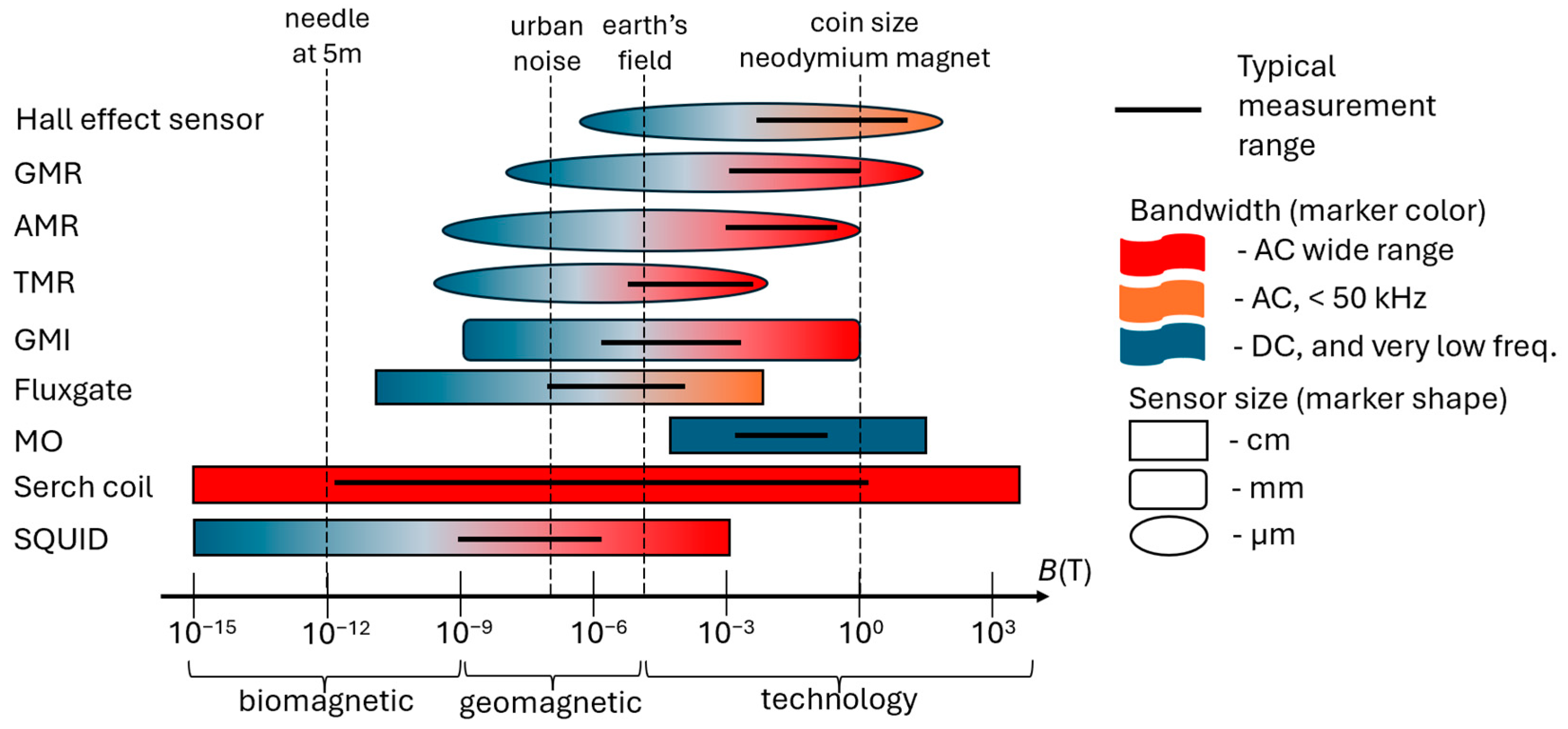
1.3. Selection of the Magnetic Sensor

The literature review indicates that the magnetic flux leakage (MFL) method provides advantages over eddy current (EC) in conducting area tests and facilitating the mapping of reinforcement mesh. However, effective mapping of the reinforcement mesh necessitates the selection of appropriate sensors suitable for the area transducer. An analysis of commercially available elements is conducted in [41]. Sensitivity, size, and bandwidth were chosen as critical selection criteria. A summary of the values for these three parameters is presented in Figure 1.

The magnetic transducer is designed to operate in the range of 1 to 10 mT—suitable for applications within this magnetic field range (Figure 1). The sensors must enable measurements of the DC magnetic field and be as compact as possible. The technologies that best meet these criteria are GMR, AMR, and MO. The MO sensor system was previously designed, constructed, and tested; results are presented in [56].

In the case of an eddy current (EC) transducer, the measurement range should match that of the magnetic flux leakage (MFL) method. The required bandwidth is a minimum of 50 kHz, with no specific size limitations. The technologies that best meet these criteria include GMR, AMR, and search coils.

2. Measuring Systems, Materials and Methods

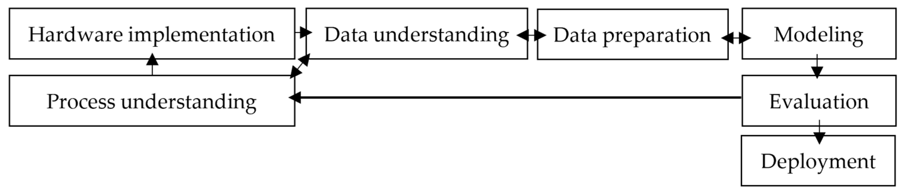
2.1. Methodology

The comprehensive research methodology was originally detailed in [44].

Knowledge acquisition from measurements obtained through non-destructive testing (NDT) can be conducted according to an algorithm similar to the classic CRISP-DM model (Cross-Industry Standard Process for Data Mining). The CRISP-DM framework is an iterative process consisting of seven steps and some feedback loops [56].

The first step is to thoroughly understand the problem and the physical phenomena related to the utilized NDT method. This phase includes an extensive literature review and simulation studies. The simulations employed the finite element method using the commercial software COMSOL v6.0. These tests are designed to assess the theoretically developed concepts and to create preliminary versions of the laboratory system. An additional critical role of the simulations is to provide data that can be utilized to verify and validate the measurement results obtained.

The subsequent step involves the preparation of samples and the configuration of the measurement systems.

In the next step, data are obtained and interpreted. During this phase, measurements are conducted by moving the sensor over the sample perpendicularly to the tested reinforcing bar. In the case of the eddy current method, both the sensor and the excitation are moved together. Conversely, only the sensor is moved for the magnetic method while the excitation system remains positioned directly above the reinforcing bar. Next, attributes representing waveforms are defined and utilized to extract association rules. The rules link variations in the waveform to corresponding changes in the adequate sample physical parameters. Association rules are derived using visualization techniques, statistical analyses, and specialized algorithms. Additionally, the measurement results are compared with simulation data at this stage. Preliminary analyses often indicate the need for adjustments to the laboratory setup and may necessitate repeated measurements, frequently requiring multiple iterations.

In the third step, data preparation is conducted to enable effective identification through machine learning. This process may include outlier removal, normalization, quantization, discretization, and curve smoothing.

The modeling stage focuses on developing the identification model. During this phase, attributes are processed and selected. Techniques such as aggregation, filtering, wrappers, and more advanced methods like rough set theory or principal component analysis (PCA) can be employed during the process. Then, various classifiers and identification algorithms are tested to select the best method.

The subsequent stage is evaluation. This step is intended to address any remaining uncertainties and validate the suitability of particular solutions and configurations. If the model receives a negative assessment, it will require a thorough re-evaluation of all prior stages.

The final step involves model deployment. During this phase, real objects with unknown parameters are tested.

Figure 2 illustrates the sequential stages of knowledge acquisition and the most frequently encountered feedback loops inherent to this model, which has been adapted to the specifics of NDT.

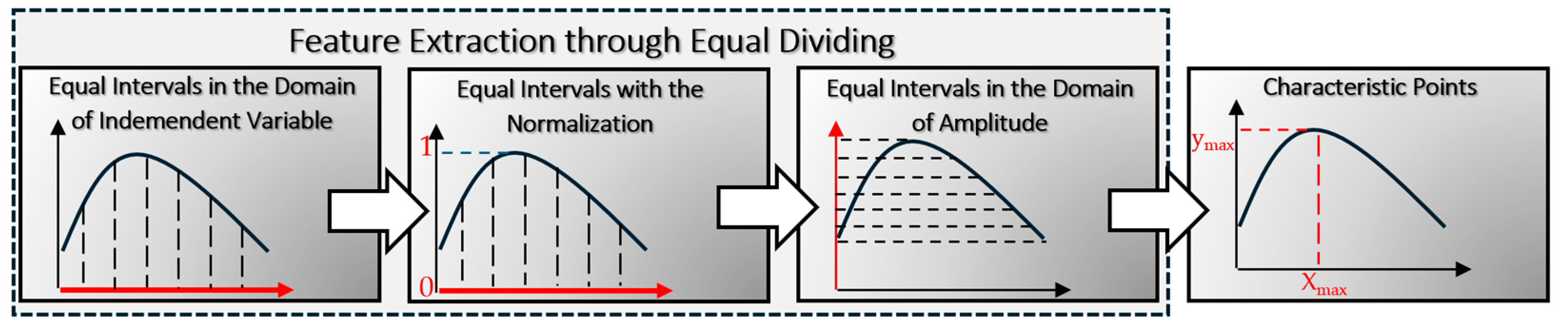
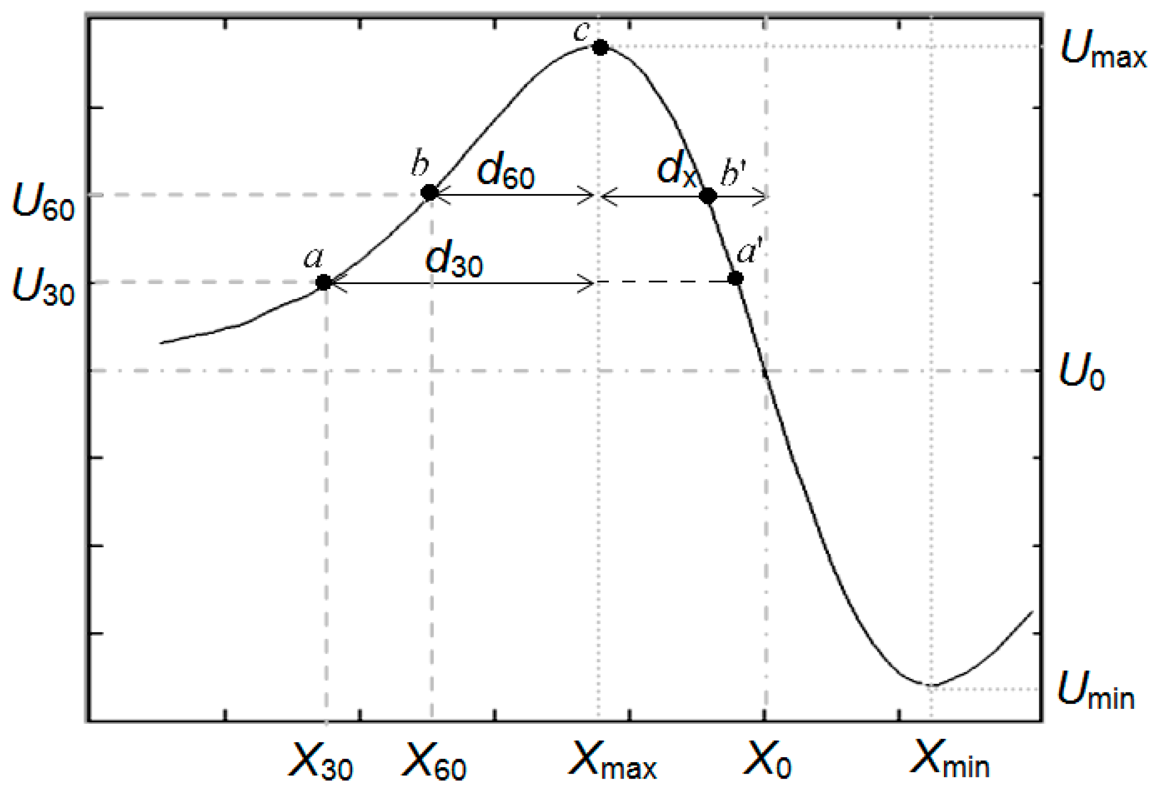
2.1.1. Feature Extraction

Studies on magnetic and eddy current methods [34,40,44] have shown that simultaneously identifying three parameters from the same dataset presents a significant challenge. The effectiveness of the identification largely depends on the feature extraction techniques employed to characterize the waveform attributes. In the process of attribute extraction, it is crucial to consider specific conditions and limitations, including:

• The number of attributes used in the model should be kept to a minimum to reduce the impact of the curse of dimensionality;
• The attributes should be independent and demonstrate low correlation with each other. When attributes are dependent or exhibit high correlation, they can exacerbate the curse of dimensionality without providing meaningful knowledge;
• The attributes included in the model must accurately represent the shape and characteristics of the measured waveforms.

The study of attribute extraction is performed iteratively, adhering to the methodology described in [44]. Each subsequent method is developed based on enhancements from earlier versions. Each one presents unique strengths, limitations, and weaknesses. Figure 3 presents the development of these methods.

Dividing the domain of the independent variable into equal intervals is an elemental method for extracting features from the waveform. Attributes are created by saving amplitude values (attributes) for subsequent positions (equally spaced from each other) on the independent variable. The positions are evenly spaced apart. While the method is straightforward, many attributes are needed to reflect the waveform’s shape accurately.

Experiments have demonstrated that treating amplitude as an individual feature can significantly enhance identification accuracy. In these instances, shape attributes are derived from the normalized waveform and separated from the amplitude value. This approach is referred to as equal intervals with normalization.

In the following research phase, the extraction method for the shape attributes is enhanced. The technique is called equal intervals in the amplitude domain. This method involves dividing the vertical axis into equal intervals. The sampling frequency of attributes is proportional to the derivative of the waveform and increases in areas where the waveform rises more steeply. This modification enables a more precise depiction of the waveform’s shape using fewer attributes. However, if the tested waveform is not monotonic, multiple abscissa values can be assigned to a single amplitude value.

The primary benefit of all three feature extraction methods through equal dividing is the ability to extract attributes without requiring initial knowledge or testing the association rules between waveforms and structure physical parameters. Prior understanding of the studied process is also not necessary. This makes these techniques highly universal and applicable in most contexts. The methods can be utilized as an intermediate step in the development (e.g., before using the characteristic point method to define characteristic points).

On the other hand, a notable drawback of these methods is the necessity to extract many features to capture the shape of the waveform. This causes problems connected to the curse of dimensionality. As the number of features grows, the required number of records (database size) should increase exponentially. Moreover, obtained shape attributes are usually highly correlated. As a result, it is essential to reduce the number of features (usually, the number of attributes should be smaller than five). The reduction process requires time, experience, and knowledge about the tools that can be used (filtering, aggregation, wrappers, principal component analysis, rough set theory [57,58], etc.).

Attribute identification and selection require balancing the need to minimize the number of features (reduction) and effectively represent the waveform shape. The characteristic points method can minimize or remove the need for attribute reduction. The technique involves the arbitrary selection of features that vary with changes in the studied object (e.g., extrema, inflection points of the waveform, coordinates of these points, or offset). The technique requires some initial knowledge, which can be gathered from association rules, statistical and mathematical analyses, simulations, or a general understanding of the process. The schematic process of attribute extraction is presented in Figure 4.

This investigation applies the equal intervals in the domain of amplitude method as the first step. Each waveform’s amplitude is divided into equal intervals, with each interval accounting for 5% of the amplitude. Consequently, sections are designated as, e.g., U₃₀ for 30%, U₆₀ for 60%, and U_max for 100% of the maximum amplitude (Figure 5).

Subsequently, the points corresponding to the U values are marked on the graph (point a for U₃₀, b for U₆₀, c for U_max) and projected onto the abscissa axis. This led to the creation of new variables: X₃₀, X₆₀, and X_max. These variables are next used to determine the shape attributes d₃₀, d₆₀, and d_x.

It can be noted that for each value marked on the ordinate axis (except U_max), two corresponding values can be read on the abscissa axis: one smaller than X_max (a and b) and one larger than X_max (a’ and b’). The attribute d_x, representing the distance between the coordinate of the zero value (X₀) and the maximum value (X_max) is calculated to address this issue. Subsequently, X_max is used as the reference point for the other shape attributes instead of X₀.

Furthermore, parameters such as amplitude and offset are established. Figure 6 illustrates the definitions of these terms.

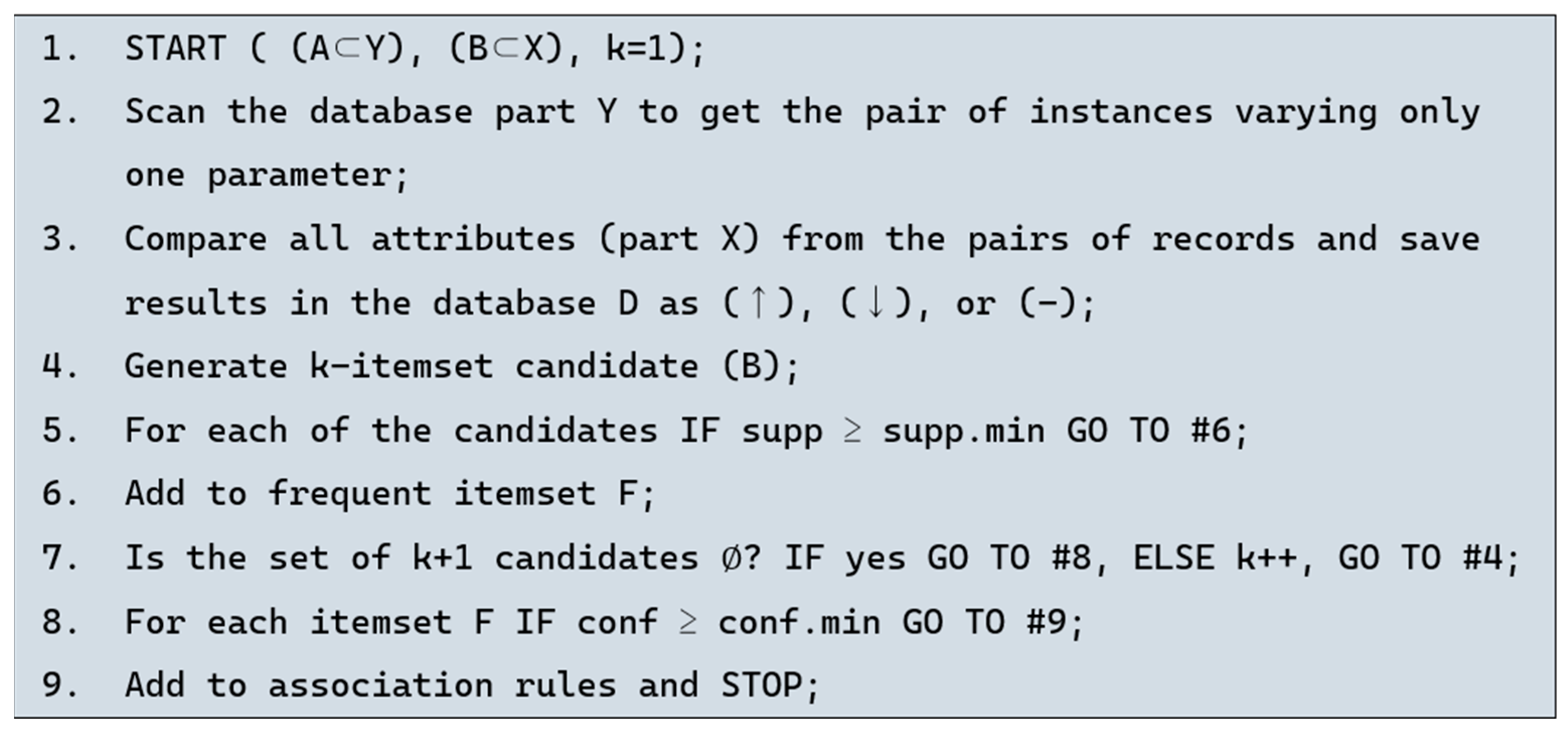
2.1.2. Extraction of Association Rules

Exploring the relationships between the physical parameters of a structure and the waveform features obtained from NDT investigations is a difficult-to-standardize process. Various analytical methods can be employed to understand the association rules better and obtain the initial knowledge (Figure 4) necessary for further investigation. Algorithms for extracting association rules, such as Apriori, can be advantageous. The large number of features generated through equal division methods allows for a more in-depth analysis of these relationships, improving the understanding of the underlying processes and creating an effective classification algorithm [59,60,61,62,63].

Unlike methods such as rough set theory, association rule extraction techniques are not employed for classification purposes (matching sets of predictors to specific values of the decision variable). The main objective of these algorithms is to demonstrate how changes in a physical parameter (such as an increase in cover thickness) will influence the waveform. However, similar to rough set theory, the method can be utilized for attribute selection. The initial step in exploring association rules during non-destructive testing (NDT) investigations involves constructing a database containing comparisons of original records. The compared records can differ by only one structural parameter, representing the smallest possible change. The compared parameters (both structure and waveform) can be categorized as increase (↑), decrease (↓), or no change (-). Finally, a rule can be formulated as follows (1):

If (BODY), then (HEAD) [support, confidence]

(1)

where:

BODY (A) is a change in a specific parameter of the structure;

HEAD (B) is a change in a specific parameter of the waveform.

The strength of the rule is assessed using two indicators: support and confidence.

Support is a ratio of the number of records in which the rule is present to the total number of records in the database (D). This indicator is given as (2):

$$\mathrm{supp} (\mathrm{A})={\displaystyle \frac{\#\left\{{\mathrm{d}}_{\mathrm{i}}\in \mathrm{D}:\mathrm{A}\subset {\mathrm{d}}_{\mathrm{i}}\right\}}{\#\mathrm{D}}}\approx \mathrm{P}(\mathrm{A})$$

(2)

The confidence indicator is a conditional probability that the entire rule will be observed, contingent upon the presence of the BODY (A). This indicator is given as (3):

$$\mathrm{conf}\left(\mathrm{A}\to \mathrm{B}\right)={\displaystyle \frac{\mathrm{supp} (\mathrm{A}\cup \mathrm{B})}{\mathrm{supp} \left(\mathrm{A}\right)}}\approx \mathrm{P}(\mathrm{B}|\mathrm{A})$$

(3)

The proposed method for discovering association rules closely resembles the traditional Apriori algorithm [59,60,61,62,63]. This approach is founded on the principle that significant rules are derived solely from frequent item sets. Such item sets must surpass the minimum support and confidence thresholds established by the investigator. In comparison to the classical algorithm, a few significant changes have been introduced:

• Set A includes only the structure’s physical parameters;
• Set B includes only the waveform’s parameters;
• The BODY length equals 1; only one physical parameter (A) can change.

The introduced modifications improve the algorithm’s efficiency by reducing the search space for association rules.

The algorithm of the designed method is shown in Figure 7.

2.2. Measuring System and Samples

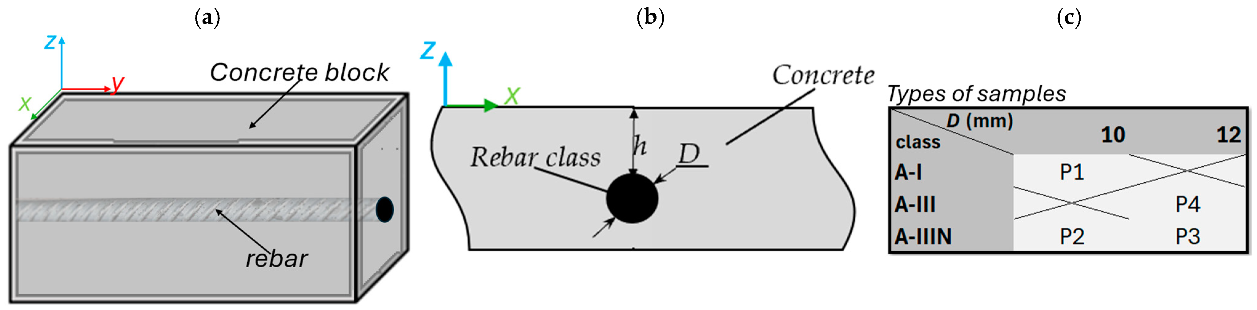
2.2.1. Samples

Figure 8 displays a schematic representation of the sample along with its parameters.

RC structures are defined by three key parameters: concrete cover thickness (h), rebar diameter (D), and class of reinforced steel. The class parameter indicates the ductility and strength of the alloy. Class A-I has the highest strength and lowest ductility, while A-IIIN has the lowest strength and highest ductility [1].

The main tests are conducted on samples P1–P4 (Figure 8c). Each measurement is repeated a minimum of ten times. To further explore and validate the results from the main tests, supplementary measurements are performed using the eddy current (EC) method. The additional tests are mostly used to explore how the size of the EC transducer affects the outcomes and more accurately investigate association rules connected to the diameter (D) and thickness of the concrete cover (h) identification. The rebars used during supplementary measurements are presented in Figure 9.

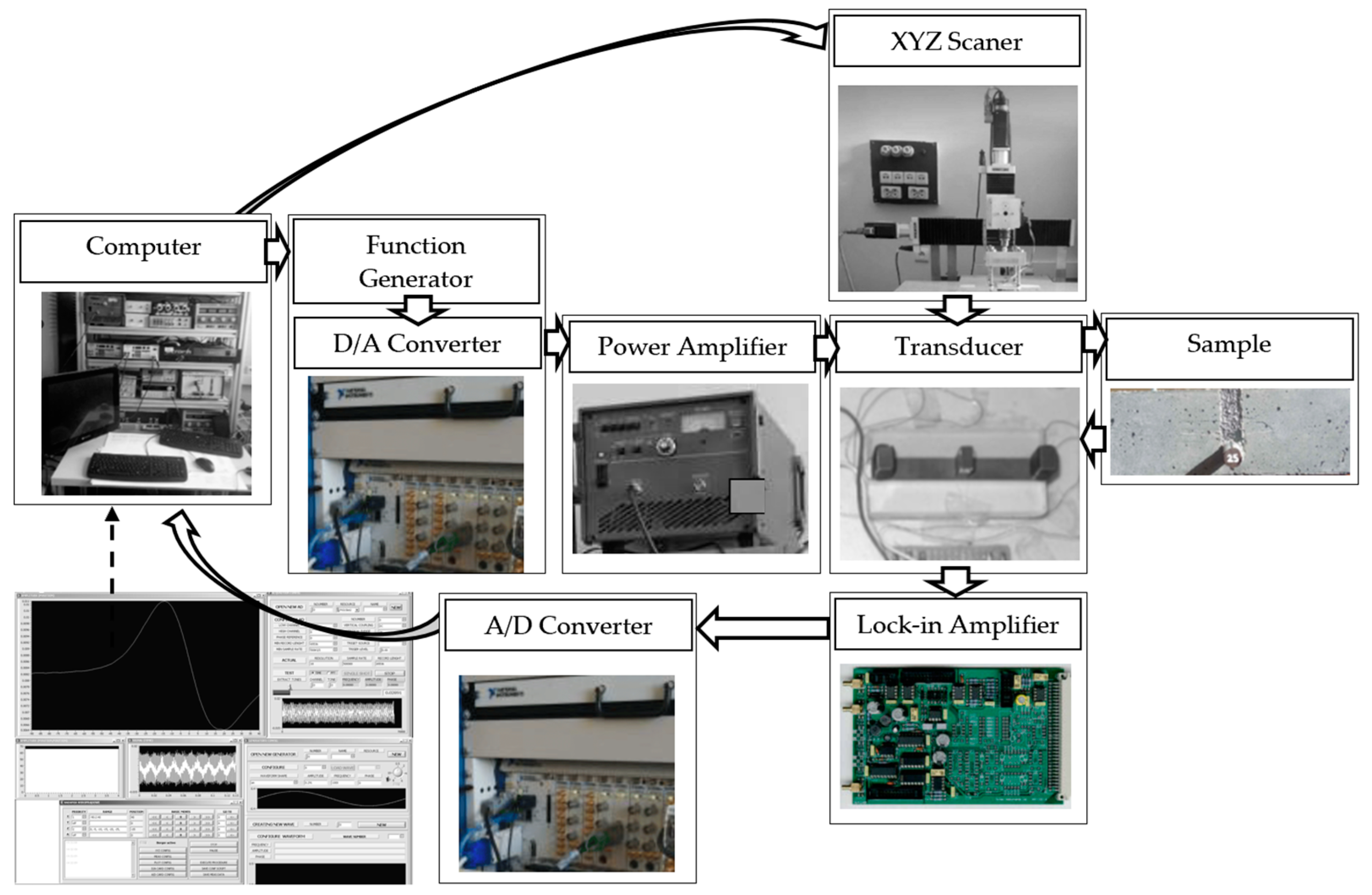
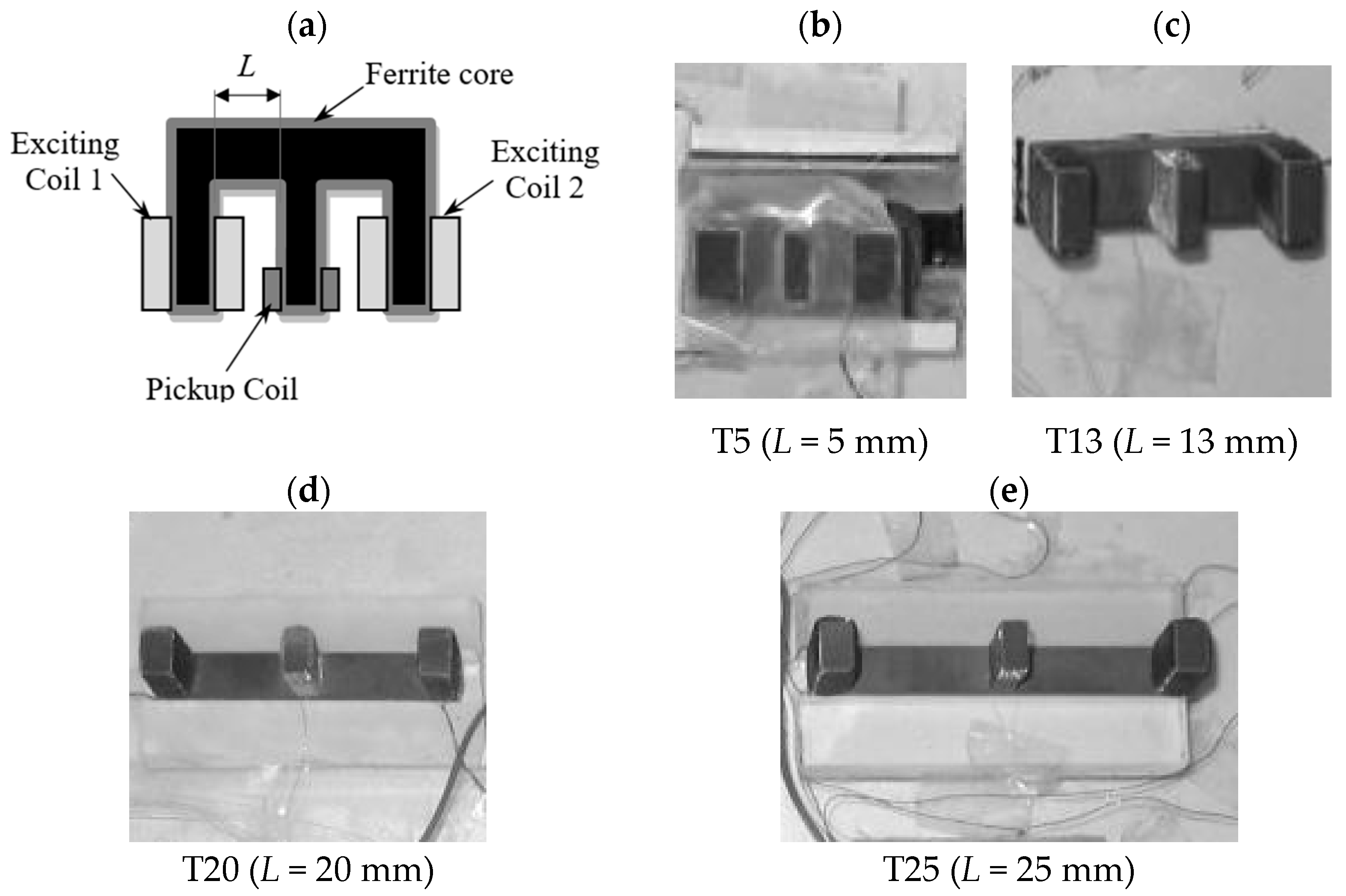
2.2.2. Comparison of Measuring Systems

Figure 10 illustrates the block diagram of the eddy current (EC) system, while Figure 11 depicts the corresponding magnetic flux leakage (MFL) system.

The eddy current (EC) system comprises an E-shaped transducer and four subsystems: an XYZ scanner, an excitation subsystem, a data acquisition subsystem, and a control computer. The control computer generates the excitation signal using LabVIEW and a data acquisition card (DAC), which converts a digital signal to an analog. This signal is sent to the acoustic amplifier and, from there, to the transducer’s excitation coils. In the experiments, four transducers were used (Figure 11).

When a reinforcing bar is near the transducer, the magnetic field generated by the excitation coils (as described by Ampere’s law) induces eddy currents within the rebar. According to Lenz’s law, these currents produce an additional magnetic field that opposes the primary field. The interaction of all these fields affects the pick-up coil, leading to the induced voltage (pick-up coil).

When the transducer is located considerably far from the reinforcement, the signal obtained from the receiving coil tends to be weak and noisy. However, since the signal’s frequency is known (equal to the frequency of the excitation signal), it can be effectively separated from the noise using a lock-in amplifier. The filtered signal is then directed through the A/D converter to the computer for further analysis. Typically, additional filtering with a Butterworth filter is necessary.

The measuring robot moves the transducer perpendicularly to the reinforcing bar, enabling the measurement waveform to be recorded from the receiving coil.

The magnetic fields generated by the excitation coils can either overlap (absolute transducer) or cancel each other out (differential transducer). Examples of both absolute and differential signals are illustrated in Figure 12.

A differential transducer is chosen for the investigations. While its signal-to-noise ratio (SNR) is comparable to that of an absolute transducer, it facilitates a much simpler identification of characteristic points (attributes such as X_max, X_min, d_x = X_max − X_o, etc.). Furthermore, it is less affected by interference generated by the measuring coils (X_r and X_s).

In designing an EC system, several key factors must be considered:

• Transducer size: a larger transducer size results in lower spatial resolution and higher effective range.
• Excitation frequency: a lower frequency results in lower spatial resolution and higher effective range.
• Magnetic induction (B).

The value of magnetic induction is influenced by the current flowing through the excitation coil (I), the number of turns (N), the magnetic permeability of the core (α), and the length of the winding wire (l), as described by Formula (4):

$$\overrightarrow{B}={\displaystyle \frac{I·N}{l}}·\mu$$

(4)

The magnitude of the current (following Ohm’s law (5)) is influenced by the voltage applied to the excitation coil (U), the reactance of the inductive impedance (X_L), and the resistance (R):

$$\left|I\right|={\displaystyle \frac{\left|U\right|}{\sqrt{R^2+X_L^2}}}$$

(5)

Resistance depends on the resistivity (ρ), the length of the winding (l), and the cross-sectional area of the winding (S). At the same time, reactance is influenced by the excitation frequency (f), the magnetic permeability of the core (α), the cross-sectional area of the core (A), the number of turns (N), and the length of the winding (l). Ultimately, the equation takes the form (6):

$$\left|I\right|={\displaystyle \frac{\left|U\right|}{\sqrt{{\left(\frac{\rho \cdot l}{S}\right)}^2+{\left(2\pi ·f·\frac{\mu \cdot N^2\cdot A}{l}\right)}^2}}}$$

(6)

EC systems are relatively complex (both in hardware and software), with many factors affecting the final result. Additionally, (since this is a surface method) the signals obtained from evaluating RC structures can be weak and noisy, especially when dealing with a thick concrete cover. Eddy current transducer excitation can be implemented in various ways, ranging from coils driven by single- or multi-frequency signals to pulsed excitation [64,65] or rotating magnets [66,67,68]. However, in all versions, the excitation is married to the pickup sensor, which poses challenges in densely reinforced RC objects. The interaction between neighboring reinforcing rebars may distort the measurements and result in incorrect classifications. Moreover, it also makes it more challenging to build an area testing system [34]. On the other hand, properties of systems of this kind are straightforward to regulate, and spatial resolution can be high (the EC method can identify defects that are approximately the size of a wavelength [69]).

The alternative for EC can be a magnetic system (Figure 13).

The main advantage of magnetic nondestructive testing systems is their straightforward design, which is typically much less complex than eddy current designs. The system presented in Figure 13 includes an excitation subsystem, a positioning robot, a magnetic field sensor (HMC5883L, Honeywell, NJ, USA [70]), and a data acquisition subsystem. Although the typical setup for MFL transducers and measurement procedures resembles that of EC, the authors argue that this configuration could be more optimal and requires significant adjustments. In the system, the following modifications have been implemented:

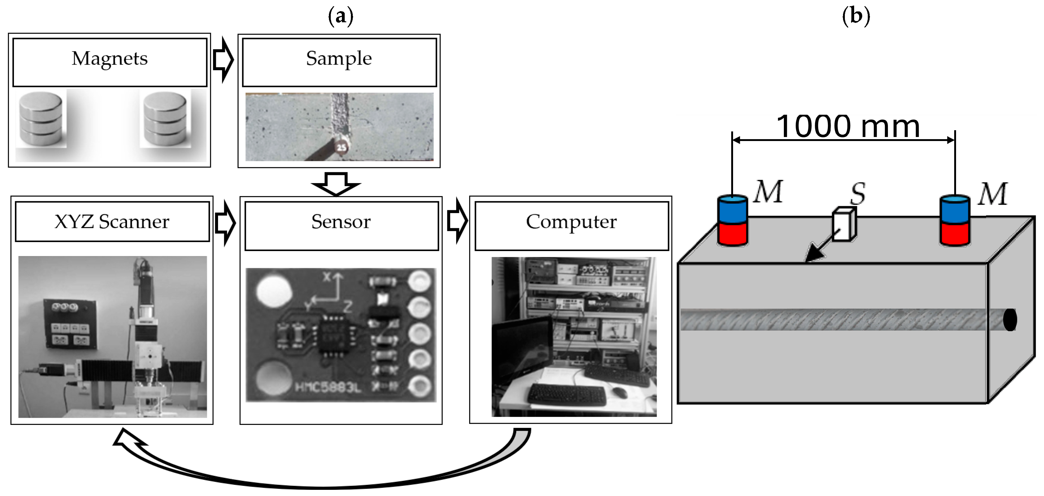
• The excitation system consists of two neodymium magnets. These strong magnets effectively magnetize the reinforcing bars, eventually producing a significantly stronger signal than the EC method.
• The magnets are oriented with the same poles toward the sample (same-pole magnetization—SPM). This configuration allows for a much higher signal-to-noise ratio than the standard opposite-pole magnetization (OPM) [71] and facilitates the construction of area transducers [41];
• The high distance between the magnets and the transducer (500 mm) significantly limits direct interaction. In this method, the only adjustable parameters are the strength of the magnets and the distance between them (Figure 12b). This setup also facilitates the development of an area-testing transducer [41];
• The stationary magnets are placed directly above the tested rebar (no movement during measurement). This minimizes the influence of neighbor rebars in the reinforcement grid on measurement results, allowing for effective measurements even at much greater distances than those achievable with EC.

Similarly, like in the case of the EC method, the most typical technology for this method was selected. The AMR sensor (HMC5883L, Honeywell, NJ, USA [70]) satisfies the fundamental requirements (Figure 1) and possesses several advantageous features. The element enables measurement of the spatial components of magnetic induction (B_x, B_y, and B_z) and can detect negative values, which facilitates polarization recognition. Furthermore, it reduces the risk of damage in cases where the measurement range is exceeded, thereby enhancing system reliability. The design of the measurement system is simplified due to the sensor’s integration capabilities, contributing to its cost-effectiveness. Moreover, the AMR sensor exhibits high sensitivity and resolution, making it well-suited for precise measurements.

3. Results

3.1. Initial Measurements

3.1.1. Measurements in Eddy Current and Magnetic Experiments

The results obtained from eddy current (EC) measurements are characterized by magnitude and phase shift (which can be easily converted to complex numbers—imaginary (Im) and real (Re) components). Figure 14 presents an example of EC measurement.

The phase shift value only yields information about the rebar’s position. Subsequent analyses are, therefore, focused on the magnitude.

AMR sensors allow for the analysis of all three spatial components of magnetic induction (B). Figure 15 illustrates sample waveforms.

Considering the results’ symmetry and the measurements’ time-consuming nature in both methods, the measurement range is limited. Only half of the waveform (to the rebar or from the rebar) is analyzed.

The results shown in Figure 13 and Figure 15 reveal that when the excitation moves along with the sensor (as in the EC method), the resulting waveform exhibits more dynamic variations compared to the magnetic method, where the excitation remains stationary. This characteristic is advantageous for assessing dense reinforced meshes. Rebars are typically spaced 10, 15, or 20 cm apart in a standard reinforcing mesh. When the distance between rebars is only 10 cm, there is a significant risk that the nearby bar will affect the shape factors related to lower amplitude percentages, such as d₁₀ and d₂₀. The smaller transducer can be utilized in such situations to solve this problem. However, this change will negatively impact the effective range of the method. Experiments show that even transducer T25 is ineffective at evaluating rebars placed at distances higher than 60 mm from the transducer. Small transducers like T5 become ineffective if h exceeds 40 mm.

The magnetic method utilizes a distinct approach from the EC method. A magnetized rebar can be detected from a considerable distance. However, the magnetic field of the magnetized rebar is significantly stronger (up to ten times [44]) than that of unmagnetized rebars, which reduces the influence of other elements in the reinforcing mesh. To further diminish the impact of neighboring rebars, all rebars in the measurement area can be demagnetized (remove residual magnetization) before testing with a strong electromagnet powered by alternating current. This procedure effectively reduces their influence and improves the effectiveness of the method.

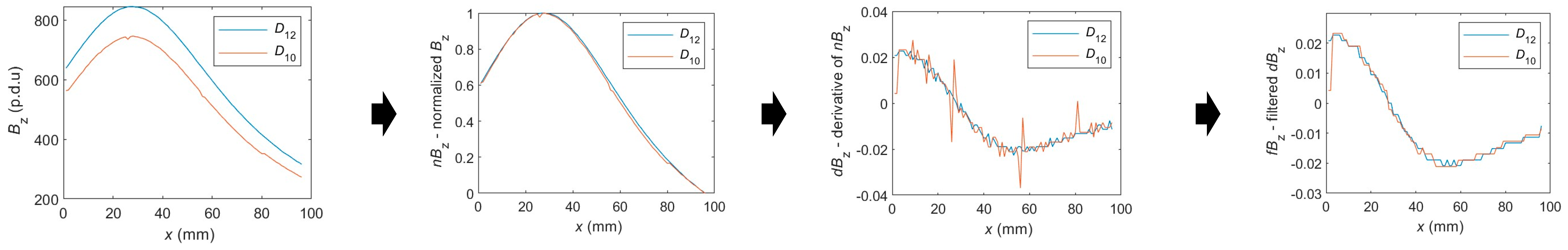
3.1.2. Features Extraction from Measurement Waveforms

Following the preliminary analysis of the statistics and charts (e.g., Figure 13 and Figure 15), the following conclusions regarding the features were drawn:

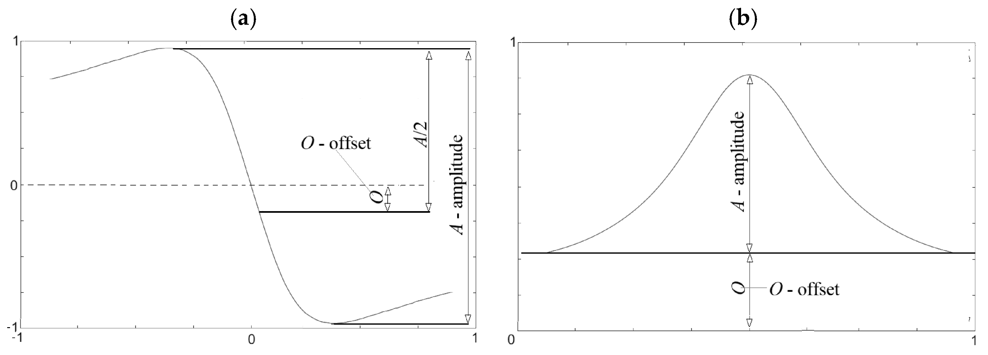
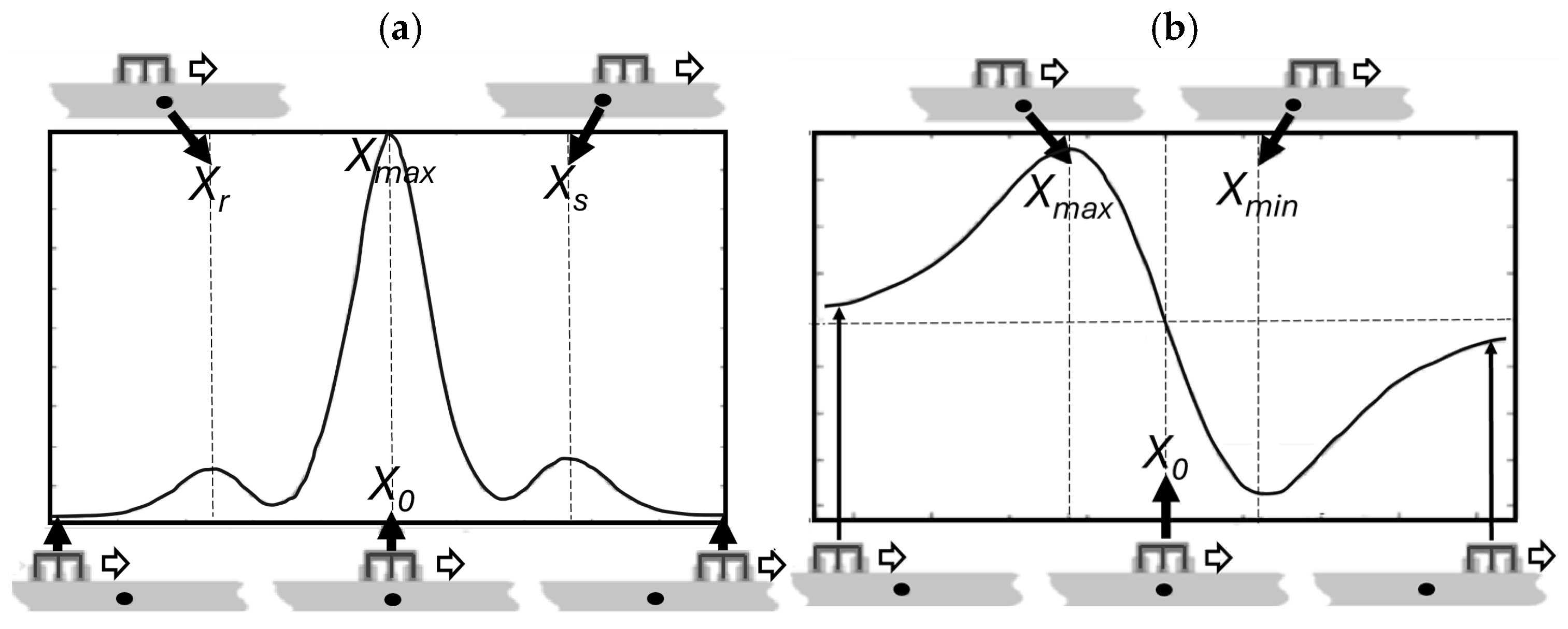
• Unlike the EC waveforms, the magnetic measurements display an offset that can be utilized as a distinct attribute;
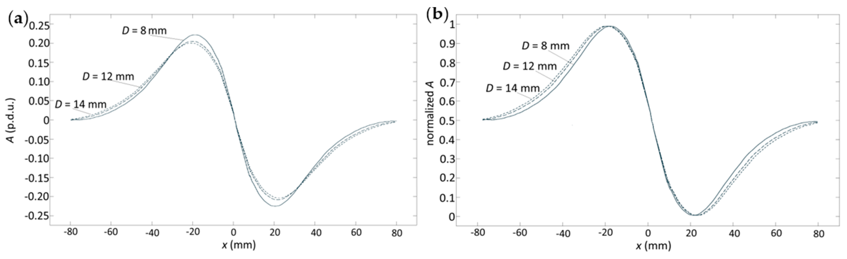
• Attributes obtained from the B_x component (MFL method) and magnitude (EC method) can be determined using the same approach (presented in Figure 5);
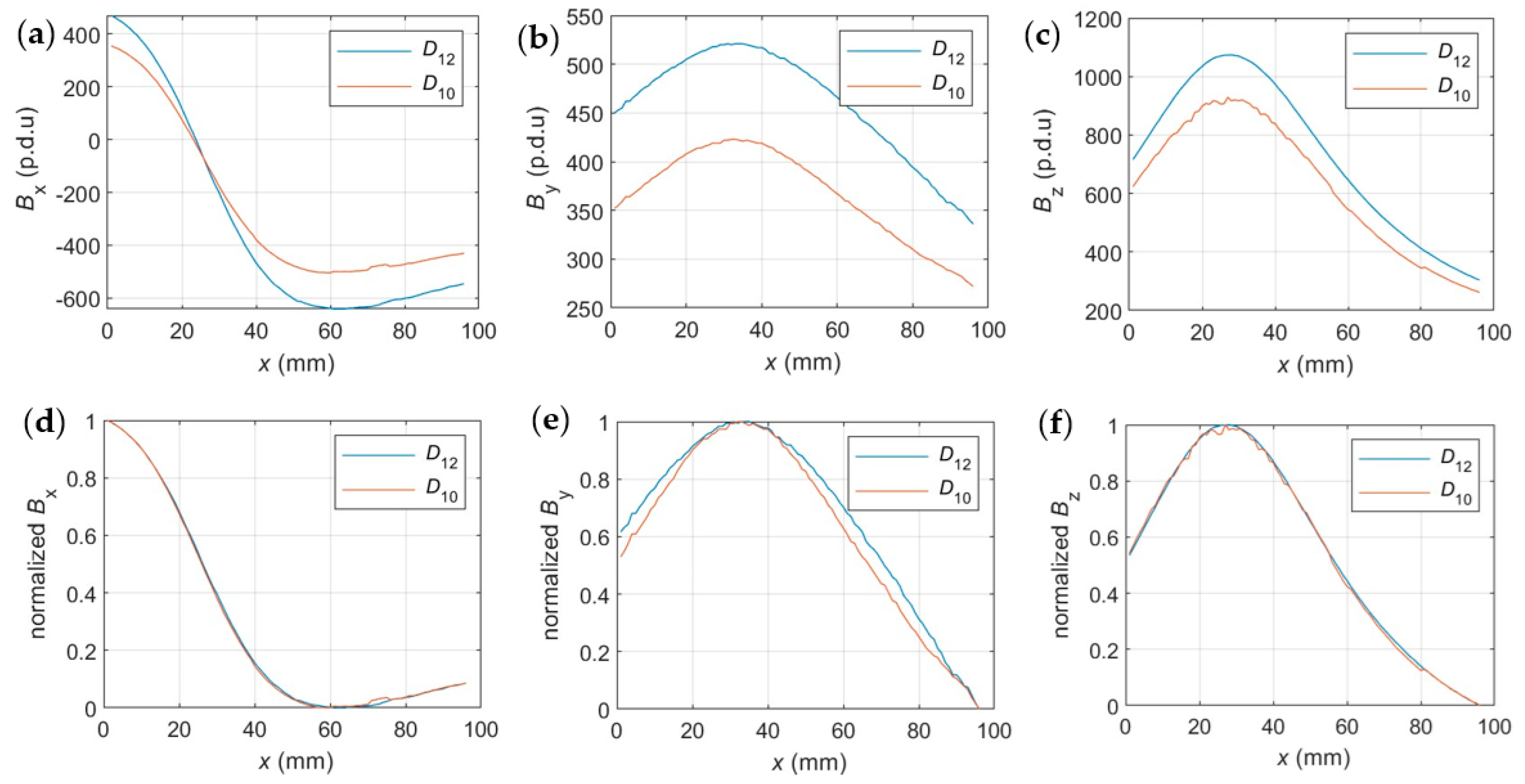
• For spatial components B_y and B_z, the equal intervals in the domain of amplitude method were employed to extract attributes.

Minimizing the number of shape attributes while improving their effectiveness is complex. The research on these features is centered around identifying the diameter of reinforcing bars (the most challenging task in this study). Preliminary tests have indicated that the attributes (such as d₃₀) are ineffective at identifying the rebar diameter. The problem comes from too small differences in the shapes of waveforms obtained from rebars with only a 2 mm diameter variation (basic association rules confirm this observation—see

Table 2. Basic association rules for evaluating variations in rebar diameter using shape attributes ΔD = 2 mm ↑.

Feature	EC method—magnitude waveform					MFL method—Bx waveform
	${\mathit{d}}_{10}$	${\mathit{d}}_{30}$	${\mathit{d}}_{50}$	${\mathit{d}}_{70}$	${\mathit{d}}_{90}$	${\mathit{d}}_{10}$	${\mathit{d}}_{30}$	${\mathit{d}}_{50}$	${\mathit{d}}_{70}$	${\mathit{d}}_{90}$
Change	↑	↑	↑	↑	↑	↑	↑	↑	↑	↑
Confidence (%)	75	85	80	72	60	52	65	71	63	52
Support (%)	33	33	33	33	33	14	14	14	14	14
Feature	MFL method—By waveform					MFL method—Bz waveform
	${\mathit{d}}_{10}$	${\mathit{d}}_{30}$	${\mathit{d}}_{50}$	${\mathit{d}}_{70}$	${\mathit{d}}_{90}$	${\mathit{d}}_{10}$	${\mathit{d}}_{30}$	${\mathit{d}}_{50}$	${\mathit{d}}_{70}$	${\mathit{d}}_{90}$
Change	↑	↑	↑	↑	↑	↑	↑	↑	↑	↑
Confidence (%)	63	74	75	69	55	53	67	69	62	54
Support (%)	14	14	14	14	14	14	14	14	14	14

).

Experiments are conducted on four pairs of rebars (including additional measurements) for the EC method, whereas only one pair is tested for the magnetic method. Statistical analyses are performed for four concrete cover thicknesses, ranging from 20 to 50 mm in 10 mm increments. The T25 transducer was used in the EC method experiments.

The association rules presented in Table 2 are relatively weak. The spatial resolution of the EC method is significantly better than that of the magnetic method, leading to much higher confidence values. However, even with the biggest transducer, the EC method performs poorly with high concrete cover thicknesses (h). Consequently, the study area was restricted to a range of h from 10 to 50 mm for a preliminary test (the typical concrete cover thickness is between 20 and 50 mm). Shape attributes are derived from normalized waveforms. Therefore, those related to high amplitude values (such as d₇₀ and d₉₀) have low confidence due to the decreasing distance between measurements as they approached the peak (value 1). Additionally, attributes corresponding to low amplitude values (e.g., d₁₀) yielded worse results because of the low signal-to-noise ratio (SNR) associated with these measurements (noise has a more pronounced effect when the signal is weak). The influence of the concrete cover thickness on the shape attributes is shown in Figure 16.

The shape attributes show a linear correlation with the thickness of the concrete cover (h). The results of the T25 transducer demonstrate the lowest standard deviation around h = 30 mm. Below h = 20 mm, a significant unwanted influence of the excitation coils on the rebar is observed. When for h higher than 45 mm, the impact of noise becomes a more critical factor. To improve the usability of shape attributes and reduce their number, all shape attributes from d₃₀ to d₇₀ (which demonstrated the lowest standard deviation) are averaged together. This aggregation minimizes the influence of noise and highlights the differences between waveforms. The resulting feature is called d_s. Statistically, d_x is the most effective shape attribute. Figure 17 illustrates the relationships between values of d_s and d_x and the thickness of the concrete cover.

Attribute d_x can be easily extracted from the EC magnitude waveform (when using a differential transducer) and the spatial component of magnetic induction B_x (magnetic method). In the case of B_y and B_z components, the X coordinates of the inflection points of the waveforms are analyzed to determine this parameter. However, calculating the derivative from the waveform significantly amplifies the impact of noise on the attribute value. Therefore, the waveforms are also filtered with a median filter. The whole process is presented in Figure 18.

3.1.3. Transducers

The selection of transducer size is crucial in eddy current (EC) testing. Figure 19 and

Table 3. Linear approximation of measurement results for different transducers; equations of the line and correlation coefficient (r).

	P5	P13	P20	P25
dx	3.67 + 0.38 h	7.56 + 0.33 h	8.30 + 0.32 h	10.12 + 0.32 h
R	96.621%	96.998%	99.555%	99.248%

and

Table 4. Basic statistics for different transducers and concrete cover thickness: average ($\overline{x}$), standard deviation ($\sigma$) and range (R).

	$\mathit{h}\mathbf{=}$ 10 mm			$\mathit{h}\mathbf{=}$ 15 mm			$\mathit{h}\mathbf{=}$ 20 mm			$\mathit{h}\mathbf{=}$ 25 mm			$\mathit{h}\mathbf{=}$ 30 mm
	$\overline{\mathit{x}}$	$\mathit{\sigma }$	R	$\overline{\mathit{x}}$	$\mathit{\sigma }$	R	$\overline{\mathit{x}}$	$\mathit{\sigma }$	R	$\overline{\mathit{x}}$	$\mathit{\sigma }$	R	$\overline{\mathit{x}}$	$\mathit{\sigma }$	R
P5	8.0	0.32	0.6	9.4	0.25	0.6	11.2	0.31	0.6	13.0	0.29	0.6	15.0	0	0
P13	11.0	0.32	0.6	12.5	0	0	14.0	0.32	0.6	16.2	0.92	1.8	16.5	0.85	2.1
P20	11.7	0.18	0.6	13.4	0	0	14.6	0	0	16.2	0.32	0.6	17.6	0.18	0.6
P25	13.4	0.33	0.6	15.3	0.33	0.6	16.7	0.42	1.2	18.1	0.42	1.2	19.1	0.23	0.6
	$\mathit{h}=$ 35 mm			$\mathit{h}\mathbf{=}$ 40 mm			$\mathit{h}=$ 45 mm			$\mathit{h}\mathbf{=}$ 50 mm			$\mathit{h}\mathbf{=}$ 55 mm
	$\overline{\mathit{x}}$	$\mathit{\sigma }$	R	$\overline{\mathit{x}}$	$\mathit{\sigma }$	R	$\overline{\mathit{x}}$	$\mathit{\sigma }$	R	$\overline{\mathit{x}}$	$\mathit{\sigma }$	R	$\overline{\mathit{x}}$	$\mathit{\sigma }$	R
P5	16.3	0.55	1.2	18.4	0.92	3.1	20.4	1.39	4.9	21.4	1.23	2.4	26.2	3.50	8.5
P13	19.3	0.92	1.8	20.2	0.49	1.2	21.7	0.25	0.6	24.5	2.20	4.9	25.6	2.32	6.1
P20	19.2	0.32	0.6	20.7	0.27	1.2	22.7	0.37	1.2	24.3	0.81	2.4	26.3	0.57	1.8
P25	21.0	0	0	22.6	0.33	0.6	24.5	0.46	1.2	26.0	1.25	3.7	28.1	0.48	1.2

illustrate a comparison of four different transducers.

Across the entire spectrum of tested concrete cover thicknesses (h), larger transducers demonstrate greater usability, as evidenced by a higher correlation coefficient. Furthermore, the transducer’s quality (especially the coil’s winding) significantly impacts non-destructive testing (NDT) results. It was noted that despite being larger, the T25 transducer exhibited a lower correlation coefficient than the T20. This fact is also confirmed by Table 4, which provides statistics, including the mean, standard deviation, and range for different values of h and various transducers.

The statistics presented in Table 4 confirm that smaller transducers generally gave better results with thin concrete cover; larger transducers tend to perform better at higher h and across a broader range. However, Table 4 also highlights the impact of the transducer’s quality on results. Despite its relatively large size, the T20 performed exceptionally well across nearly all concrete cover thicknesses.

3.2. Parameter Identification

This paper emphasizes the distinctions and similarities between eddy current (EC) and magnetic flux leakage (MFL) methods rather than the identification process itself. The examples provided primarily serve to compare the two methods. Consequently, the identification problem has been significantly condensed and simplified. A more comprehensive study on the identification can be found in the previous work [44].

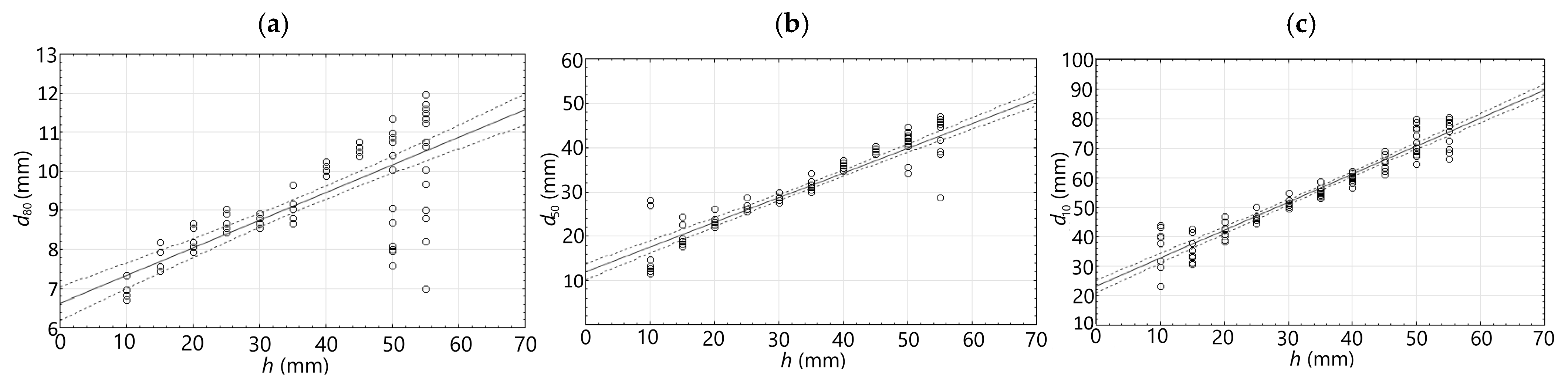
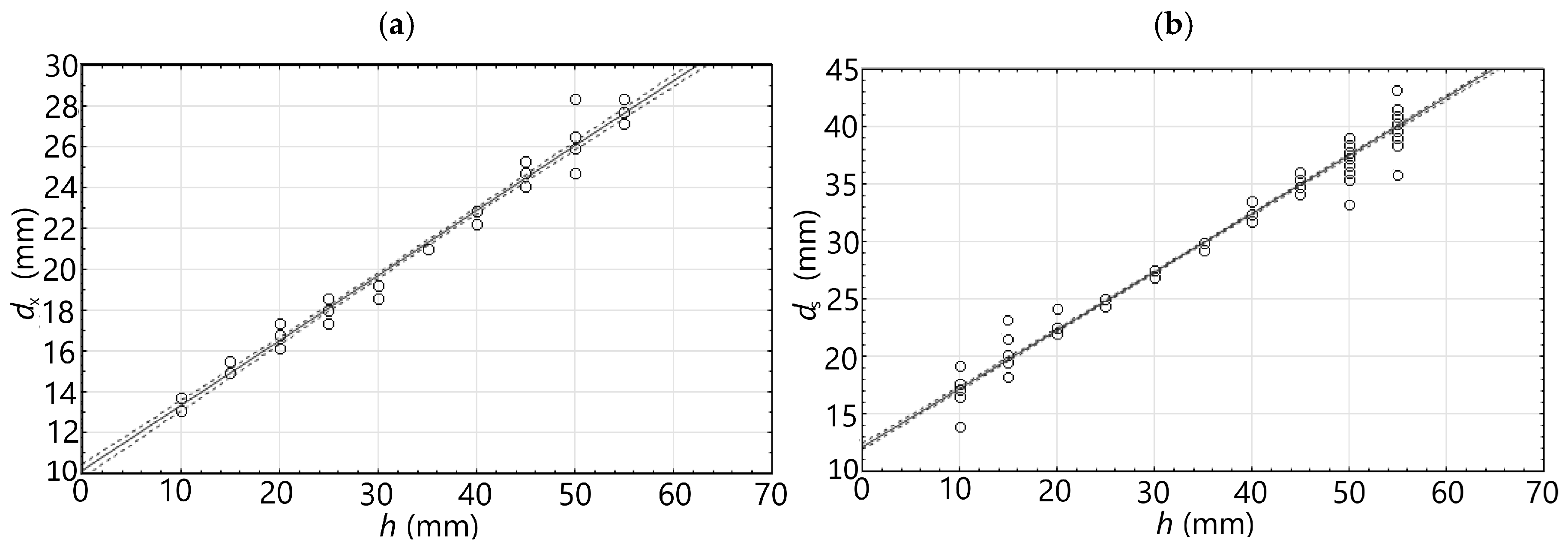
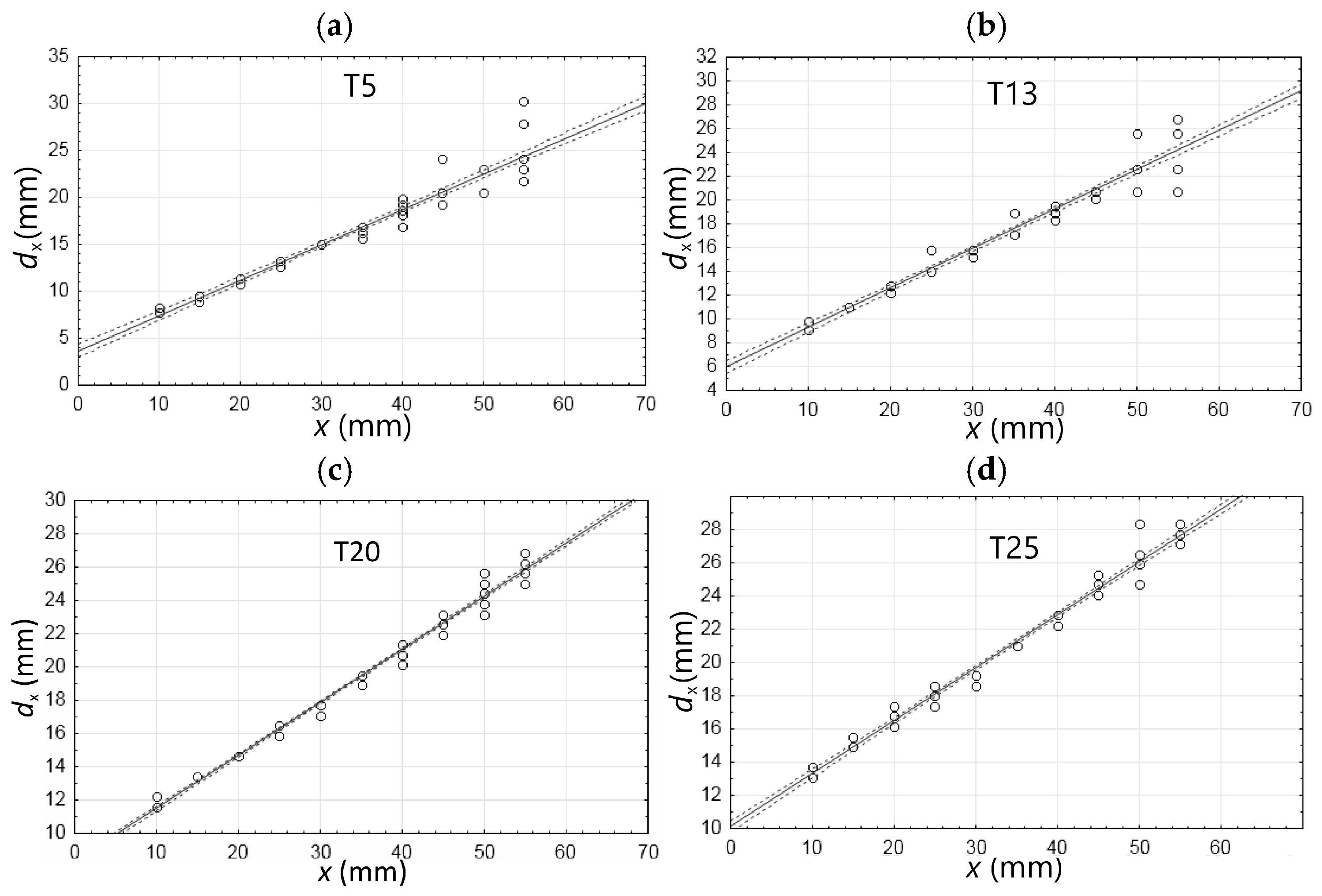
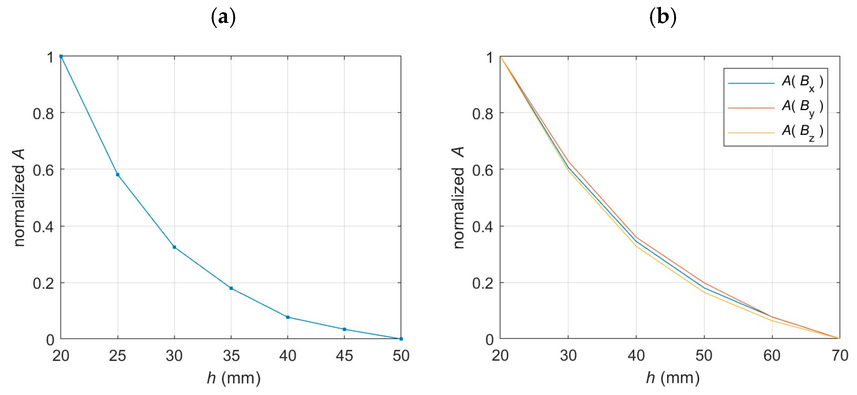
3.2.1. Concrete Cover Thickness

The thickness of the concrete cover (h) is a continuous variable that influences almost all attributes, including amplitude (A), offset (O), and shape attributes (d_x and d_s). The regression and statistical analysis of the h parameter are presented in [44]. Figure 20 illustrates the effect of concrete cover thickness on the measurement waveforms for the eddy current method.

As a preliminary step in this research, association rules have been extracted. These rules provide a deeper insight into the relationships between structural characteristics and waveform features. The fundamental association rules are listed in

Table 5. Basic association rules for assessing changes in rebar diameter based on shape attributes (Δh = 10 mm ↑).

Feature	EC—magnitude						MFL—BX waveform
	A		${\mathit{d}}_{\mathit{x}}$		${\mathit{d}}_{\mathit{s}}$		A	O	${\mathit{d}}_{\mathit{x}}$	${\mathit{d}}_{\mathit{s}}$
Change	↓		↑		↑		↓	-	↑	↑
Confidence (%)	100		95		93		100	100	100	98
Support (%)	50		50		50		57	57	57	57
Feature	MFL—BY waveform						MFL—BZ waveform
	A	O		${\mathit{d}}_{\mathit{x}}$		${\mathit{d}}_{\mathit{s}}$	A	O	${\mathit{d}}_{\mathit{x}}$	${\mathit{d}}_{\mathit{s}}$
Change	↓	↓		↑		↑	↓	↑	↑	↑
Confidence (%)	100	100		98		100	100	56	94	99
Support (%)	57	57		57		57	57	57	57	57

.

In the next step, the curves representing attribute values as a function of h are created to determine the optimal set of attributes. Subsequently, the cross-correlation between these curves is assessed. If the correlation value is high and the standard deviations of the individual parameters are comparable, the attributes are combined to minimize noise interference. On the other hand, any attribute with a significantly higher standard deviation is excluded from the attribute set. This method parallels techniques used in rough set theory.

The investigations (EC method) show a strong correlation between d_x and d_s shape attributes (Figure 17). To mitigate the influence of noise, these attributes are averaged, creating a new shape feature. Before aggregation, the attribute d_x is multiplied by 1.5 to align its values more closely with those of the d_s attribute. Subsequently, the significance of the attributes is assessed first using the InfoGain filter and then through wrappers with the Naive Bayes (NB) classifier. Both attributes (amplitude and the shape attribute d_h) are determined to be significant. The Decision Tree C4.5 algorithm is employed for the final tests. The research in [44] demonstrates the algorithm’s effectiveness at identifying reinforced concrete (RC) structure parameters.

Table 6. Correctness of the concrete cover identification—eddy current method, step of 10 mm.

h (mm)	20	30	40	50	60	70
Correctness of the identification (%)	100	100	100	100	98	95

shows the classification accuracy across different cover thicknesses.

The high identification accuracy is attributed to a substantial step size of 10 mm.

Table 7. Correctness of the concrete cover identification—eddy current method, step of 5 mm.

h (mm)	10	15	20	25	30	35
Correctness of the identification (%)	97	100	99	100	100	100
h (mm)	40	45	50	55	60	70
Correctness of the identification (%)	99	96	95	92	86	93

illustrates results obtained with a smaller step size of 5 mm.

Figure 21 presents the amplitude as a function of h.

The studies conducted on the magnetic method showed a strong correlation among the curves representing the amplitudes of all spatial components as a function of h. These functions closely resemble the corresponding curve obtained from the eddy current tests, although the latter exhibited more dynamic variations. Due to the high correlations observed, the three amplitude features are combined to form a new attribute.

A strong correlation is also noted among the shape attributes (MFL method). The optimal model identified using wrappers included the attribute d_x(B_x). Other shape attributes exhibit a high correlation with it. Among these, the attributes d_x(B_y) and d_x(B_z), derived from the inflection point (Figure 18), displayed the highest standard deviation. Attributes such as O(B_y) and O(B_z) could also be incorporated into the model; however, it is impossible to ascertain which model is superior, as all demonstrate 100% efficiency, as indicated in

Table 8. Correctness of the concrete cover identification—magnetic method, step of 10 mm.

h (mm)	20	30	40	50	60	70
Correctness of the identification (%)	100	100	100	100	100	100

.

The magnetic method is more effective at identifying concrete cover thickness, particularly for higher concrete cover thicknesses. The constructed models and the relationships between attributes are similar. However, the magnetic method allows for the inclusion of offset attributes in the model, which are not available in the eddy current method.

3.2.2. Rebar Diameter

The diameter (D) of the rebar can be regarded as a discrete parameter that affects almost all attributes.

Table 9. Basic association rules for assessing changes in rebar diameter (ΔD = 2 mm ↑).

Feature	EC—magnitude						MFL—BX waveform
	A		${\mathit{d}}_{\mathit{x}}$		${\mathit{d}}_{\mathit{s}}$		A	O	${\mathit{d}}_{\mathit{x}}$	${\mathit{d}}_{\mathit{s}}$
Change	↓		↑		↑		↑	-	↑	↑
Confidence (%)	69		83		90		88	92	84	61
Support (%)	33		33		33		57	57	57	57
Feature	MFL—BY waveform						MFL—BZ waveform
	A	O		${\mathit{d}}_{\mathit{x}}$		${\mathit{d}}_{\mathit{s}}$	A	O	${\mathit{d}}_{\mathit{x}}$	${\mathit{d}}_{\mathit{s}}$
Change	↑	↑		-		↑	↑	↑	-	↑
Confidence (%)	83	99		58		100	90	86	74	83
Support (%)	57	57		57		57	57	57	57	57

presents the basic association rules.

The weak association rules presented in Table 9 indicate that identifying this parameter is difficult. A change in the rebar diameter by 2 mm affects all attributes except the offset B_x. In the case of the eddy current (EC) method, the confidence parameter indicates that the identification will probably be based on the d_s feature. In contrast, in the case of the magnetic flux leakage (MFL) method, the offset parameters (not present in the EC method) and some amplitudes will play a significant role in the identification model (in addition to the ds parameters). The changes in d_x are small. Therefore, this parameter may not be useful, especially for larger cover thicknesses, where noise becomes more important.

Figure 22 and Figure 23 illustrate example results obtained for samples with varying rebar diameters. The results in Figure 22 support the conclusions drawn from the basic association rules presented in Table 5, indicating that the diameter affects nearly all attributes, albeit with minimal variations. The changes in the d_s parameter are both significant and linear as a function of D. At the same time, changes in the d_x parameter are also linear with respect to D, but they are relatively small. A more thorough analysis indicates that a 2 mm change in diameter has effects comparable to a 2 mm change in concrete cover thickness.

Similar to the concrete cover thickness, further analyses were conducted. The optimal model for the EC method included all three attributes. For the MFL method, the model utilized the aggregated amplitude, d_s(B_y), and O(B_y). Including the aggregated offset could also be considered, as it slightly enhances the results for larger cover thicknesses, although it negatively impacts performance for smaller thicknesses. The classification results are illustrated in Figure 24.

The investigation into the diameter of reinforcing bars confirmed that the magnetic MFL method yields superior results across a broad measurement range. Conversely, the eddy current method performed slightly better than MFL when the transducer operated within its optimal measurement range. This advantage can be attributed to the higher spatial resolution associated with this type of transducer.

A significant drawback of the eddy current method is that an increase in rebar diameter produces changes that closely resemble those resulting from an increase in concrete cover thickness. This issue is not present with the MFL method.

3.2.3. Reinforced Steel Class

The steel class is a discrete parameter that affects only amplitude and offset.

Table 10. Basic association rules for assessing changes in steel class (class ↑).

Feature	EC—magnitude						MFL—BX waveform
	A		${\mathit{d}}_{\mathit{x}}$		${\mathit{d}}_{\mathit{s}}$		A	O	${\mathit{d}}_{\mathit{x}}$	${\mathit{d}}_{\mathit{s}}$
Change	↓		-		-		↑	↑	-	-
Confidence (%)	69		83		90		94	92	86	89
Support (%)	17		17		17		29	29	29	29
Feature	MFL—BY waveform						MFL—BZ waveform
	A	O		${\mathit{d}}_{\mathit{x}}$		${\mathit{d}}_{\mathit{s}}$	A	O	${\mathit{d}}_{\mathit{x}}$	${\mathit{d}}_{\mathit{s}}$
Change	↓	↓		-		-	↑	↑	-	-
Confidence (%)	52	57		78		87	99	100	85	91
Support (%)	29	29		29		29	29	29	29	29

presents the basic association rules.

Table 10 illustrates that changes in rebar class do not influence the shape attributes for either method. The weak association rules obtained for the By component indicate that B_y attributes should be excluded from the model. Figure 25 and Figure 26 illustrate example results obtained for samples with varying rebar classes.

Figure 25 and Figure 26 corroborate the findings presented in Table 6. The identification model for the EC method solely incorporates the A feature. In contrast, the optimal attribute set for the MFL method includes both the aggregated amplitude and offset, while features derived from B_y are excluded.

The results of steel class identification are presented in Figure 27.

The investigation into steel class confirmed that the magnetic MFL method performs better across a wide measurement range. However, the eddy current method slightly outperforms MFL when the transducer is within its optimal range. Moreover, changes in rebar class affect the EC and MFL methods differently, with stronger effects observed in the EC method.

4. Conclusions

According to the literature review, the eddy current method (EC) and the magnetic MFL methods are irreplaceable for assessing objects a few centimeters apart (like rebar in reinforced concrete RC structures). Other methods operating in this range (radiography or ultrasounds) have severe limitations in testing RC structures. The EC and MFL methods share similar principles and can be utilized for comparable tasks. A vital advantage of the magnetic method is its ability to employ strong excitation through permanent magnets, resulting in a significantly greater effective range. Experiments show that the MFL method enables effective identification in the typical range of concrete cover thicknesses (or higher). The effective range of the EC method depends on transducer size, used excitation frequency, quality of the transducer, and many other factors. However, experiments prove that the effective range of such transducers is usually limited to a few centimeters. (Figure 24 and Figure 27). Therefore, the MFL method is preferable for testing RC structures.

On the other hand, the EC method offers significantly better spatial resolution, making it effective for detecting small changes, such as a 2 mm diameter variation. However, it is challenging to construct an EC transducer capable of covering the entire typical range of concrete cover thicknesses within its optimal range. The MFL method offers better average identification in the whole range of measurements (depending on the EC transducer size and tested parameter, this difference can exceed 10%). However, if the EC transducer works in the optimal range (usually low concrete cover thickness), the obtained results can be significantly better than those of MFL (usually 3–10%). The EC method may be more effective than MFL when the concrete cover thickness is low, and variations in the value of the h parameter are low. Employing a set of EC transducers of varying sizes would be beneficial for achieving comprehensive identification.

The higher effectiveness of the MFL method also comes from other facts. The magnetic method can utilize offsets for identification, which was quite beneficial during the research. In the case of the EC method, the offset is always equal to 0. Moreover, magnetic systems and transducers are generally more straightforward and cost-effective. They also allow for area measurements.

In conclusion, the research suggests that the magnetic MFL method is more effective for identifying typical reinforced concrete structures.

Small eddy current (EC) transducers, like the T5, demonstrate superior performance at low concrete cover thicknesses, achieving up to 5–10% better identification than larger transducers, such as the T25. Conversely, larger transducers tend to perform better (also by 5–10%) when the concrete cover thickness is greater. When averaging typical ranges of concrete cover thicknesses, larger transducers generally perform better than their smaller counterparts.

References

1. PN-B-03264:2002; Concrete, Reinforced Concrete and Prestressed Structures. Static Calculations and Design. PKN: Warsaw, Poland, 2002.
2. Smith, D.G.E.; Brown, R.H. Reinforced Concrete Design, 10th ed.; Mercury Learning and Information: Herndon, VA, USA, 2021; ISBN 9781683929079. [Google Scholar]
3. Mosley, B.; Hulse, R.; Bungey, J. Reinforced Concrete Design: To Eurocode 2; Palgrave Macmillan: London, UK, 2012; ISBN 9780230302853. [Google Scholar]
4. Drobiec, Ł.; Jasiński, R.; Piekarczyk, A. Diagnostyka Konstrukcji Żelbetowych; PWN: Warszawa, Poland, 2010; Volume 1, ISBN 978-83-01-16103-3. [Google Scholar]
5. Zybura, A.; Jaśniok, A.; Jaśniok, T. Diagnostyka Konstrukcji Żelbetowych; PWN: Warszawa, Poland, 2021; Volume 2, ISBN 978-83-01-16698-4. [Google Scholar]
6. Frankowski, P.K.; Chady, T.; Zieliński, A. Magnetic force induced vibration evaluation (M5) method for frequency analysis of rebar-debonding in reinforced concrete. Measurement 2021, 182, 109655. [Google Scholar] [CrossRef]
7. Masoumi, F.; Akgül, F.; Mehrabzadeh, A. Condition Assessment of Reinforced Concrete Bridges by Combined Nondestructive Test Techniques. Int. J. Eng. Technol. 2013, 5, 708–711. [Google Scholar] [CrossRef]
8. Verma, S.K.; Bhadauria, S.S.; Akhtar, S. Review of Nondestructive testing methods for condition monitoring of concrete structures. J. Constr. Eng. 2013, 2013, 834572. [Google Scholar] [CrossRef]
9. Bui, H.; Delattre, F.; Levacher, D. Experimental Methods to Evaluate the Carbonation Degree in Concrete—State of the Art Review. Appl. Sci. 2023, 13, 2533. [Google Scholar] [CrossRef]
10. Wiwatrojanagul, P.; Sahamitmongkol, R.; Tangtermsirikul, S.; Khamsemanan, N. A new method to determine locations of rebars and estimate cover thickness of RC structures using GPR data. Constr. Build. Mater. 2017, 140, 257–273. [Google Scholar] [CrossRef]
11. Dinh, K.; Gucunski, N.; Duong, T.H. An algorithm for automatic localization and detection of rebars from GPR data of concrete bridge decks. Autom. Constr. 2018, 89, 292–298. [Google Scholar] [CrossRef]
12. Mechbal, Z.; Khamlichi, A. Determination of concrete rebars characteristics by enhanced post-processing of GPR scan raw data. NDT E Int. 2017, 89, 30–39. [Google Scholar] [CrossRef]
13. Dinh, K.; Gucunski, N.; Duong, T.H. Migration-based automated rebar picking for condition assessment of concrete bridge decks with ground penetrating radar. NDT E Int. 2018, 98, 45–54. [Google Scholar] [CrossRef]
14. Dong, B.; Shi, G.; Dong, P.; Ding, W.; Teng, X.; Qin, S.; Liu, Y.; Xing, F.; Hong, S. Visualized tracing of rebar corrosion evolution in concrete with x-ray micro-computed tomography method. Cem. Concr. Compos. 2018, 92, 102–109. [Google Scholar] [CrossRef]
15. Sadowski, L. Methodology for Assessing the Probability of Corrosion in Concrete Structures on the Basis of Half-Cell Potential and Concrete Resistivity Measurements. Sci. World J. 2013, 2013, 714501. [Google Scholar] [CrossRef]
16. Gu, P.; Beaudoin, J.J. Obtaining Effective Half-Cell Potential Measurements in Reinforced Concrete Structures; Construction Technology Updates; National Research Council of Canada: Ottawa, ON, Canada, 1998; ISSN 1206-1220.
17. Nguyen, A.; Klysz, G.; Deby, F.; Balayssac, J. Assessment of the electrochemical state of steel reinforcement in water saturated concrete by resistivity measurement. Constr. Build. Mater. 2018, 171, 455–466. [Google Scholar] [CrossRef]
18. Lim, Y.-C.; Noguchi, T.; Cho, C.-G. A quantitative analysis of the geometric effects of reinforcement in concrete resistivity measurement above reinforcement. Constr. Build. Mater. 2015, 83, 189–193. [Google Scholar] [CrossRef]
19. Lim, Y.-C.; Noguchi, T.; Cho, C.-G. Mathematical modeling for quantitative estimation of geometric effects of nearby rebar in electrical resistivity measurement. Cem. Concr. Compos. 2018, 90, 82–88. [Google Scholar] [CrossRef]
20. International Atomic Energy Agency. Training Course SERIES No. 17: Guidebook on Non-Destructive Testing of Concrete Structures, Vienna: International Atomic Energy Agency. 2002. Available online: https://www-pub.iaea.org/MTCD/Publications/PDF/TCS-17_web.pdf (accessed on 27 October 2024).
21. Ikumapayi, C.M.; Adeniji, A.A.; Obisesan, A.A.; Odeyemi, O.; Ajayi, J.A. Effects of Carbonation on the Properties of Concrete. Sci. Rev. 2019, 5, 205–214. [Google Scholar] [CrossRef]
22. Szymanik, B.; Chady, T.; Frankowski, P.K. Inspection of reinforcement concrete structures with active infrared thermography. In 43rd Annual Review of Progress in Quantitative Non-Destructive Evaluation; AIP: Melville, NY, USA, 2017; Volume 36, ISBN 9780735414747. [Google Scholar] [CrossRef]
23. Keo, S.A.; Szymanik, B.; Le Roy, C.; Brachelet, F.; Defer, D. Defect Detection in CFRP Concrete Reinforcement Using the Microwave Infrared Thermography (MIRT) Method—A Numerical Modeling and Experimental Approach. Appl. Sci. 2023, 13, 8393. [Google Scholar] [CrossRef]
24. Szymanik, B.; Keo, S.A.; Brachelet, F.; Defer, D. Investigation of Carbon Fiber Reinforced Polymer Concrete Reinforcement Ageing Using Microwave Infrared Thermography Method. Appl. Sci. 2024, 14, 4331. [Google Scholar] [CrossRef]
25. Ohtsu, M.; Isoda, T.; Tomoda, Y. Acoustic Emission Techniques Standardized for Concrete Structures. Acoustic Emission Group. 2007. Available online: https://www.ndt.net/article/jae/papers/25-021.pdf (accessed on 27 October 2024).
26. Oshita, H. 9—Quantitative estimation of rebar corrosion in reinforced concrete by thermography. In Acoustic Emission and Related Non-Destructive Evaluation Techniques in the Fracture Mechanics of Concrete; Fundamentals and Applications; Woodhead Publishing Series in Civil and Structural Engineering; Woodhead Publishing: Cambridge, UK, 2015; pp. 177–203. [Google Scholar] [CrossRef]
27. Dixit, M.; Gupta, A.K. A Review of Different Assessment Methods of Corrosion of Steel Reinforcement in Concrete. Iran. J. Sci. Technol. Trans. Civ. Eng. 2022, 46, 735–752. [Google Scholar] [CrossRef]
28. Laureti, S.; Ricci, M.; Mohamed, M.; Senni, L.; Davis, L.; Hutchins, D. Detection of rebars in concrete using advanced ultrasonic pulse compression techniques. Ultrasonics 2018, 85, 31–38. [Google Scholar] [CrossRef]
29. Mayakuntla, P.K.; Ganguli, A.; Smyl, D. Gaussian Mixture Model-Based Classification of Corrosion Severity in Concrete Structures Using Ultrasonic Imaging. J. Nondestruct. Eval. 2023, 42, 28. [Google Scholar] [CrossRef]
30. Mayakuntla, P.K.; Ghosh, D.; Ganguli, A. Nondestructive evaluation of rebar corrosion in concrete structures using ultrasonics and laser-based sensing. Nondestruct. Test. Eval. 2021, 37, 297–314. [Google Scholar] [CrossRef]
31. Ghosh, D.; Kumar, R.; Ganguli, A.; Mukherjee, A. Nondestructive Evaluation of Rebar Corrosion-Induced Damage in Concrete through Ultrasonic Imaging. J. Mater. Civ. Eng. 2020, 32, 04020294. [Google Scholar] [CrossRef]
32. Gunes, B.; Gunes, O. Vibration-Based Damage Evaluation of a Reinforced Concrete Frame Subjected to Cyclic Pushover Testing. Shock. Vib. 2021, 2021, 6666702. [Google Scholar] [CrossRef]
33. Caballol, D.; Raposo, P.; Gil-Carrillo, F. Non-destructive testing of concrete layer adhesion by means of vibration measurement. Constr. Build. Mater. 2023, 411, 134548. [Google Scholar] [CrossRef]
34. Szymanik, B.; Frankowski, P.K.; Chady, T.; Chelliah, C.R.A.J. Detection and Inspection of Steel Bars in Reinforced Concrete Structures Using Active Infrared Thermography with Microwave Excitation and Eddy Current Sensors. Sensors 2016, 16, 234. [Google Scholar] [CrossRef] [PubMed]
35. Chady, T.; Frankowski, P. Electromagnetic Evaluation of Reinforced Concrete Structure. In Proceedings of the Review of Progress in Quantitative Non-Destructive Evaluation, Denver, CO, USA, 15–20 July 2012; Volume 32, pp. 1355–1362. [Google Scholar] [CrossRef]
36. Frankowski, P.K. Eddy current method for identification and analysis of reinforcement bars in concrete structures. In Proceedings of the Electrodynamic and Mechatronic Systems, Opole, Poland, 6–8 October 2011; pp. 105–109. [Google Scholar] [CrossRef]
37. Alcantara, N. Identification of steel bars immersed in reinforced concrete based on experimental results of eddy current testing and artificial neural network analysis. Nondestruct. Test. Eval. 2013, 28, 58–71. [Google Scholar] [CrossRef]
38. Xia, Z.; Huang, R.; Chen, Z.; Yu, K.; Zhang, Z.; Salas-Avila, J.R.; Yin, W. Eddy Current Measurement for Planar Structures. Sensors 2022, 22, 8695. [Google Scholar] [CrossRef]
39. Drobiec, Ł.; Jasiński, R.; Mazur, W. Accuracy of Eddy-Current and Radar Methods Used in Reinforcement Detection. Materials 2019, 12, 1168. [Google Scholar] [CrossRef]
40. Frankowski, P.K.; Chady, T. Evaluation of Reinforced Concrete Structures with Magnetic Method and ACO (Amplitude-Correlation-Offset) Decomposition. Materials 2023, 16, 5589. [Google Scholar] [CrossRef]
41. Frankowski, P.K.; Chady, T. Multisensory Spatial Analysis and NDT Active Magnetic Method for Quick Area Testing of Reinforced Concrete Structures. Materials 2023, 16, 7296. [Google Scholar] [CrossRef]
42. Bektaş, Ö.; Kurban, Y.; Özboylan, B. Development of magnetic flux leakage device as a non-destructive method for structural reinforcement detection. Mater. Constr. 2022, 72, e273. [Google Scholar] [CrossRef]
43. Li, V.; Demina, L.; Vlasenko, S. Detecting the Diameter and the Depth of Steel Reinforcing Bar in Concrete Using MFL Method. Int. J. Appl. Sci. Curr. Future Res. Trends 2022, 15, 120–128. [Google Scholar] [CrossRef]
44. Frankowski, P.K.; Majzner, P.; Mąka, M.; Stawicki, T.; Chady, T. Magnetic Non-Destructive Evaluation of Reinforced Concrete Structures—Methodology, System, and Identification Results. Appl. Sci. 2024, 14, 11695. [Google Scholar] [CrossRef]
45. Frankowski, P.K. Corrosion detection and measurement using eddy current method. In Proceedings of the 2018 International Interdisciplinary PhD Workshop (IIPhDW), Swinoujście, Poland, 9–12 May 2018. [Google Scholar] [CrossRef]
46. Eddy, I.; Underhill, P.R.; Morelli, J.; Krause, T.W. Pulsed Eddy Current Response to General Corrosion in Concrete Rebar. J. Nondestruct. Eval. Diagn. Progn. Eng. Syst. 2020, 3, 044501. [Google Scholar] [CrossRef]
47. Alcantara, N.P.; Da Silva, F.M.; Guimarães, M.T.; Pereira, M.D. Corrosion Assessment of Steel Bars Used in Reinforced Concrete Structures by Means of Eddy Current Testing. Sensors 2016, 16, 15. [Google Scholar] [CrossRef] [PubMed]
48. Tsukada, K.; Yoshioka, M.; Kiwa, T.; Hirano, Y. A magnetic flux leakage method using a magnetoresistive sensor for nondestructive evaluation of spot welds. NDT E Int. 2011, 44, 101–105. [Google Scholar] [CrossRef]
49. Rehmat, A.; Sadeghnejad, A.C. Valikhani and others: Magnetic Flux Leakage Method for Detecting Corrosion in Post Tensioned Segmental Concrete Bridges in Presence of Secondary Reinforcement. In Proceedings of the Conference: Transportation Research Board 96th Annual Meeting, Washington, DC, USA, 8–12 January 2017; pp. 8–12. [Google Scholar]
50. Zhang, H.; Liao, L.; Zhao, R.; Zhou, J.; Yang, M.; Zhao, Y. A new judging criterion for corrosion testing of reinforced concrete based on self-magnetic flux leakage. Int. J. Appl. Electromagn. Mech. 2017, 54, 123–130. [Google Scholar] [CrossRef]
51. Shams, S.; Ghorbanpoor, A.; Lin, S.; Azari, H. Nondestructive Testing of Steel Corrosion in Prestressed Concrete Structures using the Magnetic Flux Leakage System. Transp. Res. Rec. J. Transp. Res. Board 2018, 2672, 132–144. [Google Scholar] [CrossRef]
52. Sun, Y.; Liu, S.; Deng, Z.; Tang, R.; Ma, W.; Tian, X.; Kang, Y.; He, L. Magnetic flux leakage structural health monitoring of concrete rebar using an open electromagnetic excitation technique. Struct. Health Monit. 2018, 17, 121–134. [Google Scholar] [CrossRef]
53. Perin, D.; Göktepe, M. Inspection of rebars in concrete blocks. Int. J. Appl. Electromagn. Mech. 2012, 38, 65–78. [Google Scholar] [CrossRef]
54. He, D.; Shiwa, M.; Takaya, S.; Tsuchiya, K. Steel reinforcing bar detection using electromagnetic method. In Proceedings of the 2016 Progress in Electromagnetic Research Symposium (PIERS), Shanghai, China, 8–11 August 2016. [Google Scholar] [CrossRef]
55. Diederich, H.; Vogel, T. Evaluation of Reinforcing Bars Using the Magnetic Flux Leakage Method. J. Infrastruct. Syst. 2017, 23, B4016001. [Google Scholar] [CrossRef]
56. Frankowski, P.K.; Chady, T. Impact of Magnetization on the Evaluation of Reinforced Concrete Structures Using DC Magnetic Methods. Materials 2022, 15, 857. [Google Scholar] [CrossRef] [PubMed]
57. Shearer, C. The CRISP-DM model: The new blueprint for data mining. J. Data Warehous. 2000, 5, 13–22. [Google Scholar]
58. Pawlak, Z. Rough sets. Int. J. Comput. Inf. Sci. 1982, 11, 341–356. [Google Scholar] [CrossRef]
59. Pawlak, Z.; Skowron, A. Rough Set Theory and Its Applications to Data Mining. In Data Mining and Knowledge Discovery; Springer: Berlin/Heidelberg, Germany, 1998; pp. 1–10. [Google Scholar]
60. Agrawal, R.; Mannila, H.; Srikant, R.; Toivonen, H.; Verkamo, A.I. Fast discovery of association rules. In Advances in Knowledge Discovery and Data Mining; Fayyad, U.M., Piatetsky-Shapiro, G., Smyth, P., Uthurusamy, R., Eds.; AAAI Press: Washington, DC, USA, 2021; pp. 307–328. [Google Scholar]
61. Toivonen, H. Apriori Algorithm. In Encyclopedia of Machine Learning and Data Mining; Sammut, C., Webb, G.I., Eds.; Springer: Boston, MA, USA, 2017; p. 60. [Google Scholar] [CrossRef]
62. Tirumalasetty, S.; Aruna, A.; Padmini, A.; Sagaru, D.V.; Tejeswini, A. An Enhanced Apriori with Interestingness of Patterns using cSupport and rSupport. Int. J. Comput. Sci. Mob. Comput. 2021, 10, 20–27. [Google Scholar] [CrossRef]
63. Tirumalasetty, S.; Jadda, A.; Edara, S.R. An Enhanced Apriori Algorithm for Discovering Frequent Patterns with Optimal Number of Scans. arXiv 2015. [Google Scholar] [CrossRef]
64. McCann, D.; Forde, M. Review of NDT methods in the assessment of concrete and masonry structures. NDT E Int. 2001, 34, 71–84. [Google Scholar] [CrossRef]
65. Grochowalski, J.M.; Chady, T. Rapid Identification of Material Defects Based on Pulsed Multifrequency Eddy Current Testing and the k-Nearest Neighbor Method. Materials 2023, 16, 6650. [Google Scholar] [CrossRef]
66. Grochowalski, J.M.; Chady, T. Pulsed Multifrequency Excitation and Spectrogram Eddy Current Testing (PMFES-ECT) for Nondestructive Evaluation of Conducting Materials. Materials 2021, 14, 5311. [Google Scholar] [CrossRef]
67. Chady, T.; Grochowalski, J.M. Eddy Current Transducer with Rotating Permanent Magnets to Test Planar Conducting Plates. Sensors 2019, 19, 1408. [Google Scholar] [CrossRef]
68. Grochowalski, J.M.; Chady, T. Numerical analysis of eddy current transducer with rotating permanent magnets for planar conducting plates testing. In Proceedings of the 2018 International Interdisciplinary PhD Workshop (IIPhDW), Swinoujscie, Poland, 9–12 May 2018. [Google Scholar] [CrossRef]
69. Liu, X.; Zhao, Y.; Sun, M. An Improved Apriori Algorithm Based on an Evolution-Communication Tissue-Like P System with Promoters and Inhibitors. Discret. Dyn. Nat. Soc. 2017, 2017, 6978146. [Google Scholar] [CrossRef]
70. Honeywell. HMC5883L-TR Datasheet. Available online: https://www.allaboutcircuits.com/electronic-components/datasheet/HMC5883L-TR--Honeywell/ (accessed on 29 October 2024).
71. Frankowski, P.K.; Chady, T. A Comparative Analysis of the Magnetization Methods Used in the Magnetic Nondestructive Testing of Reinforced Concrete Structures. Materials 2023, 16, 7020. [Google Scholar] [CrossRef] [PubMed]
Figure 1. Comparison of magnetic sensors based on sensitivity, bandwidth, and size [41]. GMR—giant magnetoresistance; AMR—anisotropic magnetoresistance; TMR—tunnel magnetoresistance; GMI—giant magnetoimpedance; MO—magneto-optical; SQUID—superconducting quantum interference device.
Applsci 14 11965 g001
Figure 2. Methodology for knowledge acquisition from NDT measurement data based on the CRISP-DM model.
Applsci 14 11965 g002
Figure 3. Development evolution of techniques for extracting features from waveforms.
Applsci 14 11965 g003
Figure 4. Attribute extraction process (equal dividing and characteristic points).
Applsci 14 11965 g004
Figure 5. Attribute extraction with equal intervals in the domain of amplitude method.
Applsci 14 11965 g005
Figure 6. The definitions of amplitude and offset: (a) amplitude, (b) offset.
Applsci 14 11965 g006
Figure 7. The algorithm for extracting association rules from NDT data.
Applsci 14 11965 g007
Figure 8. Samples: (a) 3D schematic presentation, (b) cross-section and parameters, (c) parameters.
Applsci 14 11965 g008
Figure 9. Example rebars used during supplementary measurements.
Applsci 14 11965 g009
Figure 10. Block diagram of eddy current system.
Applsci 14 11965 g010
Figure 11. EC transducers used in the experiments: (a) cross-section and description, (b) small T5 transducer, (c) medium T13 transducer, (d) large T20 transducer, (e) largest T25 transducer.
Applsci 14 11965 g011
Figure 12. Waveforms obtained from EC transducers: (a) absolute, (b) differential.
Applsci 14 11965 g012
Figure 13. The magnetic system, (a) block diagram, and (b) elements are arranged on the sample surface. M—magnet, S—sensor.
Applsci 14 11965 g013
Figure 14. Example eddy current measurements: (a) magnitude and phase shift vs. transducer position, (b) real (Re) and imaginary (Im) components vs. transducer position, (c) Im vs. Re.
Applsci 14 11965 g014
Figure 15. Example magnetic measurements with the use of AMR sensor; (a) Bx, (b) By, (c) Bz.
Applsci 14 11965 g015
Figure 16. Impact of concrete cover thickness on shape attributes; (a) d90, (b) d50, (c) d10.
Applsci 14 11965 g016
Figure 17. Impact of concrete cover thickness on high-quality shape attributes; (a) dx, (b) ds.
Applsci 14 11965 g017
Figure 18. Process of dx extraction from By and Bz.
Applsci 14 11965 g018
Figure 19. Linear approximation of measurement results (dx attribute) for different transducers; (a) T5, (b) T13, (c) T20, (d) T25.
Applsci 14 11965 g019
Figure 20. EC transducer—waveforms obtained for different concrete cover thicknesses.
Applsci 14 11965 g020
Figure 21. Amplitude as a function of concrete cover thickness. (a) Eddy current method; (b) magnetic flux leakage method.
Applsci 14 11965 g021
Figure 22. EC—waveforms obtained for different rebar diameters; (a) raw data, (b) normalized data.
Applsci 14 11965 g022
Figure 23. MFL—waveforms obtained for different rebar diameters; (a) Bx, raw data; (b) By, raw data; (c) Bz, raw data; (d) Bx, normalized data; (e) By, normalized data; (f) Bz, normalized data.
Applsci 14 11965 g023
Figure 24. Results of rebar diameter identification derived from both methods across all transducers.
Applsci 14 11965 g024
Figure 25. EC—waveforms obtained for different rebar classes; (a) raw data, (b) normalized data.
Applsci 14 11965 g025
Figure 26. MFL—waveforms obtained for different reinforced steel classes; (a) Bx, raw data; (b) By, raw data; (c) Bz, raw data; (d) Bx, normalized data; (e) By, normalized data; (f) Bz, normalized data.
Applsci 14 11965 g026
Figure 27. Results of steel class identification derived from both methods across all transducers.
Applsci 14 11965 g027