Extending Generalized Explicit Terms and Applying Euler–Bernoulli Beam Theory to Enhance Dynamic Response Prediction in Receptance Coupling Method

Abstract

This paper presents a theoretical framework to enhance the prediction of dynamic responses in complex mechanical systems, such as vehicle structures, by incorporating both translational and rotational degrees of freedom. Traditional receptance coupling methods often neglect rotational effects, leading to significant inaccuracies at higher frequencies. Additionally, approaches that implicitly include full dynamics frequently result in redundancy of generalized coordinates, especially at connection points. To address these limitations, the generalized receptance coupling method using Frequency-Based Substructuring is extended to explicitly account for rotational dynamics resulting in a refined GRCFBS approach. This extension enhances both the understanding and prediction of system responses, which are represented through the receptance matrix or Frequency Response Function. Building on Jetmundsen’s foundational work, the proposed framework introduces a practical, generalized formulation that explicitly incorporates full translational and rotational dynamics at each substructure node. This explicit definition provides deeper insights into system behavior, particularly for complex interactions between substructures under weak and strong coupling scenarios at interface points. The Euler–Bernoulli beam theory is employed to model rotational behavior at critical points, yielding reduced-order and explicit receptance matrices for substructures in the coupling process. The methodology’s accuracy and applicability in capturing resonance and anti-resonance modes are validated through two case studies: the coupling of two flexible subsystems and the integration of flexible and rigid components. Results are benchmarked against numerical finite element analysis, and all limitations and potential improvements are discussed. By directly incorporating rotational dynamics directly, this approach enables more reliable dynamic response predictions under multi-directional loading conditions, particularly for vehicle and machinery system design. The GRCFBS method offers a versatile and reliable tool for dynamic system analysis, with significant potential for vibration analysis over a broad frequency range.

1. Introduction

Dynamic analysis of complex systems, such as vehicles, robots, and machining equipment, has been an area of extensive research, leading to the development of diverse methodologies. Predictive methods like Finite Element Modal Analysis (FEMA) and Dynamic Substructuring (DS) are widely used during the design phase to model and predict dynamic responses, providing insights into natural frequencies, mode shapes, and substructure interactions. On the other hand, diagnostic approaches such as Root Cause Analysis (RCA) and Transfer Path Analysis (TPA) focus on identifying and mitigating vibration issues in operational systems by analyzing energy transmission paths and the sources of vibrational behavior.

Van der Seijs et al. (2016) [1] discussed TPA as a diagnostic tool for vibration and noise issues, classifying it into classical, component-based, and transmissibility-based methods. Similarly, Tuninetti et al. (2021) [2] applied RCA combined with FEMA to diagnose vibration issues using structured cause–effect diagrams. Kong et al. (2024) [3] advanced operational TPA by addressing the challenge of reliable motor controller unit analysis in electric vehicles under real-world conditions. However, their approach lacks a generalized framework for modeling system-wide dynamics.

De Klerk, Rixen, and Voormeeren (2008) [4] provided an extensive framework for DS, a methodology for analyzing complex systems by dividing them into smaller, manageable substructures for independent analysis. DS facilitates modular analysis while maintaining computational efficiency, utilizing techniques such as Component Mode Synthesis (CMS), Impulse-Based Substructuring (IBS), state–space coupling, and Frequency-Based Substructuring (FBS). CMS simplifies large finite element models by retaining key mode shapes (mode truncation), making it suitable for low-frequency applications. State–space coupling complements this by modeling substructures through first-order differential equations and enforcing compatibility at interfaces.

The FBS and IBS approaches are effective for high-frequency applications due to their direct incorporation of receptance or Frequency Response Function (FRF) matrices, preserving damping and complex modes. While IBS leverages impulse response functions (IRFs) for transient or impact loading scenarios in the time domain, FBS synthesizes FRFs in the frequency domain, avoiding mode truncation and ensuring high-frequency dynamics are preserved. Among these, FBS has emerged as a modular approach for analyzing system dynamics by coupling subsystems using experimentally or numerically derived FRFs. Receptance coupling (RC), a subset of FBS, dynamically combines receptance matrices by enforcing compatibility (displacement/moment continuity) and equilibrium (force/moment balance) at subsystem interfaces.

The concept of receptance coupling was first introduced by Bishop and Johnson [5], with subsequent advancements by Gordis, Bielawa, and Flannelly [6] in integrating structural coupling and modification within Finite Element Analysis (FEA). Further advancements were made by Duarte and Ewins [7], who explored translational and rotational parameters for structural coupling analysis using the finite-difference technique. Among the various FBS techniques, the generalized receptance coupling method introduced by Jetmundsen in 1988 [8] and the Lagrange Multiplier Frequency-Based Substructuring (LM FBS) method developed by De Klerk et al. in 2006 [9] are particularly notable and widely utilized. Since their pioneering contributions, the field of FBS and receptance coupling has evolved significantly. Recent innovations have mostly expanded upon these foundational works by incorporating advanced methodologies and cutting-edge technologies.

Liu and Ewins [10] quantified errors arising from neglecting rotational degrees of freedom (DOFs) in FRF coupling analysis, underscoring the importance of including rotational dynamics in structural analyses. Sattinger [11] developed methods for experimentally determining rotational mobilities, while Schmitz [12] introduced Receptance Coupling Substructure Analysis (RCSA) to synthesize FRFs at various locations for predicting assembly dynamics. Building on this, Schmitz and colleagues [13,14,15,16,17,18,19] extended RCSA to predict tool-point dynamics in machining, integrating analytic, experimental, and empirical connection parameters. Hou et al. [20] proposed Generalized RCSA (GRCSA) for parameter-varying mechanical systems, and Wang et al. [21] integrated TPA with RCSA for machining applications using impact tests. Filiz et al. [22] further enhanced tool-holder models by incorporating Timoshenko beam equations for predicting tool-point frequency responses. These advancements collectively provide foundational tools for advancing vibration analysis and dynamic system design.

The authors have recently introduced innovative and practical methodologies in dynamic system modeling and vibration analysis. The first paper introduces foundational approaches for modular modeling, featuring partitioning schemes such as the Minimal Segmentation Approach (MSA) and Systematic Element Partitioning (SEP), validated through analytical solutions. It also presents a computationally efficient method for identifying natural frequencies via subsystems’ receptance coupling, even without a physical or FEM model of the entire system [23]. The second paper develops a reduced-order modeling framework for both lumped and distributed parameter systems using Receptance Coupling methods using Frequency-Based Substructuring (RCFBS), delivering enhanced accuracy and efficiency for system identification. The RCFBS method demonstrates superior accuracy for high-frequency dynamics in systems with flexible or distributed parameters, showing closer alignment with FEA and direct solution techniques compared to traditional modal analysis, effectively addressing mode truncation issues [24]. The third paper introduced generalized receptance coupling methods using Frequency-Based Substructuring (GRCFBS), which indirectly incorporated rotational DoFs, obtaining full dynamics. The application of this method is demonstrated in the development of a half-vehicle model, enabling modular analysis of dynamic interactions between subsystems like the chassis and suspension [25].

Recent advancements in dynamic substructuring have explored the integration of data-driven techniques, such as machine learning (ML), to enhance predictive capabilities and improve computational efficiency. For instance, Baqir et al. (2024) [26] proposed a hybrid approach that combines traditional finite element (FE) models with ML-based meta-models in the frequency domain. This approach allows for the coupling of physics-based models with data-driven methods, offering improved predictions and computational efficiency.

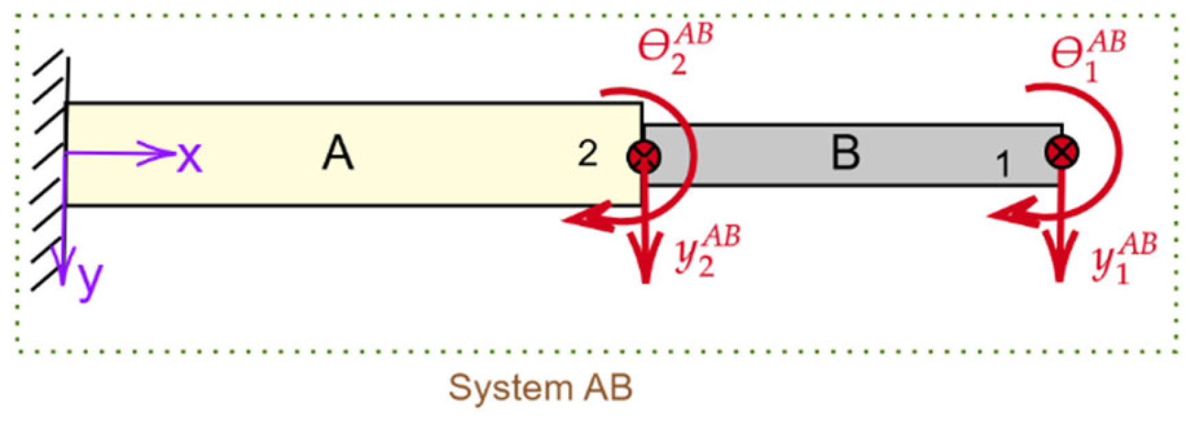
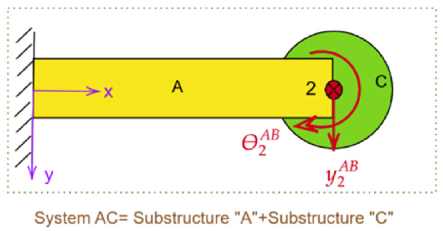
Despite these developments, most generalized receptance coupling methods using FBS either overlook rotational dynamics, leading to inaccuracies, or implicitly include full dynamics, resulting in redundancy in generalized coordinates during the coupling process, particularly at connection points. To address these challenges, this study builds on Jetmundsen’s foundational work, extending GRCFBS to explicitly incorporate rotational DoFs, thereby enhancing the accuracy of system dynamics and synthesizing weak and strong coupling scenarios at interfaces. This explicit approach provides a comprehensive description of the relationship between rotational and translational dynamics, improving system behavior predictions for complex interactions at interfaces and avoiding redundancy issues encountered in methods like LM-FBS. The methodology is demonstrated through two case studies: coupling two flexible components of a cantilever beam and integrating flexible and rigid components.

Additionally, Euler–Bernoulli beam theory (EBT) is employed to derive reduced-order, explicit receptance matrices for substructures, capturing translational and rotational dynamics effectively. This method is particularly valuable for systems like vehicle structures, where moments and forces are applied at connection nodes. While EBT remains a suitable approximation for subsystem modeling, Timoshenko beam theory is recommended for higher-frequency ranges to account for inertial effects and achieve greater accuracy.

Furthermore, EBT is employed to derive reduced-order and explicit receptance matrices for substructures, capturing the full dynamics of both translational and rotational behaviors at DoFs of interest. By explicitly determining the receptance matrix components corresponding to flexible substructures, EBT provides a reliable approximation for both rotational and translational properties at critical points within subsystems. This approach is particularly effective for systems like vehicle structures, where translational forces and moments are applied at nodes, connection points, and coupling regions, accurately accounting for all relevant DoFs within a reduced-order model.

The novelty of this study lies in the development of a practical, generalized formulation for determining the receptance matrix at each substructure node while explicitly incorporating both translational and rotational DoFs (as detailed in Section 2.1). Existing generalized receptance coupling methods, such as those by Jetmundsen, do not fully address the integration of translational and rotational dynamics in their formulations. The explicit definition of rotational dynamics within this framework improves the integrity and comprehensive modeling of the receptance at the critical points, with particular emphasis on connection points, ensuring that both translational and rotational effects are effectively captured. This clarity in system behavior modeling is particularly valuable when addressing complex interactions between substructures. To illustrate this, this paper presents the derivation of receptance coupling formulations for two subsystems, A and B, each with two DoFs (one translational and one rotational). This simplified formulation demonstrates the core mathematical principles without compromising generality or completeness.

For subsystems exhibiting bending and translational dynamics, where experimental receptance data may be unavailable due to measurement challenges, the EBT-based model offers a robust method for estimating the required receptance functions. This capability enables broader applications in structural dynamics and aligns with findings presented in high-speed machining systems (e.g., Schmitz and Duncan, 2005) [15].

The accuracy of the proposed approach is validated through numerical FEA and comparisons of coupled receptance response elements. The alignment of natural frequencies and the identification of resonance and anti-resonance peaks demonstrate consistent and reliable predictions across various excitation conditions. While EBT serves as a reliable approximation for subsystem receptance modeling, Timoshenko beam theory is recommended for higher frequency ranges, where inertial and shear deformation effects become significant for achieving more accurate predictions.

Although this paper focuses on linear systems and modular substructuring, the proposed framework has the potential to be extended to nonlinear systems under certain conditions. Nonlinear joints can be approximated through linearization, and local nonlinear dynamics of substructures can be incorporated as additional dynamic stiffness or represented experimentally as black-box receptance measurements at critical points. These approximations and measurements can then be integrated into the GRCFBS methodology, enabling its application to nonlinear subsystems within a limited range of operating conditions.

2. Methodology

This section presents the methodology for analyzing the dynamic characteristics of mechanical systems using GRCFBS. This approach decomposes complex dynamic systems into simpler substructures, enabling the calculation and analytical coupling of their FRFs. The overall system response is then determined through a generalized coupling algorithm, which effectively combines these subsystems as black boxes carrying receptance matrices. This approach accounts for the interfaces between subsystems. This methodology is evaluated for both flexible-to-flexible and flexible-to-rigid subsystem couplings. Such analysis is essential, as ignoring the flexibility of certain subsystems can introduce significant errors due to incorrect assumptions regarding component rigidity and DoFs. The approach facilitates constructing reduced-order models, where subsystems are modeled by simple geometries, focusing on both rotational and translational DoFs associated with points of interest such as measurement points at connection interfaces or internal points. The inherent properties of each subsystem are incorporated at these points, defined by generalized coordinates in the dynamic model.

This hybrid method aids in predicting vibrational performance for system identification or subsystem decomposition in early development stages, allowing for efficient evaluation of different subsystem combinations. System performance is influenced by the FRF properties of subsystems, which implicitly include stiffness, mass, and damping characteristics, as well as the configuration of coupling and connection joints. Extensive research has demonstrated that the receptance coupling method effectively models vibrations by breaking down complex systems into manageable substructures. The FRFs of these subsystems can be derived experimentally or numerically. To illustrate the analytical solution using GRCFBS, this study simplifies a cantilever beam structure into two substructures, coupled in two ways: first, as a system of two flexible beam elements representing subsystems, and second, as a flexible beam element coupled with a rigid mass. The FRF matrix for flexible subsystems, modeled as simple beam elements, is derived using EBT which assumes small deformations and neglects shear deformation and rotary inertia, making it suitable for linear elastic analysis.

2.1. Review of GRCFBS Methodology

The GRCFBS technique provides a robust framework for coupling receptance matrices of subsystems, derived analytically or experimentally through substructuring methods in the frequency domain. Building on the Jetmundsen formulation [27], this method has been further refined and adapted to suit the specific case studies discussed in this paper. These refinements have introduced innovative equations to facilitate the generalized coupling of multiple subsystems, significantly improving the accuracy of dynamic response predictions. Notably, the sequence in which the FRF matrices are assembled is determined by the number of coordinates involved in the coupling, independent of each subsystem’s DoFs. This method reduces the complexity of the equations needed to describe the entire reconfigurable dynamic system. Fundamentally, the relationship between force excitation (input) and vibration response (output) for a linear system is expressed as follows:

$$\left\{u_p\right\}={\sum }_{q=1}^N\left[H_{pq}\right]\left\{F_q\right\}.$$

(1)

where $\left\{u_p\right\}$ is the vector of the output response at the p-th generalized coordinate or measurement point, $\left\{F_q\right\}$ is the vector of the input excitation force at the q-th generalized coordinate, and $\left[H_{pq}\right]$ represents the component of the receptance matrix between generalized coordinates p and q which may include both rotational and translational DoFs in the general case. The matrix $\left[H_{pq}\right]$ consists of transfer function components that relate the complex rotational or translational displacement amplitudes at measurement points on a dynamic structure to the complex excitation force or moment amplitudes applied at the same or other points, as represented by generalized coordinates. While measuring translational displacements and forces is relatively straightforward, the measurement of rotational displacements and moments presents a greater challenge in dynamic systems. For an arbitrary subsystem, the linear form of the equations of motion, involving direct and indirect receptance components, can be written as follows:

$$\left\{\begin{array}{c}{X}_i\\ X_c\end{array}\right\}=\left[\begin{array}{cc}{H}_{ii}& H_{ic}\\ H_{ci}& H_{cc}\end{array}\right]\left\{\begin{array}{c}{F}_i\\ F_c\end{array}\right\}.$$

(2)

Assuming harmonic force excitation and steady-state responses, the equations governing rotational and translational displacements for a single-node system, across all DoFs, can be expressed as follows:

$$\left\{\begin{array}{c}X\\ Y\\ Z\\ R_x\\ R_y\\ R_z\end{array}\right\}=\left[\begin{array}{cccccc}{H}_{xx}& H_{xy}& H_{xz}& H_{x{r}_x}& H_{x{r}_y}& H_{x{r}_z}\\ H_{yx}& H_{yy}& H_{yz}& H_{y{r}_x}& H_{y{r}_y}& H_{y{r}_z}\\ H_{zx}& H_{zy}& H_{zz}& H_{z{r}_x}& H_{z{r}_y}& H_{z{r}_z}\\ H_{r_{x}x}& H_{r_{x}y}& H_{r_{x}z}& H_{r_x{r}_x}& H_{r_x{r}_y}& H_{r_x{r}_z}\\ H_{r_{y}x}& H_{r_{y}y}& H_{r_{y}z}& H_{r_y{r}_x}& H_{r_y{r}_y}& H_{r_y{r}_z}\\ H_{r_{z}x}& H_{r_{z}y}& H_{r_{z}z}& H_{r_z{r}_x}& H_{r_z{r}_y}& H_{r_z{r}_z}\end{array}\right]\left\{\begin{array}{c}{F}_x\\ F_y\\ F_z\\ M_x\\ M_y\\ M_z\end{array}\right\}.$$

(3)

where x, y, and z are the translational displacements, and $r_x,r_y,\mathrm{a}\mathrm{n}\mathrm{d}{r}_z$ represent the angular displacements about the x, y, and z coordinate axes, respectively. By partitioning Equation (3), the condensed form shown in Equation (4) is obtained:

$$\left\{\begin{array}{c}{u}_t\\ u_r\end{array}\right\}=\left[\begin{array}{cc}{H}_{tt}& H_{tr}\\ H_{rt}& H_{rr}\end{array}\right]\left\{\begin{array}{c}{F}_t\\ F_r\end{array}\right\}.$$

(4)

where $u_t$ and $u_r$ represent the translational and rotational components of displacement, respectively, and $H_{tt}$, $H_{tr}$, $H_{rt}$, and $H_{rr}$ represent the translational response to translational force excitation, translational response to couple excitation, rotational displacement to translational force excitation, and rotational response to couple excitation, respectively.

2.2. Development of General Coupling Formulas with Full DoFs Using GRCFBS

The receptance coupling method, initially formulated by Jetmundsen, describes the coupling of two subsystems (A and B) to yield the assembled subsystem receptance matrix at the interface and internal coordinates, as expressed as follows [8]:

$$\left[\begin{array}{ccc}{H}_{aa}^{AB}& H_{ac}^{AB}& H_{ab}^{AB}\\ H_{ca}^{AB}& H_{cc}^{AB}& H_{cb}^{AB}\\ H_{ba}^{AB}& H_{bc}^{AB}& H_{bb}^{AB}\end{array}\right]=\left[\begin{array}{ccc}{H}_{aa}^A& H_{ac}^A& 0\\ H_{ca}^A& H_{cc}^A& 0\\ 0& 0& H_{bb}^B\end{array}\right]-\left[\begin{array}{c}{H}_{ac}^A\\ H_{cc}^A\\ {-H}_{bc}^B\end{array}\right]{\left[H_{cc}^A+H_{cc}^B\right]}^{-1}\left[\begin{array}{ccc}{H}_{ac}^A& H_{cc}^A& {-H}_{bc}^B\end{array}\right].$$

(5)

In this formulation, subscripts a and b refer to the internal DoFs within substructures A and B, while subscript c corresponds to the connection DoFs between subsystems. In this paper, it is assumed that no internal generalized coordinates within the subsystems are involved, meaning that the points of interest are limited to the connection nodes for simplicity. This assumption does not impact the generality of the procedure. Emphasis is placed on determining $H_{cc}^{AB}$, which captures the direct receptance at the interface based on the individual subsystems’ receptance matrices at the connection coordinates. Under various coupling assumptions, $H_{cc}^{AB}$ can be expanded for two conditions of weak and strong coupling between rotational and translational DoFs at the interfaces. From Equation (5), $H_{cc}^{AB}$ can be expressed in terms of $H_{cc}^A$ and $H_{cc}^B$ as follows:

$$H_{cc}^{AB}={H_{cc}^A-H}_{cc}^A{(H_{cc}^A+H_{cc}^B)}^{-1}{H}_{cc}^A.$$

(6)

Using Equations (4) and (6), the receptance coupling for the assembled system AB can be defined as follows:

$$\left[\begin{array}{cc}{H}_{tt\left(c\right)}^{AB}& H_{tr\left(c\right)}^{AB}\\ H_{rt\left(c\right)}^{AB}& H_{rr\left(c\right)}^{AB}\end{array}\right]=\left[\begin{array}{cc}{H}_{tt\left(c\right)}^A& H_{tr\left(c\right)}^A\\ H_{rt\left(c\right)}^A& H_{rr\left(c\right)}^A\end{array}\right]-\left[\begin{array}{cc}{H}_{tt\left(c\right)}^A& H_{tr\left(c\right)}^A\\ H_{rt\left(c\right)}^A& H_{rr\left(c\right)}^A\end{array}\right]{\left[\begin{array}{cc}{D}_{tt}^{AB}& D_{tr}^{AB}\\ D_{rt}^{AB}& D_{rr}^{AB}\end{array}\right]}^{-1}\left[\begin{array}{cc}{H}_{tt\left(c\right)}^A& H_{tr\left(c\right)}^A\\ H_{rt\left(c\right)}^A& H_{rr\left(c\right)}^A\end{array}\right].$$

(7)

where the matrix D denotes receptance at the connection points and is expressed as follows:

$$\left[\begin{array}{cc}{D}_{tt}^{AB}& D_{tr}^{AB}\\ D_{rt}^{AB}& D_{rr}^{AB}\end{array}\right]=\left[\begin{array}{cc}{H}_{tt\left(c\right)}^A& H_{tr\left(c\right)}^A\\ H_{rt\left(c\right)}^A& H_{rr\left(c\right)}^A\end{array}\right]+\left[\begin{array}{cc}{H}_{tt\left(c\right)}^B& H_{tr\left(c\right)}^B\\ H_{rt\left(c\right)}^B& H_{rr\left(c\right)}^B\end{array}\right].$$

(8)

Assuming a negligible coupling between the translational and rotational DoFs at the connection points between subsystems A and B—meaning that the off-diagonal terms $D_{tr}^{AB}$ and $D_{rt}^{AB}$ in the coupling matrix are approximately zero—the simplified Equation (7) is as follows:

$$\left[\begin{array}{cc}{H}_{tt\left(c\right)}^{AB}& H_{tr\left(c\right)}^{AB}\\ H_{rt\left(c\right)}^{AB}& H_{rr\left(c\right)}^{AB}\end{array}\right]=\left[\begin{array}{cc}{H}_{tt\left(c\right)}^A& H_{tr\left(c\right)}^A\\ H_{rt\left(c\right)}^A& H_{rr\left(c\right)}^A\end{array}\right]-\left[\begin{array}{cc}{H}_{tt\left(c\right)}^A& H_{tr\left(c\right)}^A\\ H_{rt\left(c\right)}^A& H_{rr\left(c\right)}^A\end{array}\right]{\left[\begin{array}{cc}{D}_{tt}^{AB}& 0\\ 0& D_{rr}^{AB}\end{array}\right]}^{-1}\left[\begin{array}{cc}{H}_{tt\left(c\right)}^A& H_{tr\left(c\right)}^A\\ H_{rt\left(c\right)}^A& H_{rr\left(c\right)}^A\end{array}\right].$$

(9)

Due to the principle of reciprocity in dynamic systems, the cross-receptances are equal ($H_{rt\left(c\right)}^A$ = $H_{tr\left(c\right)}^A$) to maintain the symmetry of the system.

The coupling between translational and rotational DoFs at each node is typically weak or negligible under conditions where either the structural or dynamic properties of the connection points or interfaces inherently limit rotational–translational interactions (e.g., pinned connections or hinges), or the physical layout or symmetry of the nodes reduces the likelihood of significant cross-influence. This simplification applies in cases where the stiffness or mass matrix contributions from rotational–translational coupling are minimal, such as in structures with highly localized DoF constraints or when modeling low-frequency dynamics in certain rigid body approximations. Rearranging Equation (9) results in the following:

$${H_{tt\left(c\right)}^{AB}=H_{tt\left(c\right)}^A-H}_{tt\left(c\right)}^A{D_{tt}^{AB}}^{-1}{H}_{tt\left(c\right)}^A-H_{tr\left(c\right)}^A{D_{rr}^{AB}}^{-1}{H}_{rt\left(c\right)}^A.$$

(10)

In Equation (10), the third term, $H_{tr\left(c\right)}^A{D_{rr}^{AB}}^{-1}{H}_{rt\left(c\right)}^A$, represents the effects of the rotational DoFs of the connection points. If only translational DoFs are considered, the equation simplifies to the following:

$${H_{tt\left(c\right)}^{AB}=H_{tt\left(c\right)}^A-H}_{tt\left(c\right)}^A{D_{tt}^{AB}}^{-1}{H}_{tt\left(c\right)}^A.$$

(11)

where ${D_{tt}^{AB}}^{-1}$ and ${D_{rr}^{AB}}^{-1}$ denote the translational and rotational components of dynamic stiffness at the connection area, respectively. For more general scenarios where coupling between rotational and translational DoFs at the interface is significant, the cross-receptance terms, $D_{rt}^{AB}$ and $D_{tr}^{AB}$, of matrix D at the connection zone must be considered, resulting in a more complex form of the equation.

Using the definition of ${{[D}^{AB}]}^{-1}{[D}^{AB}]=[I]$, the inverse matrix ${{[D}^{AB}]}^{-1}={\left[\begin{array}{cc}{D}_{tt}^{AB}& D_{tr}^{AB}\\ D_{rt}^{AB}& D_{rr}^{AB}\end{array}\right]}^{-1}$ can be determined as follows:

$${{[D}^{AB}]}^{-1}=\left[\begin{array}{cc}{\left(D_{tt}^{AB}-D_{tr}^{AB}{D_{rr}^{AB}}^{-1}{D}_{tr}^{AB}\right)}^{-1}& {\left(D_{rt}^{AB}-D_{rr}^{AB}{D_{tr}^{AB}}^{-1}{D}_{tt}^{AB}\right)}^{-1}\\ {{D_{rr}^{AB}}^{-1}{D}_{rt}^{AB}\left(D_{tt}^{AB}-D_{tr}^{AB}{D_{rr}^{AB}}^{-1}{D}_{tr}^{AB}\right)}^{-1}& {{D_{tr}^{AB}}^{-1}{D}_{tt}^{AB}\left(D_{rt}^{AB}-D_{rr}^{AB}{D_{tr}^{AB}}^{-1}{D}_{tt}^{AB}\right)}^{-1}\end{array}\right].$$

(12)

The receptance matrices $H_{tt\left(c\right)}^{AB},H_{tr\left(c\right)}^{AB},H_{rt\left(c\right)}^{AB},\mathrm{a}\mathrm{n}\mathrm{d}{H}_{rr\left(c\right)}^{AB}$ for the coupled system AB are determined for a single node c representing the connection point:

$$\begin{gathered} \left[H_{tt\left(c\right)}\right]=\left[\begin{array}{ccc}{H}_{xx}& H_{xy}& H_{xz}\\ H_{yx}& H_{yy}& H_{yz}\\ H_{zx}& H_{zy}& H_{zz}\end{array}\right],\left[H_{rr\left(c\right)}\right]=\left[\begin{array}{ccc}{H}_{r_x{r}_x}& H_{r_x{r}_y}& H_{r_x{r}_z}\\ H_{r_y{r}_x}& H_{r_y{r}_y}& H_{r_y{r}_z}\\ H_{r_z{r}_x}& H_{r_z{r}_y}& H_{r_z{r}_z}\end{array}\right], \\ \left[H_{rr\left(c\right)}\right]=\left[\begin{array}{ccc}{H}_{r_x{r}_x}& H_{r_x{r}_y}& H_{r_x{r}_z}\\ H_{r_y{r}_x}& H_{r_y{r}_y}& H_{r_y{r}_z}\\ H_{r_z{r}_x}& H_{r_z{r}_y}& H_{r_z{r}_z}\end{array}\right],\left[H_{rt\left(c\right)}\right]=\left[\begin{array}{ccc}{H}_{r_{x}x}& H_{r_{x}y}& H_{r_{x}z}\\ H_{r_{y}x}& H_{r_{y}y}& H_{r_{y}z}\\ H_{r_{z}x}& H_{r_{z}y}& H_{r_{z}z}\end{array}\right]. \end{gathered}$$

(13)

where $H_{xx}$, $H_{xy}$, $H_{yx}$, and $H_{yy}$ represent the coupling parameters for translational DoFs (where the excitation load is a force and the measured displacement is translational), while $H_{r_x{r}_x}$, $H_{r_x{r}_y}$, $H_{r_y{r}_y}$, and $H_{r_z{r}_z}$ represent the coupling parameters for rotational DoFs (where the external excitation is a moment). The terms like $H_{x{r}_x}$, $H_{x{r}_y}$, $H_{y{r}_x}$, and $H_{y{r}_y}$ represent the coupling parameters between translational displacement and rotational excitation load (moment) and vice versa. For simplicity, the coupling of two subsystems A and B, each with two DoFs (one translational and one rotational) has been considered. 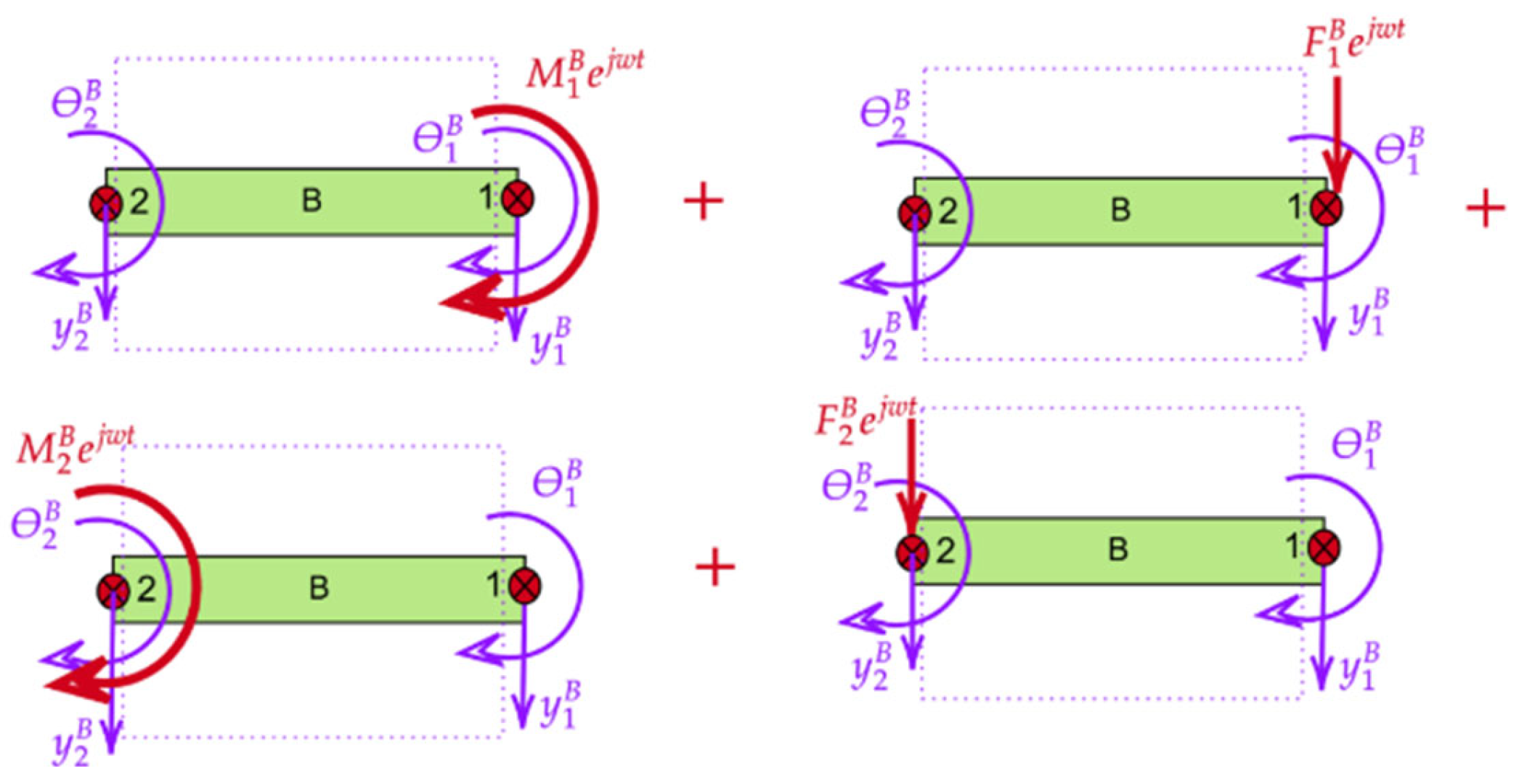For subsystem A, the equation of motion determining the displacement vector of the generalized coordinate ${\mathcal{U}}_2^A$ in terms of the generalized receptance matrix ${\mathcal{H}}_{22}^A$ and the generalized excitation forces $F_2^A$ (including both translational force $F_{y_2}^A$ and moment $F_{{\theta }_2}^A$) can be expressed as follows:

$$\{{\mathcal{U}}_2^A\}=[{\mathcal{H}}_{22}^A{]\{F}_2^A\}\Rightarrow \left\{\begin{array}{c}{y}_2^A\\ {\theta }_2^A\end{array}\right\}=\left[\begin{array}{cc}{H}_{y_2{y}_2}^A& H_{y_2{\theta }_2}^A\\ H_{{\theta }_2{y}_2}^A& H_{{\theta }_2{\theta }_2}^A\end{array}\right]\left\{\begin{array}{c}{F}_{y_2}^A\\ F_{{\theta }_2}^A=M_{{\theta }_2}^A\end{array}\right\}.$$

(14)

For subsystem B, with two generalized coordinates ${\mathcal{U}}_1^B$ and ${\mathcal{U}}_2^B$, the equation of motion can be expressed in terms of the generalized receptance matrices ${\mathcal{H}}_{11}^B,$ ${\mathcal{H}}_{12}^B,{\mathcal{H}}_{21}^B,$ and ${\mathcal{H}}_{22}^B$ and the generalized excitation forces $F_1^B\mathrm{a}\mathrm{n}\mathrm{d}{F}_2^B$:

$$\begin{gathered} \left\{{\mathcal{U}}_1^B\right\}=[{\mathcal{H}}_{11}^B{]\{F}_1^B\}+[{\mathcal{H}}_{12}^B{]\{F}_2^B\}\Rightarrow \left\{\begin{array}{c}{y}_1^B\\ {\theta }_1^B\end{array}\right\}=\left[\begin{array}{cc}{H}_{y_1{y}_1}^B& H_{y_1{\theta }_1}^B\\ H_{{\theta }_1{y}_1}^B& H_{{\theta }_1{\theta }_1}^B\end{array}\right]\left\{\begin{array}{c}{F}_{y_1}^B\\ F_{{\theta }_1}^B\end{array}\right\}+\left[\begin{array}{cc}{H}_{y_1{y}_2}^B& H_{y_1{\theta }_2}^B\\ H_{{\theta }_1{y}_2}^B& H_{{\theta }_1{\theta }_2}^B\end{array}\right], \\ {\{\mathcal{U}}_2^B\}=\left[{\mathcal{H}}_{22}^B\right]{\{F}_2^B\}+[{\mathcal{H}}_{21}^B{]\{F}_1^B\}\Rightarrow \left\{\begin{array}{c}{x}_2^B\\ {\theta }_2^B\end{array}\right\}=\left[\begin{array}{cc}{H}_{y_2{y}_2}^B& H_{y_2{\theta }_2}^B\\ H_{{\theta }_2{y}_2}^B& H_{{\theta }_2{\theta }_2}^B\end{array}\right]\left\{\begin{array}{c}{F}_{y_2}^B\\ F_{{\theta }_2}^B\end{array}\right\}+\left[\begin{array}{cc}{H}_{y_2{y}_1}^B& H_{y_2{\theta }_1}^B\\ H_{{\theta }_2{y}_1}^B& H_{{\theta }_2{\theta }_1}^B\end{array}\right]\left\{\begin{array}{c}{F}_{y_1}^B\\ F_{{\theta }_1}^B\end{array}\right\}. \end{gathered}$$

(15)

Equation (15) can be expressed in the matrix form as follows:

$$\left\{\begin{array}{c}{\mathcal{U}}_1^B\\ {\mathcal{U}}_2^B\end{array}\right\}=\left[\begin{array}{cc}{\mathcal{H}}_{11}^B& {\mathcal{H}}_{12}^B\\ {\mathcal{H}}_{21}^B& {\mathcal{H}}_{22}^B\end{array}\right]\left\{\begin{array}{c}{Q}_1^B\\ Q_2^B\end{array}\right\}.$$

(16)

where $Q_1^B$ and $Q_2^B$ are the generalized excitation forces, expressed as follows:

$$Q_1^B=\left\{\begin{array}{c}{F}_{y_1}^B\\ F_{{\theta }_1}^B\end{array}\right\},Q_2^B=\left\{\begin{array}{c}{F}_{y_2}^B\\ F_{{\theta }_2}^B\end{array}\right\}.$$

(17)

For the assembled system AB, the equation of motion determines the generalized coordinates ${\mathcal{U}}_1^{AB}\mathrm{a}\mathrm{n}\mathrm{d}{\mathcal{U}}_2^{AB}$ in terms of the generalized receptance matrices ${\mathcal{H}}_{11}^{AB},$ ${\mathcal{H}}_{12}^{AB},{\mathcal{H}}_{21}^{AB},$ and ${\mathcal{H}}_{22}^{AB}$, and the generalized excitation forces $Q_1^{AB}$ and $Q_2^{AB}$ can be expressed as follows:

$$\left\{\begin{array}{c}{\mathcal{U}}_1^{AB}={\mathcal{U}}_1^B\\ {\mathcal{U}}_2^{AB}={\mathcal{U}}_2^B\end{array}\right\}=\left[\begin{array}{cc}{\mathcal{H}}_{11}^{AB}& {\mathcal{H}}_{12}^{AB}\\ {\mathcal{H}}_{21}^{AB}& {\mathcal{H}}_{22}^{AB}\end{array}\right]\left\{\begin{array}{c}{Q}_1^{AB}=Q_1^B\\ Q_2^{AB}=Q_2^B\end{array}\right\}.$$

(18)

Assuming rigid coupling between subsystems A and B, the compatibility condition ${{\mathcal{U}}_2^A=\mathcal{U}}_2^B$, and the equilibrium condition at the interface $F_2^A+F_2^B=0$. Using these conditions, the assembly receptance AB can be expressed in terms of the receptance matrices of subsystems A and B as follows:

$$\left\{\begin{array}{c}{\mathcal{H}}_{11}^{AB}={\displaystyle \frac{{\mathcal{U}}_1^{AB}}{F_1^{AB}}}={\displaystyle \frac{{\mathcal{U}}_1^B}{F_1^B}}={\mathcal{H}}_{11}^B-{\mathcal{H}}_{11}^B{\left({\mathcal{H}}_{22}^A+{\mathcal{H}}_{22}^B\right)}^{-1}{\mathcal{H}}_{21}^B,\\ {\mathcal{H}}_{21}^{AB}={\displaystyle \frac{{\mathcal{U}}_2^{AB}}{F_1^{AB}}}={\displaystyle \frac{{\mathcal{U}}_2^B}{F_1^B}}={\mathcal{H}}_{11}^B-{\mathcal{H}}_{11}^B{\left({\mathcal{H}}_{22}^A+{\mathcal{H}}_{22}^B\right)}^{-1}{\mathcal{H}}_{21}^B,\\ {\mathcal{H}}_{22}^{AB}={\displaystyle \frac{{\mathcal{U}}_2^{AB}}{F_2^{AB}}}={\displaystyle \frac{{\mathcal{U}}_2^B}{F_2^B}}={\mathcal{H}}_{22}^A{\left({\mathcal{H}}_{22}^A+{\mathcal{H}}_{22}^B\right)}^{-1}{\mathcal{H}}_{22}^B={\mathcal{H}}_{22}^A-{\mathcal{H}}_{22}^A{\left({\mathcal{H}}_{22}^A+{\mathcal{H}}_{22}^B\right)}^{-1}{\mathcal{H}}_{22}^A,\\ {\mathcal{H}}_{12}^{AB}={\mathcal{H}}_{21}^{AB}.\end{array}\right.$$

(19)

To demonstrate the application of this method, two examples are provided in the following section.

3. Case Studies

The examples presented in this paper are deliberately selected to demonstrate the framework and procedure of the methodology in a clear and structured manner. These examples, such as the beam–node system, enable explicit calculation of stiffness and mass matrices and effectively illustrate the core principles of the method. This simplicity is intentional to ensure that the key features of the methodology are highlighted without introducing unnecessary complexity, making the approach easier to validate against analytical solutions and numerical FEA.

While the examples are simple, they are not meant to fully exhaust the potential of the methodology. Rather, they represent reduced-order approximations of more complex systems. The proposed GRCFBS method is scalable and can effectively analyze systems with intricate geometries by replacing complex substructures with points that carry the corresponding receptance matrix data. This approach allows for the analysis of highly complex systems in a reduced-order form, ensuring that the method remains applicable across a wide range of dynamic systems.

It is important to note that this simple beam–node model can be used as a reduced-order representation to describe a more complex structure [28]. Since this approach is based on coupling receptance matrices at specific points, the complexity of the geometry does not directly influence the methodology. Instead, the complex substructures are effectively replaced by points that carry the receptance matrix data, allowing for the analysis of even highly complex systems in a reduced-order form.

3.1. Case Study 1: Coupling of Continuous Substructures

This case study examines the coupling of two flexible substructures that form a cantilever beam. One substructure is constrained at one end with fixed–free boundary conditions, while the other end remains unconstrained with free–free boundary conditions, as illustrated in Figure 1. The receptance matrix for the entire system matrix is determined using the GRCFBS approach, with components calculated from exact solutions derived from EBT. This method applies receptance coupling at the interface points of these substructures, regardless of whether the boundary conditions are fixed–free or free–free. The method accounts for the dynamic behavior of each subsystem by representing their FRFs or receptance matrices, which fully capture the system’s behavior.

As illustrated in Figure 2, the substructuring strategy decomposes system AB into two substructures A and B.

3.1.1. Determining the Components of Subsystems Receptance

To determine the receptance matrix components for subsystem A, which consists of a flexural beam with fixed–free boundary conditions, we begin with the governing equations derived from EBT [29]. The equation for beam displacement is as follows:

$$EI{\displaystyle \frac{{\partial }^{4}y}{{\partial }^{4}x}}+\rho Ã{\displaystyle \frac{{\partial }^{2}y}{{\partial }^{2}t}}=0.$$

(20)

In this equation, EI, $Ã$, and $\rho$ are flexural rigidity, cross-section area, and density, respectively. This equation assumes that rotary inertia and shear deformations are negligible compared to translational inertia and bending deformations, an approximation valid for slender beams. For free vibration analysis, a steady state (harmonic) solution is assumed where the displacement response in a steady-state is given by $y\left(x,t\right)=Y(x)e^{i\omega t}$. The spatial component $Y\left(x\right)$ can be expressed as follows:

$$Y\left(x\right)=a_1\sin (\lambda x)+a_2\cos (\lambda x)+a_3\sin h(\lambda x)+a_4\cos h(\lambda x).$$

(21)

where ${\lambda }^4={\omega }^2{\displaystyle \frac{\rho Ã}{EI}}$, and $a_1,a_2,a_3,\mathrm{a}\mathrm{n}\mathrm{d}{a}_4$ are coefficients determined by applying the boundary conditions defined in Equation (22) to Equation (21). Here, λ is a parameter related to the natural frequencies and mode shapes of the beam, with $\omega ,\rho ,$ $Ã$, and EI representing the angular frequency, material density, cross-sectional area, and flexural rigidity, respectively. For subsystem A, with fixed–free boundary conditions and with length L, harmonic force and moment excitation are applied at the free end, as shown in Figure 3. The boundary conditions for subsystem A are fixed–free and are specified as follows:

$$y_{\left(x=0\right)}=0,{\theta }_{\left(x=0\right)}={\displaystyle \frac{d{y}_{\left(x=0\right)}}{dx}}=0.$$

(22)

The boundary conditions for subsystem B are free–free and are specified as follows:

$$EI{\displaystyle \frac{d^2{y}_{\left(x=L\right)}}{d^{2}x}}=M_2^A{e}^{i\omega t},EI{\displaystyle \frac{d^3{y}_{\left(x=L\right)}}{d^{3}x}}=0.$$

$$EI{\displaystyle \frac{d^2{y}_{\left(x=L\right)}}{d^{2}x}}=0,EI{\displaystyle \frac{d^3{y}_{\left(x=L\right)}}{d^{3}x}}=-F_{y_2}^A{e}^{i\omega t}.$$

The generalized receptance matrix for subsystem A, with translational and rotational DoFs at the free end, is as follows:

$$[{\mathcal{H}}_{22}^A]=\left[\begin{array}{cc}{H}_{y_2{y}_2}^A& H_{y_2{\theta }_2}^A\\ H_{{\theta }_2{y}_2}^A& H_{{\theta }_2{\theta }_2}^A\end{array}\right].$$

(23)

Each component is determined from receptance definitions and the displacement function $Y\left(x\right)$, given boundary conditions [5,30] as follows:

$$H_{y_2{y}_2}^A={\displaystyle \frac{y_2^A}{F_{y_2}^A}}={\displaystyle \frac{-S_1}{EI{\lambda }^3{S}_8}},H_{y_2{\theta }_2}^A={\displaystyle \frac{y_2^A}{M_2^A}}={\displaystyle \frac{S_2}{EI{\lambda }^2{S}_8}},H_{{\theta }_2{\theta }_2}^A={\displaystyle \frac{{\theta }_2}{M_2^A}}={\displaystyle \frac{S_2}{EI{\lambda }^2{S}_8}.}$$

(24)

where $S_1$ to $S_8$ are defined in Equation (29). For subsystem B, a free–free beam is subjected to forces and moments at both ends, as shown in Figure 4.

The boundary conditions when an excitation couple applies at $x=0$ are the following:

$$EI{\displaystyle \frac{d^2{y}_{\left(x=0\right)}}{d^{2}x}}={-\mathrm{M}}_2^B{e}^{i\omega t},EI{\displaystyle \frac{d^3{y}_{\left(x=0\right)}}{d^{3}x}}=EI{\displaystyle \frac{d^2{y}_{\left(x=L\right)}}{d^{2}x}}=EI{\displaystyle \frac{d^3{y}_{\left(x=L\right)}}{d^{3}x}}=0.$$

(25)

Receptance elements for subsystem B with the same length L are as follows:

$$H_{y_2{\theta }_2}^B={\displaystyle \frac{y_2^B}{M_2^B}}={\displaystyle \frac{-S_2}{EI{\lambda }^2{S}_7},}{H}_{y_1{\theta }_2}^B={\displaystyle \frac{y_1^B}{M_2^B}}={\displaystyle \frac{-S_4}{EI{\lambda }^2{S}_7}},H_{{\theta }_2{\theta }_2}^B={\displaystyle \frac{{\theta }_2^B}{M_2^B}}={\displaystyle \frac{S_5}{EI\lambda S_7}.}$$

(26)

The boundary conditions when an excitation force applies at $x=0$ can be written as follows:

$$EI{\displaystyle \frac{d^2{y}_{\left(x=0\right)}}{d^{2}x}}={\mathrm{F}}_2^B{e}^{i\omega t},EI{\displaystyle \frac{d^3{y}_{\left(x=0\right)}}{d^{3}x}}=EI{\displaystyle \frac{d^2{y}_{\left(x=L\right)}}{d^{2}x}}=EI{\displaystyle \frac{d^3{y}_{\left(x=L\right)}}{d^{3}x}}=0.$$

(27)

The corresponding receptance functions are given by the following:

$$H_{y_2{y}_2}^B={\displaystyle \frac{y_2^B}{F_2^B}}={\displaystyle \frac{{-S}_1}{EI{\lambda }^3{S}_z}},H_{{\theta }_2{y}_2}^B={\displaystyle \frac{{\theta }_2^B}{F_2^B}}={\displaystyle \frac{-S_2}{EI{\lambda }^2{S}_7}}=H_{y_{2{\theta }_2}}^B,H_{y_1{y}_2}^B={\displaystyle \frac{y_1^B}{F_2^B}}={\displaystyle \frac{S_3}{EI{\lambda }^3{S}_7}}=H_{y_2{y}_1}^B,H_{{\theta }_1{\theta }_2}^B={\displaystyle \frac{{\theta }_1^B}{M_2^B}}={\displaystyle \frac{S_6}{EI\lambda S_7}}.$$

(28)

Due to symmetry in the free–free beam, it follows that $H_{{\theta }_2{\theta }_2}^B=H_{{\theta }_1{\theta }_1}^B$, and $H_{y_2{y}_2}^B=H_{y_1{y}_1}^B$.

The terms S1 to S8 used in Equations (24)–(28) are defined as follows:

$$\begin{array}{l}{S}_1=\cos (\lambda L\left)\sin h(\lambda L\right)-\sin (\lambda L\left)\cos h(\lambda L\right),\\ S_2=\sin (\lambda L\left)\sin h(\lambda L\right),S_3=\sin (\lambda L)-\sin h(\lambda L),\\ S_4=\cos (\lambda L)-\cos h(\lambda L),\\ S_5=\cos (\lambda L\left)\sin h(\lambda L\right)+\sin (\lambda L\left)\cos h(\lambda L\right),\\ S_6=\sin (\lambda L)+\sin h(\lambda L),\\ S_7=\cos (\lambda L\left)\cos h(\lambda L\right)-1,\\ S_8=\cos (\lambda L\left)\cos h(\lambda L\right)+1.\end{array}$$

(29)

The parameters S1 to S8 defined in Equation (29) represent the components of the system’s displacement and rotation functions in the context of the boundary conditions and receptance functions [5,31]. These parameters are derived from the solutions to the beam equations under various loading and boundary conditions, and they account for the interaction between the beam’s deflections and rotational displacements.

3.1.2. Numerical FEA for Validation

To validate the receptance matrix obtained using FBS, numerical FEA has been applied. For subsystem A, the stiffness matrix ${[K}_A]$ and mass matrix ${[M}_A]$ are as follows [30,32]:

$$\begin{gathered} {[K}_A]={\displaystyle \frac{{EI}_A}{L_A^3}}\left[\begin{array}{cc}12& -6L_A\\ -6L_A& 4L_A^2\end{array}\right], \\ {[M}_A]={\displaystyle \frac{m_A}{420}}\left[\begin{array}{cc}156& -22L_A\\ -22L_A& 4L_A^2\end{array}\right]. \end{gathered}$$

(30)

It is assumed that both substructures A and B have identical masses, i.e., $m_A=m_B=m.$

Similarly, subsystem B’s stiffness ${[K}_B]$ and mass matrix ${[M}_B]$ are derived as follows:

$$\begin{gathered} {[K}_B]={\displaystyle \frac{{EI}_B}{L_B^3}}\left[\begin{array}{cccc}12& 6L_B& -12& 6L_B\\ 6L_B& 4L_B^2& -6L_B& 2L_B^2\\ -12& -6L_B& 12& -6L_B\\ 6L_B& 2L_B^2& -6L_B& 4L_B^2\end{array}\right], \\ {[M}_B]={\displaystyle \frac{m_B}{420}}\left[\begin{array}{cccc}156& 22L_B& 54& -13L_B\\ 22L_B& 4L_B^2& 13L_B& -3L_B^2\\ 54& 13L_B& 156& -22L_B\\ -13L_B& -3L_B^2& -22L_B& 4L_B^2\end{array}\right]. \end{gathered}$$

(31)

The global mass and stiffness matrix for the assembly AB can then be determined from the following:

$$\begin{gathered} {[K}_{AB}]=\left[\begin{array}{cccc}12({\displaystyle \frac{{EI}_B}{L_B^3}}+{\displaystyle \frac{{EI}_A}{L_A^3}})& 6({\displaystyle \frac{{EI}_B}{L_B^2}}+{\displaystyle \frac{{EI}_A}{L_A^2}})& -12{\displaystyle \frac{{EI}_B}{L_B^3}}& 6{\displaystyle \frac{{EI}_B}{L_B^2}}\\ 6({\displaystyle \frac{{EI}_B}{L_B^2}}+{\displaystyle \frac{{EI}_A}{L_A^2}})& 4({\displaystyle \frac{{EI}_B}{L_B}}+{\displaystyle \frac{{EI}_A}{L_A}})& -6{\displaystyle \frac{{EI}_B}{L_B^2}}& 2{\displaystyle \frac{{EI}_B}{L_B}}\\ -12{\displaystyle \frac{{EI}_B}{L_B^3}}& -6{\displaystyle \frac{{EI}_B}{L_B^2}}& 12{\displaystyle \frac{{EI}_B}{L_B^3}}& -6{\displaystyle \frac{{EI}_B}{L_B^2}}\\ 6{\displaystyle \frac{{EI}_B}{L_B^2}}& 2{\displaystyle \frac{{EI}_B}{L_B}}& -6{\displaystyle \frac{{EI}_B}{L_B^2}}& 4{\displaystyle \frac{{EI}_B}{L_B}}\end{array}\right], \\ {[M}_{AB}]={\displaystyle \frac{1}{420}}\left[\begin{array}{cccc}156(m_B+m_A)& 22{(L}_B{m}_B-L_A{m}_A)& 54& -13L_B\\ 22{(L}_B{m}_B-L_A{m}_A)& 4({m_{A}L}_A^2+{m_{B}L}_B^2)& 13L_B& -3L_B^2\\ 54& 13L_B& 156& -22L_B\\ -13L_B& -3L_B^2& -22L_B& 4L_B^2\end{array}\right]. \end{gathered}$$

(32)

The linear equations of motion for the assembly system AB are expressed as follows:

$$\left\{\begin{array}{c}{y}_2^{AB}\\ {\theta }_2^{AB}\\ y_1^{AB}\\ {\theta }_1^{AB}\end{array}\right\}=[H^{AB}]\left\{\begin{array}{c}{F}_{y_2}^{AB}\\ F_{{\theta }_2}^{AB}\\ F_{y_1}^{AB}\\ F_{{\theta }_1}^{AB}\end{array}\right\}.$$

(33)

where receptance matrix $[H^{AB}]$ of the assembly system AB is determined as follows:

$$[H^{AB}]=\left[\begin{array}{cccc}{H}_{y_2{y}_2}^{AB}& H_{y_2{\theta }_2}^{AB}& H_{y_2{y}_1}^{AB}& H_{y_2{\theta }_1}^{AB}\\ H_{{\theta }_2{y}_2}^{AB}& H_{{\theta }_2{\theta }_2}^{AB}& H_{{\theta }_2{y}_1}^{AB}& H_{{\theta }_2{\theta }_1}^{AB}\\ H_{y_1{y}_2}^{AB}& H_{y_1{\theta }_2}^{AB}& H_{y_1{y}_1}^{AB}& H_{y_1{\theta }_1}^{AB}\\ H_{{\theta }_1{y}_2}^{AB}& H_{{\theta }_1{\theta }_2}^{AB}& H_{{\theta }_1{y}_1}^{AB}& H_{{\theta }_1{\theta }_1}^{AB}\end{array}\right]={[-{\omega }^2[M_{AB}]+[K_{AB}]]}^{-1}.$$

(34)

It is worth noting that in the FBS method, the system is decomposed into two substructures, each with two generalized coordinates and two DoFs. To maintain consistency in the FEA model, each substructure is also modeled as a single beam element with two active nodes and two DoFs. For higher accuracy in FEA, further discretization of each substructure could improve the results.

3.2. Case Study 2: Coupling of a Continuous Substructure and a Rigid Component

To further demonstrate the application of the GRCFBS approach, the second case study investigates the receptance matrix for an assembly system labeled as “AC”. This system is composed of two distinct subsystems: a flexible substructure A and a rigid substructure C, as shown in Figure 5. Substructure A is the same cantilever beam from the first case study, featuring a free–fixed boundary condition, while substructure C is modeled as a rigid body. Both the general receptance method and numerical FEM are applied to solve this problem.

In Figure 6, the decomposition of system AC into substructures A and C using the substructuring technique is shown. Notably, there is only one generalized coordinate at connection point 2, with two DoFs: rotational and translational.

In comparing the two cases, case study 1 involves a combination of two subsystems (A and B) with two generalized coordinates: one at the interface and the other as an internal coordinate of subsystem B. In contrast, case study 2 involves only one generalized coordinate at the connection point from a substructuring perspective, with no internal coordinates. Due to the rigid nature of substructure C, it acts as a lumped mass connected at the interface coordinate ${\mathcal{U}}_2$, exhibiting rigid body motion.

The governing equation for substructure A remains the same as in Equations (22) and (23) from case study 1. The governing equation for substructure C is expressed as follows:

$${\{\mathcal{U}}_2^c\}=\left[{\mathcal{H}}_{22}^c{\left]\right\{F}_2^c\right\}\Rightarrow \left\{\begin{array}{c}{x}_2^c\\ {\theta }_2^c\end{array}\right\}=\left[\begin{array}{cc}{H}_{y_2{y}_2}^c& H_{y_2{\theta }_2}^c\\ H_{{\theta }_2{y}_2}^c& H_{{\theta }_2{\theta }_2}^c\end{array}\right]\left\{\begin{array}{c}{F}_{y_2}^c\\ F_{{\theta }_2}^c=M_{{\theta }_2}^c\end{array}\right\}.$$

(35)

where $\left[{\mathcal{H}}_{22}^c\right]$ represents the receptance matrix for substructure C, and $F_{y_2}^c$ and $F_{{\theta }_2}^c(M_{{\theta }_2}^c)$ are the force and moment excitations applied. As illustrated in Figure 7, excitation loads (force and moment) are applied separately to substructure C to determine the translational and angular displacements. The receptance components relating displacements to excitation loads are given by the following:

$$H_{y_2{y}_2}^c={\displaystyle \frac{-1}{m_B{\omega }^2}},H_{y_2{\theta }_2}^c=H_{{\theta }_2{y}_2}^c=0,H_{{\theta }_2{\theta }_2}^c={\displaystyle \frac{-1}{I_c{\omega }^2}}.$$

(36)

where $I_c$ and $m_c$ are the moment of inertia and mass of the rigid wheel as substructure C, respectively. When a harmonic force $F_{y_2}^c{e}^{i\omega t}$ and $M_{{\theta }_2}^c{e}^{i\omega t}$ are applied to this rigid component, the assembly system AC is excited. The motion of the free end of the beam can be analyzed by considering both the beam’s flexural response and the inertia of the rigid body. Since substructure C has no internal DoFs or generalized coordinates, the coupling equation for calculating the receptance function of the assembly AC is determined from the receptance components at the connection point using generalized receptance coupling:

$${\mathcal{H}}_{22}^{AC}={\displaystyle \frac{{\mathcal{U}}_2^{AC}}{F_2^{AC}}}={\displaystyle \frac{{\mathcal{U}}_2^C}{F_2^C}}={\mathcal{H}}_{22}^A{\left({\mathcal{H}}_{22}^A+{\mathcal{H}}_{22}^C\right)}^{-1}{\mathcal{H}}_{22}^B={\mathcal{H}}_{22}^A-{\mathcal{H}}_{22}^A{\left({\mathcal{H}}_{22}^A+{\mathcal{H}}_{22}^C\right)}^{-1}{\mathcal{H}}_{22}^A.$$

(37)

Here, the receptance matrix for system AC is a 2 × 2 matrix, expressed as follows:

$$[H^{AC}]=\left[\begin{array}{cc}{H}_{y_2{y}_2}^{AC}& H_{y_2{\theta }_2}^{AC}\\ H_{{\theta }_2{y}_2}^{AC}& H_{{\theta }_2{\theta }_2}^{AC}\end{array}\right].$$

(38)

4. Results and Discussion

This section presents and analyzes the results from the receptance analysis of two case studies, Figure 2 and Figure 6, with a focus on validating the GRCFBS method against FEA. This comparative simulation is conducted in MATLAB (2023b) using the theoretical approaches using the parameters discussed here. The findings provide insights into the dynamic behavior of coupled systems and highlight the accuracy and limitations of the proposed method under different structural configurations.

Table 1. Subsystem parameters for modeling purposes.

Parameter	Description	Unit	Substructure
			A	B	C
			Fixed–Free Beam	Free–Free Beam	Rigid Wheel
E	Elastic modulus	N/m2	200× 109	200× 109
I	Moment of inertia	kgm2	3.4× 10−7	3.4× 10−7	1.9× 10−8
EI	Flexural rigidity	Nm2	7.5× 108	3.8× 103
L	Length	m	0.25	0.15
A	Cross-section area	m2	2× 10−3	5× 10−4
$\rho$	Density	kg/m3	7800	7800
m	Mass	kg	3.90	$0.57$	0.57

summarizes the parameters for the modeling of the subsystems, including elastic properties, geometric dimensions, and mass for each substructure used in the case studies.

For each case study, the synthesis of the receptance matrix components derived from GRCFBS using EBT is compared to FEA results for both direct and cross-receptance.

4.1. Case Study 1: Flexible Beam Coupling

In the first case, involving the coupling of two flexible beams (assembly system AB), the direct/cross-receptance matrix components were evaluated at the tip ${\mathcal{U}}_1$ and connection point ${\mathcal{U}}_2$. The results of the theoretical works outlined in Section 3.1 and shown in Figure 8, Figure 9, Figure 10 and Figure 11 demonstrate GRCFBS’s ability to capture the dynamic interactions between substructures, with close alignment to FEA at the primary vibrational modes.

4.1.1. Direct Receptance Components at Node with Generalized Coordinate ${\mathcal{U}}_1$

The direct components of receptance matrix ${[H}^{AB}]$ of the coupled system AB at the tip node with generalized coordinate ${\mathcal{U}}_1$—$H_{y_1{y}_1}^{AB},H_{y_1{\theta }_1}^{AB},\mathrm{a}\mathrm{n}\mathrm{d}{H}_{{\theta }_1{\theta }_1}^{AB}$—are represented in Figure 8, Figure 9 and Figure 10, comparing the magnitudes of these components. Notably, $H_{{\theta }_1{y}_1}^{AB}$ is omitted due to reciprocity, i.e., $H_{{\theta }_1{y}_1}^{AB}=H_{y_1{\theta }_1}^{AB}$.

Figure 8 shows $H_{y_1{y}_1}^{AB}$, the translational displacement at the tip caused by a translational excitation force applied at the same location. The FEA and GRCFBS results closely match for the primary two natural frequencies. For the first mode, FEA estimates the first mode at 368.1 Hz and GRCFBS at 383 Hz, a 3.8% increase, reflecting the stiffer response captured by the GRCFBS method. For the second mode, FEA predicts 1020.9 Hz, while GRCFBS gives 1025.7 Hz, resulting in a minor 0.4% difference, which is much less significant. Despite these small discrepancies in natural frequencies, it is important to highlight that the GRCFBS results show slightly reduced amplitude at dominant modes compared to FEA. This can be attributed to the continuous (distributed) nature of the system of the system in GRCFBS, which inherently suggests a stiffer system and, therefore, results in a reduced response amplitude. In the context of the EBT used in the GRCFBS method, each beam is treated as a continuous element, providing a simplified solution that may not fully account for flexibility at higher frequencies. Given that the system (AB) has four DoFs, four peaks are expected, but only two natural frequencies fall within the range up to 3000 Hz. Near 3000 Hz, GRCFBS shows an anti-resonance not captured by FEA. Up to 2000 Hz, the receptance component—i.e., the relationship between the applied force and resulting displacement—shows good agreement between FEA and GRCFBS, particularly in the lower-frequency regime where both methods perform similarly. However, as the frequency increases beyond 2000 Hz, discrepancies begin to grow, primarily due to the limitations of the beam model theory used in both numerical FEA and GRCFBS at high frequencies. At these higher frequencies, inertial effects and material damping become increasingly important, but are not fully accounted for in the current model, leading to increased divergence between the two methods. Figure 9 displays the receptance component $H_{y_1{\theta }_1}^{AB}$, showing the translational displacement at the tip resulting from a couple applied at the same location. Both methods demonstrate similar trends in the resonance and anti-resonance peaks of the receptance component $H_{y_1{y}_1}^{AB}$, as illustrated in Figure 8. Notably, a frequency shift is observed beyond 2000 Hz. This shift indicates an increase in stiffness in the FEA response, likely due to higher-order effects that are more pronounced in FEA. However, it is important to note that both methods encounter limitations when modeling high-frequency dynamics, where inertia effects become increasingly dominant. These effects, including shear deformation and rotational inertia, are not adequately captured by the assumptions in EBT, which is used in the GRCFBS method. Similarly, the beam models employed in FEA—which rely on stiffness and mass matrices and the coupling between stiffness and mass at nodes—also fail to fully account for these higher-frequency phenomena. As a result, both methods may misrepresent the system’s true behavior at these elevated frequencies, particularly where inertia effects play a significant role.

In Figure 10, the receptance component $H_{{\theta }_1{\theta }_1}^{AB}$, representing the rotational displacement at the tip due to a rotational moment applied at the same location, shows a strong alignment between the GRCFBS and FEA methods across all frequencies. Both methods accurately capture the resonance and anti-resonance peaks, suggesting that the EBT is effective in modeling the system’s rotational dynamics within the frequency range considered. This alignment is particularly notable because rotational displacement under a rotational moment is well captured, indicating that EBT sufficiently models the bending resistance and rotational behavior of the system, which dominates in this frequency range.

When comparing this result with Figure 8 and Figure 9, the key difference emerges in how each method handles translational displacement responses. In Figure 8, which represents translational displacement due to a translational force, both methods align well up to approximately 2000 Hz, but discrepancies start to appear as the frequency increases, primarily due to limitations in accurately capturing high-frequency inertia effects and shear deformation. Similarly, in Figure 9, which shows the translational displacement response due to a rotational moment, both methods match closely in the primary modes, but a slight frequency shift in FEA suggests a softer structure with increased deformation amplitude, especially at higher frequencies.

However, in Figure 10, the rotational displacement response under a rotational moment does not show such discrepancies, and both methods remain in strong agreement across the entire frequency range, even beyond 2000 Hz. This observation is significant because it highlights the different behavior of rotational dynamics compared to translational dynamics. Rotational dynamics, such as the response captured in Figure 10, are less influenced by higher-order effects like inertia and shear deformation, which primarily affect translational displacement responses (as seen in Figure 8 and Figure 9).

Thus, while Figure 8 and Figure 9 show discrepancies between the GRCFBS and FEA methods at higher frequencies due to the limitations of both models in capturing inertia effects and shear deformation, Figure 10 demonstrates a consistent alignment in rotational displacement responses, suggesting that the EBT is well-suited for modeling rotational behavior even at higher frequencies. This reinforces the idea that while translational dynamics are more sensitive to high-frequency phenomena, the rotational dynamics remain well-modeled across the frequency range considered.

A comparison of the receptance components ${H_{y_1{y}_1}^{AB},H_{y_1{\theta }_1}^{AB},\mathrm{a}\mathrm{n}\mathrm{d}H}_{{\theta }_1{\theta }_1}^{AB}$ over an expanded frequency range up to 6000 Hz, covering all four modes, is presented in Figure 11. Despite differences in values arising from the specific nature of the excitation and response, resonance frequencies remain consistent across various excitation types, reinforcing their status as intrinsic system characteristics. This consistency indicates that the resonance frequencies predicted by the different excitations—whether translational force or rotational moment— remain consistent. Such alignment underscores that natural frequencies are inherent properties of the system and remain unaffected by the type of excitation applied.

4.1.2. Direct Receptance Components at Connection Point (Node ${\mathcal{U}}_2$)

Understanding the receptance components at the connection point is crucial for assessing the dynamic behavior of the system, particularly where interactions between substructures occur. These components form a critical part of the overall receptance matrix, as they effectively capture the coupling dynamics between substructures. The accuracy of the connection receptance matrix, however, can be highly sensitive to perturbations such as noise or numerical errors. This sensitivity arises from the inverse operations inherent in the generalized coupling formula, as well as the receptance properties at the connection points, which are influenced by the individual substructures’ dynamic characteristics. Accurately modeling these receptance components is, therefore, essential for ensuring reliable predictions of the system’s overall behavior.

In Figure 12, the receptance component $H_{y_2{y}_2}^{AB}$ is presented, representing the translational displacement at the connection point caused by an applied excitation force at the same location. The results demonstrate a similar trend and level of accuracy observed in the tip node $H_{y_1{y}_1}^{AB}$ (Figure 8) between the GRCFBS and FEA methods. This suggests that, even at the critical point of connection between two substructures, both methods can effectively capture the primary translational dynamics within the system. This consistency may arise from how well the compatibility and equilibrium boundary conditions at the connection point are incorporated into the GRCFBS approach.. Furthermore, the translational dynamics at the connection point are less influenced by higher-order effects like rotational coupling which can be observed in the result.

Figure 13 illustrates the cross-receptance component $H_{y_2{\theta }_2}^{AB}$, which represents the translational displacement induced by applying a rotational moment at the connection point. Interestingly, this cross-receptance exhibits an even stronger correlation between the methods than was observed for the corresponding tip response in $H_{y_1{\theta }_1}^{AB}$ (Figure 9). Both methods effectively predict resonance and anti-resonance peaks within the 0–3000 Hz range, demonstrating robust performance in modeling the coupling dynamics between translational and rotational motions.

Figure 14 illustrates the receptance component $H_{{\theta }_2{\theta }_2}^{AB}$ at the connection point, representing the rotational displacement caused by an applied excitation couple at the same location. The correlation between the GRCFBS and FEA methods is robust, closely aligning with the results observed for the tip node $H_{{\theta }_1{\theta }_1}^{AB}$ (Figure 10). This strong agreement highlights the ability of both methods to effectively capture the rotational dynamics at the connection point, a critical interface where the coupling of substructures can influence system behavior. The similarity in trends suggests that the EBT (as used in GRCFBS) is capable of accurately modeling rotational dynamics at these connection points within the analyzed frequency range. Additionally, this consistency underscores the reliability of the GRCFBS approach in handling rotational degrees of freedom, even in regions where the interaction between substructures could introduce additional complexities.

Finally, Figure 15 compares $H_{y_2{y}_2}^{AB},H_{y_2{\theta }_2}^{AB},\mathrm{a}\mathrm{n}\mathrm{d}{H}_{{\theta }_2{\theta }_2}^{AB}$ across a higher frequency range up to 6000 Hz to capture all four modes. Despite variations in response characteristics, the alignment on natural frequency peaks indicates consistent resonance predictions across different excitation conditions, like the observations at the tip node shown in Figure 11.

4.1.3. Cross-Receptance Components Between Tip and Connection Point

Cross-receptance components reflect the dynamic coupling effects between different nodes in the system and play a pivotal role in validating the accuracy of the model’s representation of system interactions. These components are essential for achieving a comprehensive understanding of the system’s dynamic behavior. They assist in validating models, optimizing designs, and diagnosing performance characteristics by highlighting how forces or moments at one node influence displacements at another. The following figures illustrate the variations and correlations observed in these components.

Figure 16 illustrates the cross-receptance component $H_{y_2{y}_1}^{AB}$, which represents the translational displacement at the tip node caused by a force applied at the connection point. Unlike previous receptance components, no anti-resonance is observed between the first two dominant resonant peaks. However, one anti-resonance appears after the second resonant peak. This behavior is effectively captured by the GRCFBS, the same as the FEA method, demonstrating strong alignment in characterizing this dynamic feature, particularly around the 2000 Hz frequency range. The absence of an anti-resonance between the first two dominant peaks can be attributed to the nature of the force transmission between the tip and the connection point in this specific cross-receptance case. Since the force is applied directly at the connection node, the coupling between the substructures is predominantly influenced by translational dynamics, which tend to smooth out higher-order oscillatory effects like anti-resonances in this frequency range. This results in a more direct interaction between the two resonant modes, without significant modal interference that would typically produce an anti-resonance.

The appearance of an anti-resonance after the second resonant peak can be explained by the interaction of higher-order modes, where rotational and translational coupling effects become more pronounced. At this frequency, the dynamic behavior of the system introduces phase cancellations between the input force and the system’s response, leading to the anti-resonance. Both the GRCFBS and FEA methods successfully capture this characteristic, reinforcing their ability to model complex dynamic interactions at the connection node. Additionally, the accuracy observed around the 2000 Hz range highlights the robustness of the GRCFBS method in matching the benchmark FEA approach for the primary modes of interest. The consistent alignment of natural frequencies and the ability to replicate anti-resonance features validate the GRCFBS methodology as a reliable tool for analyzing cross-receptance dynamics, even in scenarios with nuanced interactions like this one.

Figure 17 and Figure 18 illustrate the indirect receptance components $H_{y_2{\theta }_1}^{AB}$ and $H_{{\theta }_2{\theta }_1}^{AB}$, representing the translational and rotational displacements, respectively, at the connection node caused by an excitation couple at the tip. Both graphs exhibit trends similar to those observed in Figure 16, particularly in terms of the resonance and anti-resonance regimes.

For $H_{y_2{\theta }_1}^{AB}$, the interaction highlights how rotational excitation at the tip is transmitted to induce translational dynamics at the connection node. Likewise, $H_{{\theta }_2{\theta }_1}^{AB}$ demonstrates the rotational response at the connection node due to the same tip excitation. The results indicate a very strong correlation between the GRCFBS and FEA methods across the entire frequency range analyzed, particularly up to 2000 Hz. This alignment suggests that both methods are highly effective in capturing the system’s coupled dynamic response within the dominant frequency modes. The trends in Figure 18 for $H_{{\theta }_2{\theta }_1}^{AB}$ closely resemble those observed in rotational receptance components $H_{{\theta }_1{\theta }_1}^{AB}$ and $H_{{\theta }_2{\theta }_2}^{AB}$, further confirming the consistency between the two methodologies. Both the GRCFBS and FEA approaches effectively replicate the rotational coupling dynamics, maintaining strong correlations in both resonance peaks and anti-resonance behavior across the frequency range. The similarity in behavior across these indirect receptance components underscores the ability of the GRCFBS method to capture coupled dynamics between rotational and translational degrees of freedom. This is particularly important because such dynamics are often more challenging to model due to the interplay of higher-order effects and phase relationships in coupled systems.

Additionally, the consistency observed in the alignment of natural frequencies and resonance peaks further validates the robustness of the GRCFBS method and reinforces the suitability of this approach as a reduced-order alternative to FEA for dynamic modeling of complex coupled systems.

A comparison has been made between $H_{y_1{y}_2}^{AB},H_{y_1{\theta }_2}^{AB},\mathrm{a}\mathrm{n}\mathrm{d}{H}_{{\theta }_1{\theta }_2}^{AB}$ for the higher frequency range up to 6000 Hz, covering all four mode shapes and peaks, as shown in Figure 19. Regardless of variations in response characteristics, the alignment on natural frequency peaks indicates consistent resonance predictions across different excitation conditions, like the observations at the tip and connection nodes.

4.2. Case Study 2: Flexible Beam–Rigid Wheel Coupling

In this case study, the receptance components of the assembly system AC, which couples a flexible beam with a rigid wheel, have been analyzed. The assembly system is illustrated in Figure 5 and Figure 6. The primary objective is to evaluate how the interaction between the flexible and rigid substructures influences dynamic behavior and the receptance characteristics of the coupled system. In this configuration, the tip and the connection point (node ${\mathcal{U}}_2$) are coincident, eliminating the distinct $H_{y_1{y}_1}^{AC}$ component.

The receptance components are calculated using the theoretical approaches outlined in Section 3.2. For this analysis, the stiffness of the rigid wheel is neglected, resulting in a global stiffness matrix for the assembly (AC) that remains consistent with that of substructure A. Substructure C incorporates an inertia matrix without any stiffness in FEA. However, in the GRCFBS method, substructure C incorporates an FRF matrix accounting for both translational and rotational inertia. The coupled system AC exhibits two dominant modes due to the inclusion of a single generalized coordinate with two DoFs. Figure 20, Figure 21, Figure 22 and Figure 23 illustrate the receptance components for this assembly.

Figure 20 presents the direct receptance component $H_{y_2{y}_2}^{A\mathrm{C}}$, representing the translational displacement at node U₂; due to an applied excitation force. The results indicate that the rigid wheel’s lack of stiffness significantly reduces system stiffness, leading to a shift in natural frequencies and altering the dynamic response. The GRCFBS method predicts the first mode at 483 Hz, while the FEA method predicts it at 468 Hz, reflecting a slight increase in effective stiffness (approximately 3%). This alignment demonstrates strong agreement between the two methods for the first dominant mode. However, deviations are observed at higher frequencies, particularly beyond 2000 Hz, where the influence of the rigid component becomes increasingly pronounced.

These higher-frequency discrepancies are attributed to the growing dominance of inertia effects and the role of stiffness at connection points in the GRCFBS method. The accuracy of the GRCFBS method hinges on the precision of receptance coupling at the interface, which is influenced by stiffness, mass, and damping parameters. When the stiffness contribution of one substructure is omitted, as in the rigid wheel model, inherent errors arise in predicting the system’s dynamic response. These errors become more evident at higher frequencies, where the receptance coupling mechanism is less effective. In contrast, the inclusion of stiffness contributions at connection points, as in case study 1, enhances the correlation between GRCFBS and FEA, particularly for systems with significant stiffness at the connection interface. This underscores the critical role of stiffness in improving the accuracy of receptance coupling predictions.

Figure 21 and Figure 22 depict the cross-receptance components $H_{y_2{\theta }_2}^{AC}$ and $H_{{\theta }_2{\theta }_2}^{AC},$ capturing the coupling between translational and rotational dynamics at the coincident tip/connection point due to applying an excitation moment. These components highlight the role of rotational stiffness introduced by the rigid wheel. The presence of anti-resonances, unique to this flexible–rigid coupling, indicates constrained vibrational modes that affect energy transfer within the system. Like $H_{y_2{y}_2}^{AC}$, there is good agreement between the two methods up to 2000 Hz for the first dominant mode, and the discrepancy appeared for the second mode at higher frequencies.

Figure 23 compares $H_{y_2{y}_2}^{A\mathrm{C}},H_{y_2{\theta }_2}^{A\mathrm{C}},\mathrm{a}\mathrm{n}\mathrm{d}{H}_{{\theta }_2{\theta }_2}^{A\mathrm{C}}$ for a higher frequency range up to 6000 Hz to cover two modes. While the magnitude of these components varies due to the nature of the system and the excitation applied, all three receptance components align at the natural frequency peaks. This alignment indicates that the resonance frequencies predicted by the three receptance components, despite different excitations, remain consistent, as seen in the previous case. This consistency suggests that whether considering translational or rotational excitations, the predicted natural frequencies are stable, as natural frequencies are intrinsic properties of the system.

Figure 24 provides a comparative analysis of the receptance component at the tip, specifically translational displacement due to an excitation force, for two distinct configurations: the beam–beam setup and the beam–rigid wheel configuration. Using the GRCFBS method, this comparison reveals notable differences in dynamic behavior between the two systems in spite of similar mass between substructures B and C. In the beam–beam configuration, the system exhibits four resonance peaks, indicative of a more complex dynamic response due to the combined stiffness contributions of both beams. In contrast, the beam–rigid wheel configuration demonstrates only two natural frequencies, reflecting a simpler dynamic behavior due to the contribution of only one beam stiffness and the rigid wheel’s inertia contribution.

The peak magnitudes in the beam–beam setup are higher compared to the beam-rigid wheel configuration, suggesting that the beam–beam coupling results in a softer system with reduced overall stiffness. This indicates that the beam–beam coupling experiences greater flexibility and higher peak responses under excitation compared to the beam–rigid wheel setup.

It is worth noting that the frequency range up to 2000 Hz is generally considered high for large mechanical systems, such as those typically analyzed in automotive engineering where NVH focuses on frequencies from 0 to 1000 Hz, with some analysis extending to around 2000 Hz. However, for smaller, high-speed systems such as turbines and motors, higher frequencies can be more relevant.

Table 2. Comparison of dominant modes of vibration for GRCFBS and FEA methods below 2000 Hz.

Case Study	Mode	Receptance Component	GRCFBS	FEA	Error %
1 (AB)	Resonance		383.1 1025.7	368.1 1020.9	3.8 0.4
	Anti-resonance	$H_{y_1{y}_1}^{AB}$	688.8	673.3	2.3
		$H_{y_2{y}_2}^{AB}$	756	754.2	0.24
		$H_{y_1{\theta }_2}^{AB}$	1219.7	1186.7	2.78
		$H_{{\theta }_1{\theta }_1}^{AB}$	438.3 1448.4	421.2 1466.3	4.06 1.22
		$H_{y_2{\theta }_2}^{AB}$	1733.9	1792.7	3.28
		$H_{{\theta }_2{\theta }_2}^{AB}$	682.8 1042.4	672 1056.3	1.61 1.33
2 (AC)	Resonance		483	468	3
	Anti-resonance	$H_{{\theta }_2{\theta }_2}^{AB}$	839.5	807.1	4.01
		$H_{y_2{\theta }_2}^{AB}$	1733.9	1792.7	3.28

provides a comparative analysis of dominant modes of vibration for case studies 1 and 2 (systems AB and AC) in terms of resonance and anti-resonance frequencies below 2000 Hz. The receptance components and the associated percentage errors are listed to evaluate the accuracy of the GRCFBS method against the FEA benchmark. The results highlight the strengths and limitations of GRCFBS in predicting translational and rotational motions across different dynamic coupling scenarios.

5. Limitations

While the GRCFBS method provides a reliable approximation of system vibrational characteristics, several limitations affect its accuracy at higher frequencies.

• Euler–Bernoulli beam theory (EBT) assumptions: the Euler–Bernoulli beam theory used in the current analysis assumes negligible shear deformation and rotational inertia. At higher frequencies, these assumptions become less valid, which leads to discrepancies in the predicted magnitudes of the resonance peaks. This limitation is particularly relevant for systems operating at higher frequencies (above 2000 Hz), where rotational inertia and shear effects are more significant;
• Absence of material damping: the model does not include material damping, which plays a critical role in attenuating vibrations at high frequencies;
• Alternative beam theories: to improve accuracy at higher frequencies, future work could incorporate alternative beam theories, such as the Timoshenko beam theory, which accounts for shear deformation and rotational inertia. Additionally, including material damping in future models would help more accurately reflect the behavior of real-world systems at high frequencies;
• High-frequency behavior and inertia effects: both the FEA and GRCFBS methods exhibit a noticeable frequency shift beyond 2000 Hz, suggesting that higher-order effects are more pronounced in the FEA results. However, both methods encounter limitations when modeling high-frequency dynamics, where inertia effects (such as shear deformation and rotational inertia) become dominant. These effects are not fully captured by the assumptions in the EBT or the beam models used in FEA, which could lead to misrepresentations of the system’s true behavior at higher frequencies;
• Rotational receptance accuracy beyond 2000 Hz: despite the observed discrepancies in magnitude, the rotational receptance (both direct and cross components) shows good agreement for frequencies beyond 2000 Hz. This indicates that while the methods may not fully capture the magnitude of the system’s vibrational response at high frequencies, they remain consistent in predicting the resonance frequencies where rotational effects are more pronounced.

6. Conclusions

This study evaluates the effectiveness and limitations of the GRCFBS method, which integrates generalized receptance coupling with FBS approaches. By developing explicit rotational DoFs, this approach improves the prediction accuracy of dynamic systems that experience both translational and rotational motions. Building on Jetmundsen’s foundational work, the proposed framework introduces a practical, generalized formulation that explicitly incorporates full translational and rotational dynamics at each substructure node. This explicit formulation accounts for both translational and rotational displacements, enhancing the model’s capability to predict the dynamic behavior of coupled systems more efficiently. The refinement of the GRCFBS method, which integrates rotational DoFs into the system formulation, provides a more comprehensive approach to capturing the dynamics of flexible structures and their interactions under complex loading conditions.

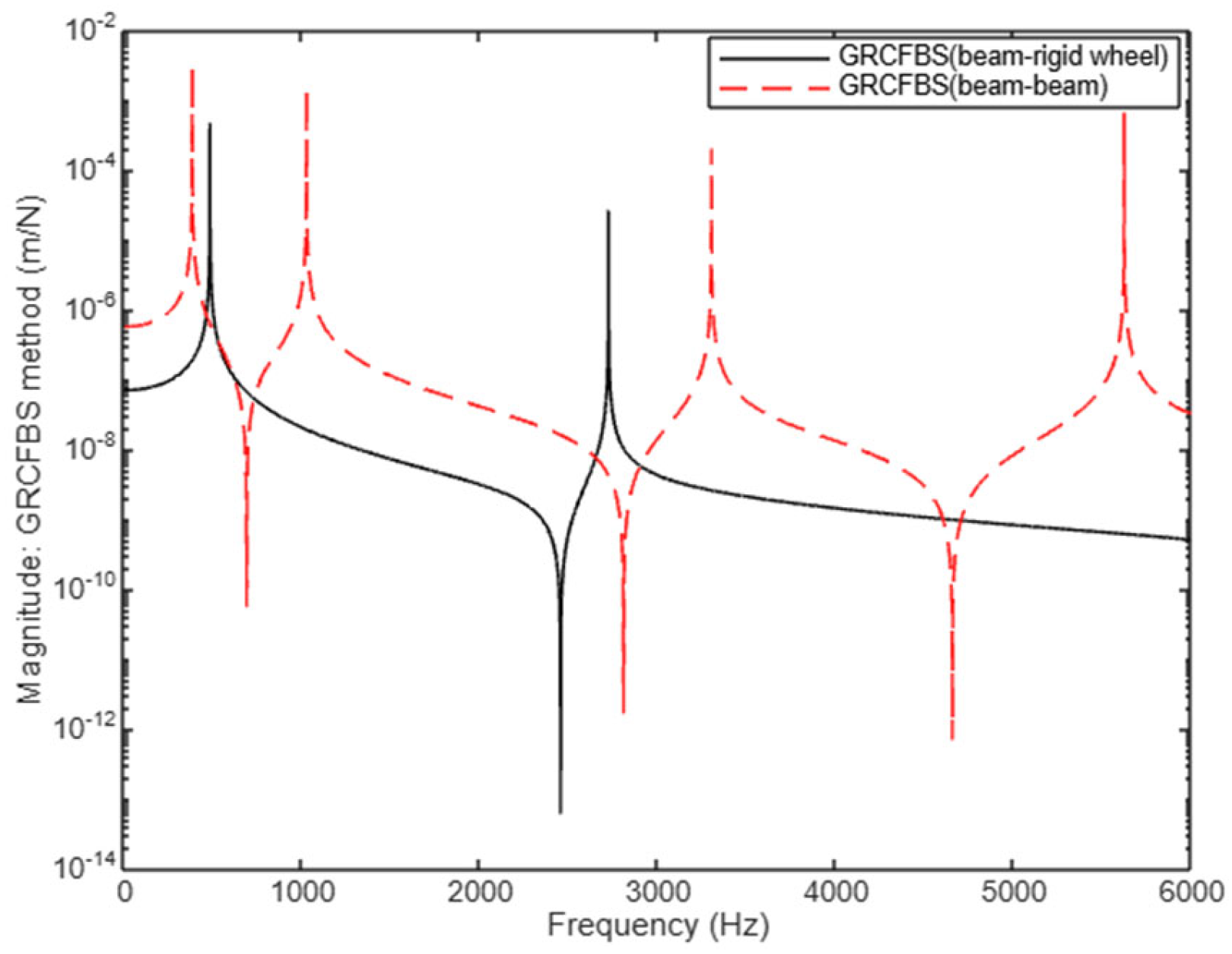
This study focuses on two case studies: a flexible beam–beam coupling and a flexible beam–rigid wheel coupling, validating the performance of the GRCFBS method in these configurations.

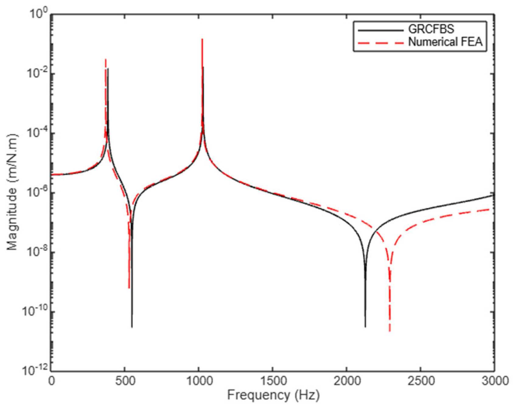
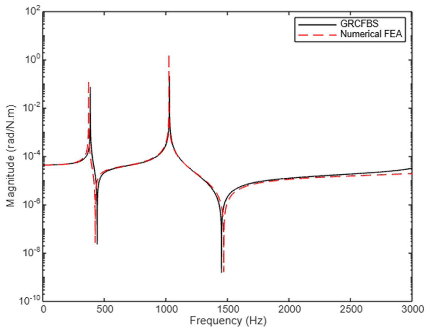
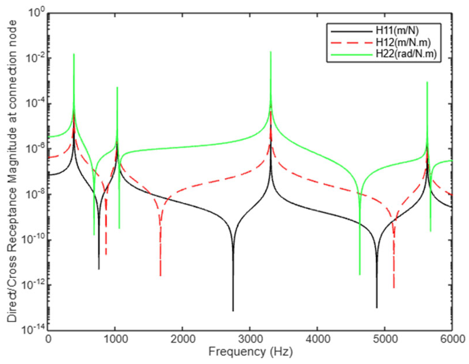
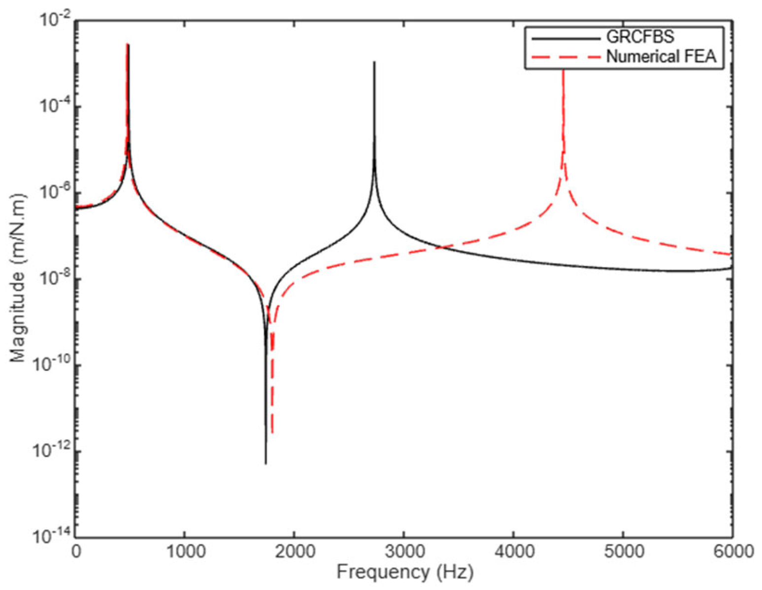
The results demonstrate that the GRCFBS method, when employing the EBT, accurately predicts system vibrational characteristics, especially at a lower range of frequencies (up to 2000 Hz), where it shows strong alignment with FEA. Specifically, the relative error in predicting resonance frequencies at lower frequencies is found to be less than 5%, indicating a high degree of accuracy for these ranges. Both direct and cross-receptance components show good agreement in predicting natural frequencies and dynamic responses. In the case of the beam–beam coupling, the presence of four resonance peaks and the higher response magnitudes are attributed to the inclusion of both translational and rotational DoFs, providing more complex dynamic behavior.

While the GRCFBS method demonstrates strong agreement with FEA for both resonance and anti-resonance frequencies below 2000 Hz (with errors typically below 5%), discrepancies become apparent at higher frequencies (above 2000 Hz), where the accuracy decreases, resulting in relative errors exceeding 10% for non-rotational receptances. These discrepancies highlight the need for refinement of the theory of node receptance description in GRCFBS and the use of more accurate beam elements in FEA. Such advancements could better capture higher-order dynamic behaviors and further enhance the predictive accuracy of the method in these frequency ranges.

However, both the FEA and GRCFBS methods exhibit similar trends in resonance and anti-resonance peaks, with a noticeable frequency shift observed beyond 2000 Hz.

As an interesting observation, the rotational receptance components (both direct and cross) maintain a good agreement beyond 2000 Hz, confirming that the GRCFBS method remains accurate in predicting the rotational response at higher frequencies despite the overall magnitude discrepancies.

To improve accuracy at high frequencies, future work could incorporate more advanced theories such as the Timoshenko beam theory, which accounts for shear deformation and rotational inertia, along with the inclusion of material damping, which plays a critical role in high-frequency vibration attenuation.

In conclusion, while the GRCFBS method remains a valuable tool for dynamic system analysis, particularly at lower frequencies, future research should focus on enhancing its accuracy at higher frequencies. This could involve the integration of Timoshenko beam theory and improved damping models, enabling the method to better capture high-frequency behavior and extend its applicability to a wider range of structural configurations.

Additionally, incorporating data-driven methods, such as machine learning (ML), holds great potential for improving the predictive capabilities and computational efficiency of this methodology, particularly in complex and real-world applications.

By addressing these limitations and exploring the integration of data-driven approaches, the GRCFBS method could significantly improve vibration and dynamic modeling, offering robust solutions for a broad range of industries such as the automotive, aerospace, robotics, and manufacturing industries.

References

1. Van der Seijs, M.V.; de Klerk, D.; Rixen, D.J. General framework for transfer path analysis: History, theory, and classification of techniques. Mech. Syst. Signal Process. 2016, 68–69, 217–244. [Google Scholar] [CrossRef]
2. Tuninetti, V.; Alzugaray, R.; González, J.; Valenzuela, M.; Jaramillo, A.; Diez, E. Root cause and vibration analysis to increase veneer manufacturing process efficiency: A case study on an industrial peeling lathe. Eur. J. Wood Wood Prod. 2021, 79, 951–966. [Google Scholar] [CrossRef]
3. Kong, L.; Zhao, X.; Yuan, X.; Yu, Q.; Shi, P.; Zhou, C.; Zhang, D. A novel vibration transfer path analysis for electric vehicle driving motor controllers under strong signal crosstalk. Mech. Syst. Signal Process. 2025, 223, 111919. [Google Scholar] [CrossRef]
4. De Klerk, D.; Rixen, D.; Voormeeren, S.N. General framework for dynamic substructuring: History, review, and classification of techniques. AIAA J. 2008, 46, 1169–1181. [Google Scholar] [CrossRef]
5. Bishop, R.E.D.; Johnson, D.C. The Mechanics of Vibration; Cambridge University Press: Cambridge, UK, 1960. [Google Scholar]
6. Gordis, J.H.; Bielawa, R.L.; Flannelly, W.G. A general theory for frequency domain structural synthesis. J. Sound Vib. 1990, 142, 469–489. [Google Scholar] [CrossRef]
7. Duarte, M.L.M.; Ewins, D.J. Rotational degrees of freedom for structural coupling analysis via finite-difference technique with residual compensation. Mech. Syst. Signal Process. 2000, 14, 205–227. [Google Scholar] [CrossRef]
8. Jetmundsen, R. Generalized receptance coupling and modal synthesis. J. Sound Vib. 1988, 124, 131–146. [Google Scholar]
9. De Klerk, D.; Rixen, D.J.; De Jong, J. The frequency-based substructuring method as a basis for component mode synthesis. J. Sound Vib. 2006, 308, 303–329. [Google Scholar]
10. Liu, W.; Ewins, D. The Importance Assessment of RDOF in FRF Coupling Analysis. In Proceedings of the Seventeenth International Modal Analysis Conference, Kissimmee, FL, USA, 8–11 February 1999. [Google Scholar]
11. Sattinger, S. A method for experimentally determining rotational mobilities of structures. Shock Vib. Bull. 1980, 50, 17–27. [Google Scholar]
12. Schmitz, T.L.; Donalson, R.R. Predicting High-Speed Machining Dynamics by Substructure Analysis. CIRP Ann. Manuf. Technol. 2000, 49, 303–308. [Google Scholar] [CrossRef]
13. Schmitz, T.L.; Kennedy, M.D.; Davies, M.A. Tool point frequency response prediction for high-speed machining by RCSA. J. Manuf. Sci. Eng. 2001, 123, 700–707. [Google Scholar] [CrossRef]
14. Schmitz, T.; Burns, T. Receptance coupling for high-speed machining dynamics prediction. In Proceedings of the 21st International Modal Analysis Conference (IMAC), Kissimmee, FL, USA, 3–6 February 2003; Volume 36, pp. 19–25. [Google Scholar]
15. Schmitz, T.L.; Duncan, G.S. Three-component receptance coupling substructure analysis for tool point dynamics prediction. J. Manuf. Sci. Eng. 2005, 127, 781–790. [Google Scholar] [CrossRef]
16. Yang, Y.; Zhang, W.-H.; Ma, Y.-C.; Wan, M. Generalized method for the analysis of bending, torsional and axial receptances of tool–holder–spindle assembly. Int. J. Mach. Tools Manuf. 2015, 99, 48–67. [Google Scholar] [CrossRef]
17. Ji, Y.; Bi, Q.; Zhang, S.; Wang, Y. A new receptance coupling substructure analysis methodology to predict tool tip dynamics. Int. J. Mach. Tools Manuf. 2017, 126, 18–26. [Google Scholar] [CrossRef]
18. Park, S.S.; Altintas, Y.; Movahhedy, M. Receptance coupling for end mills. Int. J. Mach. Tools Manuf. 2003, 43, 889–896. [Google Scholar] [CrossRef]
19. Schmitz, T.; Betters, E.; Budak, E.; Yüksel, E.; Park, S.; Altintas, Y. Review and status of tool tip frequency response function prediction using receptance coupling. Precis Eng. 2022, 81, 74–91. [Google Scholar] [CrossRef]
20. Hou, Y.; Yao, P.; Liu, X.; Xu, J.; Guo, M.; Li, Y.; Liang, S.; Niu, J.; Liu, H.; Huang, C.; et al. Modeling and prediction for frequency response functions of parameter-varying mechanical systems based on generalized receptance coupling substructure analysis. Mech. Syst. Signal Process. 2023, 206, 108019. [Google Scholar] [CrossRef]
21. Wang, C.; Qiao, B.; Zhang, X.; Cao, H.; Chen, X. TPA and RCSA based frequency response function modelling for cutting forces compensation. Mech. Syst. Signal Process. 2019, 132, 391–405. [Google Scholar] [CrossRef]
22. Filiz, S.; Cheng, C.-H.; Powell, K.B.; Schmitz, T.L.; Ozdoganlar, O.B. An improved tool–holder model for RCSA tool-point frequency response prediction. Precis. Eng. 2009, 33, 26–36. [Google Scholar] [CrossRef]
23. Hamedi, B.; Taheri, S. Fundamental Review of Hybrid and Modular Modeling Approaches for Road Noise Prediction: Insights from a Fundamental Quarter Car Model. Univers. J. Mech. Eng. 2024, 12, 25–35. [Google Scholar] [CrossRef]
24. Hamedi, B.; Taheri, S. Reduced-Order Modeling for Dynamic System Identification with Lumped and Distributed Parameters via Receptance Coupling Using Frequency-Based Substructuring (FBS). Appl. Sci. 2024, 14, 9550. [Google Scholar] [CrossRef]
25. Hamedi, B.; Taheri, S. Modular Modeling of a Half-Vehicle System Using Generalized Receptance Coupling and Frequency-Based Substructuring (GRCFBS). Vibration 2024, 7, 1063–1085. [Google Scholar] [CrossRef]
26. Baqir, M.F.; Baek, H.; Son, D.; Persson, P.; Kim, J.G. Towards Data-Driven Dynamic Substructuring in Frequency Domain. Available online: https://ssrn.com/abstract=4999351 (accessed on 25 October 2024).
27. Jetmundensen, B.; Bielawa, R.L.; Flannelly, G. Generalized frequency domain substructures synthesis. J. Am. Helicopter Soc. 1988, 33, 55–64. [Google Scholar] [CrossRef]
28. Hamedi, B.; Taheri, S. An Efficient Systematic Methodology for Noise and Vibration Analysis of a Reconfigurable Dynamic System Using Receptance Coupling Formulation. Appl. Sci. 2024, 14, 11166. [Google Scholar] [CrossRef]
29. Rao, S.S. Mechanical Vibrations, 6th ed.; Pearson: London, UK, 2017. [Google Scholar]
30. Bathe, K.J. Finite Element Procedures; Prentice Hall: Hoboken, NJ, USA, 2006. [Google Scholar]
31. Meirovitch, L. Fundamentals of Vibrations; McGraw-Hill: New York, NY, USA, 2001. [Google Scholar]
32. Zienkiewicz, O.C.; Taylor, R.L.; Zhu, J.Z. The Finite Element Method: Its Basis and Fundamentals, 7th ed.; Elsevier: Amsterdam, The Netherlands, 2013. [Google Scholar] [CrossRef]
Figure 1. Schematic of system AB for the 1st case study.
Applsci 14 11841 g001
Figure 2. Decomposition of system AB into substructures A and B for case study 1.
Applsci 14 11841 g002
Figure 3. Excitation force and moment on substructures A for case study 1.
Applsci 14 11841 g003
Figure 4. Excitation force and moment on substructures B for case study 1.
Applsci 14 11841 g004
Figure 5. Schematic of system AC, consisting of substructures A and C.
Applsci 14 11841 g005
Figure 6. Decomposition of system AC into substructures A and C using substructuring strategy.
Applsci 14 11841 g006
Figure 7. Excitation loads (force and moment) applied to substructure C.
Applsci 14 11841 g007
Figure 8. Receptance component ( H y 1 y 1 A B ): translational disp. at the tip due to excitation force at the same point (case study 1).
Applsci 14 11841 g008
Figure 9. Receptance component ( H y 1 θ 1 A B ): translational displacement at tip due to couple at tip (case study 1).
Applsci 14 11841 g009
Figure 10. Receptance component ( H θ 1 θ 1 A B ): rotational displacement at the tip due to couple at the same point (case study 1).
Applsci 14 11841 g010
Figure 11. Comparison between direct/cross-receptance components at tip ( H y 1 y 1 A B ,   H y 1 θ 1 A B ,   H θ 1 θ 1 A B ) (case study 1).
Applsci 14 11841 g011
Figure 12. Receptance ( H y 2 y 2 A B ): translational disp. at connection due to excitation force at same point (case study 1).
Applsci 14 11841 g012
Figure 13. Receptance ( H y 2 θ 2 A B ): translational disp. at connection point due to excitation couple at same point (case study 1).
Applsci 14 11841 g013
Figure 14. Receptance ( H θ 2 θ 2 A B ): Rotational disp. at connection point due to excitation couple at the same point (case study 1).
Applsci 14 11841 g014
Figure 15. Comparison between cross-receptance at connection point ( H y 2 y 2 A B ,   H y 2 θ 2 A B ,   H θ 1 θ 2 A B ) (case study 1).
Applsci 14 11841 g015
Figure 16. Cross-receptance ( H y 2 y 1 A B = H y 1 y 2 A B ): translational disp. between tip and connection points (case study 1).
Applsci 14 11841 g016
Figure 17. Cross-receptance   ( H y 2 θ 1 A B = H y 1 θ 2 A B ): translational disp. at the connection node due to the moment excitation at the tip (case study 1).
Applsci 14 11841 g017
Figure 18. Cross-receptance ( H θ 2 θ 1 A B = H θ 1 θ 2 A B ): rotational disp. at the connection due to the excitation couple at the tip (case study 1).
Applsci 14 11841 g018
Figure 19. Comparison between cross-receptance components ( H y 1 y 2 A B ,   H y 1 θ 2 A B ,   a n d   H θ 1 θ 2 A B ) (case study 1).
Applsci 14 11841 g019
Figure 20. Receptance component ( H y 2 y 2 A C ): translational displacement to excitation force (2nd case study).
Applsci 14 11841 g020
Figure 21. Receptance component ( H y 2 θ 2 A C ) : translational displacement to excitation moment (2nd case study).
Applsci 14 11841 g021
Figure 22. Receptance component ( H θ 2 θ 2 A C ): rotational disp. to excitation couple (2nd case study).
Applsci 14 11841 g022
Figure 23. Comparison between cross-receptance components ( H y 2 y 2 A C ,   H y 2 θ 2 A C ,   a n d   H θ 2 θ 2 A C ) for 2nd case study.
Applsci 14 11841 g023
Figure 24. Comparison between receptance component at the tip: translational displacement to excitation force for two cases.
Applsci 14 11841 g024