Analysis and Prediction of Wear in Interchangeable Milling Insert Tools Using Artificial Intelligence Techniques

Abstract

Milling machines remain relevant in modern manufacturing, with tool optimization being crucial for cost reduction. Inserts for compound cutting tools can reduce the cost of operations by optimizing their lifespan. This study analyzes the flank wear of cutting tools in milling machines, with an emphasis on evaluating different approaches to predict their lifespan. It compares three distinct modeling approaches for predicting tool lifespan using algorithms: traditional ensemble methods (Random Forest, Gradient Boosting) and a deep learning-based LSTM network. Each model is evaluated independently, and this comparative analysis aims to determine which modeling strategy best captures the intricate interactions between various process variables affecting tool wear. This method ensures greater efficiency and accuracy than conventional techniques, providing a scalable, resource-efficient solution for reliable and insightful tool wear predictions. The results obtained from the dataset of an insert tool can be extrapolated to other milling inserts and demonstrate the progression of tool wear over time under varying cutting parameters, providing critical insights for optimizing milling operations. The integration of uncertainty awareness in the predictive outputs is a unique feature of this research and enhances decision-making for smarter manufacturing. This proactive approach enhances operational efficiency and reduces overall production costs. Furthermore, the data-driven, AI-centric methodology developed in this study offers a transferable approach that can be adapted to other machining processes, advancing state-of-the-art tool wear prediction.

1. Introduction

Amid the Fourth Industrial Revolution, commonly referred to as Industry 4.0, significant technological changes are taking place. Industries must undergo modernization processes not only to sustain but also to compete in the current market, both locally and, thanks to globalization, all around the world. Material removal processes have had to optimize all aspects of their operations to enhance efficiency, and within this broad category, milling machines play a fundamental role in the sector, particularly in the production of high-precision parts with superior surface finishes.

Milling machines allow for the machining of surfaces and the creation of complex shapes in various materials, such as plastics and composites, though they are mostly used to work with metals. However, the significance of milling machines lies not only in their ability to perform precise and efficient cuts but also in their contribution to increasing productivity and reducing industrial costs [1]. Over time, these machines have evolved from simple manual devices to more sophisticated models managed by computer numerical control (CNC), thus improving precision and enhancing the repeatability of machining tasks to deliver unprecedented results.

The accuracy of cuts depends on the machine’s rigidity, the quality of guides and spindles, and the operator’s skill or the CNC program’s accuracy, as well as the wearing of the cutting tool [2]. Shaping a workpiece requires coordinated movement of the worktable and the rotation of a cutting tool, called a milling cutter, which removes material at high speed, cutting small chips until achieving the final product [3]. Milling machines are versatile and capable of performing diverse operations such as milling, drilling, boring, and threading.

Cutting tools are essential for the machining process, enabling precise cutting, shaping, and finishing of parts. They are robust and efficient, capable of withstanding high forces and temperatures during milling. There are two main types: solid tools and interchangeable insert tools. Solid tools are made from a single piece of material, usually solid carbide or high-speed steel (HSS), known for their durability and precision; however, they require replacement or sharpening when worn, which can be highly costly and time-consuming. Interchangeable insert tools consist of a main body with replaceable cutting inserts, which can be changed when worn, reducing costs and minimizing machine downtime [4].

Inserts are small cutting pieces mounted on milling tools to perform precise cuts. They are utilized in disk cutters, slab mills, and grooving cutters for cutting flat surfaces, contours, and grooves, respectively. Choosing the right inserts and their proper use is crucial for optimal results in manufacturing and machining. Inserts are made from hard and wear-resistant materials, primarily tungsten carbide, ceramics, cermet (a mix of ceramic and metal), cubic boron nitride (CBN), and polycrystalline diamond (PCD). Tungsten carbide is the most widely used due to its high hardness and wear resistance, while ceramic inserts resist high temperatures, and cermet combines hardness and toughness. CBN and PCD inserts are used for specialized applications [5]. Inserts are classified based on shape, geometry, specific application, and the machined material. The shape determines the insert’s cutting ability in different directions, with common shapes including square, round, triangular, rhomboidal, and hexagonal. Geometry influences cutting behavior, chip removal, and insert lifespan. Inserts are designed for various materials, such as steel, stainless steel, cast iron, non-ferrous metals, and composites, each requiring suitable properties to optimize cutting performance and minimize wear.

The cutting angles of inserts in milling machines are fundamental for tool performance and lifespan. The main angles to consider are the inclination angle and the clearance angle, which affect cutting efficiency, chip formation, and tool durability. Proper selection and adjustment of these angles, along with controlling chip thickness, optimize cutting conditions and improve productivity in milling.

Tool wear is an inevitable phenomenon affecting the efficiency, surface finish quality, and dimensional accuracy of machined parts. During milling, both the cutting tool and workpiece experience intense forces and frictions, resulting in various wear types. Optimizing cutting parameters like cutting speed (v_c [m/min]), feed rate (f_z [mm/rev]), and depth of cut (a_p [mm]) can minimize the forces and heat generated during the process. Understanding common wear types is vital for optimizing machining processes and selecting appropriate materials and cutting parameters.

The wear of cutting tools is a problem that can directly impact product quality, process efficiency, and, consequently, cost. Tool wear is an unavoidable phenomenon that primarily occurs due to friction forces, high temperatures, and adverse working conditions, eventually leading to a loss of precision and tool failure. This is why the prevention and management of tool wear in milling is a critical factor to consider in ensuring the continuity and quality of production. The study of cutting tool wear, particularly in milling machines, has been a constant point of interest in the manufacturing industry and has advanced significantly over time, encompassing everything from traditional monitoring and analysis methods to the application of cutting-edge AI techniques. Each stage has contributed to improving the accuracy and effectiveness of wear control.

Initially, cutting tool wear was assessed using rather rudimentary methods, such as visual inspection and direct measurement of deterioration on inserts using microscopes and high-resolution cameras [6]. While these techniques were useful for identifying evident damage to the tools, they had significant limitations. First, the process was labor-intensive, as it required the removal of the tools from the machine for detailed inspection, which disrupted production and increased downtime, thus reducing overall process efficiency. Additionally, the subjectivity tied to visual inspection could lead to inconsistent results, depending on the experience and judgment of the operator. In short, the need for constant monitoring and the lack of predictive capability limited their effectiveness in large-scale production scenarios. However, despite these limitations, these methods were fundamental in the initial phase of wear study, providing a foundation for the development of more advanced techniques that emerged over time.

As technology advanced and the need for improved production efficiency grew, more precise and less intrusive methods for wear evaluation were introduced. Among these, cutting force measurement became a popular technique, as it allowed for inference of tool wear conditions by monitoring the stresses experienced during the milling process. Similarly, vibration detection offered a way to identify anomalies in tool behavior that could indicate excessive wear or impending failure [6]. Monitoring the temperature in the cutting zone was also adopted as an indirect indicator of wear, given that an increase in temperature is usually associated with higher friction and, consequently, greater deterioration of cutting tools [7].

With the advent and improvement of advanced sensors and data acquisition systems, tool wear control became more precise and automated. Force, acoustic, thermal, and vibration sensors were integrated into milling machines to capture real-time data on operational conditions and the state of the tools [8]. These control systems, working alongside signal processing techniques, enabled earlier detection of wear and a better understanding of the mechanisms that cause it without the need to stop the machine for inspections. Despite these advances, the interpretation and analysis of the data remained significant challenges due to the complexity of wear patterns and the multiple variables involved.

However, these approaches had their limitations. Despite being more precise, they were still essentially reactive, meaning they detected wear only after it had occurred rather than predicting it before it manifested. Furthermore, they still required a high degree of supervision, albeit less than before, which could pose a problem in large-scale production scenarios where operating conditions vary considerably and resources for continuous monitoring may be limited.

The need to overcome these limitations led to the development of predictive and more integrated methods for wear evaluation, and this is where artificial intelligence (AI) and Machine Learning techniques played a critical role. These technologies enabled the development of models capable of predicting wear based on large volumes of real-time data [9]. These models use Machine Learning algorithms to identify complex patterns that would not be apparent through traditional methods. By analyzing data such as cutting forces, vibrations, temperature, and other parameters, they can anticipate wear before it occurs, allowing operators to take preventive measures to avoid failures and optimize the performance of milling machines.

As a result, AI models have been successfully applied to predict cutting tool wear, providing a more comprehensive and precise understanding of tool conditions to facilitate wear prevention in inserts. In recent years, various predictive models have been explored for cutting tool wear prediction, with approaches ranging from traditional Fuzzy Logic and Genetic Algorithms to more advanced Random Forest, Gradient Boosting, and Long Short-Term Memory networks. Each of these models offers distinct advantages and challenges, choosing models dependent on factors like data complexity, computation time, and the ability to predict wear patterns in real-time milling operations.

Fuzzy Logic has been a popular approach in systems where inputs are uncertain or imprecise. It relies on fuzzy set theory to deal with partial truth values, making it useful for decision-making in environments with vague or ambiguous data. However, despite its strengths in modeling uncertainty, Fuzzy Logic struggles with the complexity of modern predictive tasks. The challenge of dealing with high-dimensional, continuous data from milling processes makes fuzzy systems less effective in this context, as they do not naturally capture the nonlinear, time-dependent relationships involved in tool degradation [10]. This makes them less suitable for dynamic and real-time wear prediction in complex manufacturing settings.

Genetic Algorithms are another traditional approach used for optimization tasks, particularly in cases where the relationship between input variables is not easily defined. These models evolve solutions over generations through selection, crossover, and mutation. While they have proven effective for optimizing parameters like cutting speed and feed rate, they are computationally expensive and time-consuming, especially when applied to large datasets or real-time monitoring systems [11]. This limitation arises from the need for repeated evaluations of possible solutions, which can delay the prediction process, especially in environments where prompt wear detection is crucial.

Given the limitations of Fuzzy Logic and Genetic Algorithms, other Machine Learning models like Random Forest, Gradient Boosting, and LSTM have gained prominence due to their ability to handle complex, high-dimensional data, provide faster predictions, and achieve higher accuracy in predictive maintenance tasks.

Random Forest is an ensemble learning technique that constructs multiple decision trees and combines their outputs for robust predictions. It has become a widely used method in predictive maintenance because of its efficiency in handling large datasets with multiple variables [12]. The model’s strength lies in its ability to manage missing data, provide feature importance, and avoid overfitting, making it particularly well-suited for real-time monitoring of tool wear where data may be noisy or incomplete.

Gradient Boosting is another powerful Machine Learning method that builds models sequentially, with each new tree attempting to correct the errors of the previous one. This method is known for its high predictive accuracy and ability to model complex relationships between variables [13]. Gradient Boosting is particularly useful when the data are noisy or contain outliers, as it reduces both bias and variance in predictions, making it a solid choice for tool wear forecasting where environmental conditions can vary.

Long Short-Term Memory networks are a type of recurrent neural network designed to handle time-series data, making them particularly well-suited for applications where wear evolves over time. Milling operations often involve continuous data streams, such as cutting forces and temperatures, that need to be analyzed over time to predict tool wear. The ability of LSTM to capture temporal dependencies is very relevant in tool wear prediction, where past operational conditions influence future wear patterns. Unlike traditional models, LSTM can detect subtle, time-dependent changes that may indicate impending tool failure, enabling proactive maintenance measures [14].

However, despite advancements in monitoring and analyzing wear using Machine Learning algorithms, challenges remain. For instance, the complexity of the generated data, the need for more robust and generalizable models, and the effective integration of these systems into real production environments are areas that require further research and development to achieve even greater precision and efficiency.

This research was performed with data from insert milling tools, which are widely used in industry today. With these approaches, more accurate and efficient results than in previous studies are expected, optimizing both the relevance of the analyzed parameters and the precision in wear prediction. An artificial intelligence pipeline was used to analyze key parameters such as cutting speed, feed per tooth, and cutting depth, as its models are widely accepted in the scientific field for their simplicity and effectiveness in translating various signals into reliable wear forecasts [6]. The results can improve knowledge about tool wear and lead to longer tool life, reducing downtime, tool costs, and, consequently, overall process costs.

2. Materials and Methods

2.1. Dataset

Data play a critical role in developing accurate models to predict tool wear and lifespan, as without data, models cannot be created. Generally, studies on tool wear in milling machines and other industrial equipment often rely on experimental data collected in controlled environments. These datasets may include measurements of forces, vibrations, and other operational parameters [15] that impact tool wear.

Researchers and professionals typically work with data obtained from internal experiments, which can be costly and labor-intensive to gather. However, today, the availability of public datasets provides a valuable alternative for research and development. These datasets allow researchers to access pre-collected data, facilitating experimentation and model development without the need to conduct new experiments from scratch. This enables those without access to physical machines to conduct experiments and compare results with other researchers.

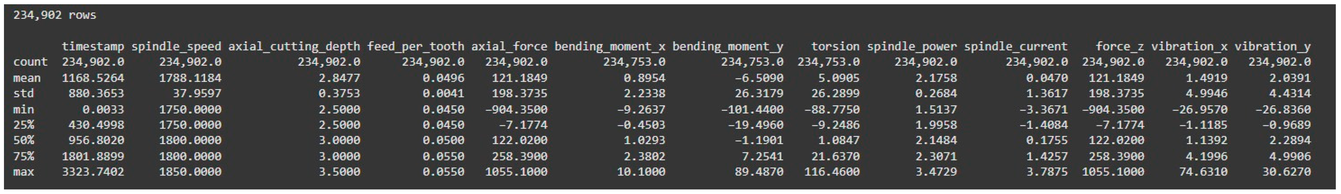
In the search for a suitable dataset for predicting insert wear in milling machines, several relevant public datasets are available. Among them, a dataset from the Katulu project’s GitHub repository [16] was selected as the origin of data for this research. A dataset called NUAA, extracted from NUAA Ideahouse, contains 24 variables and 234,902 rows of data from orthogonal milling experiments using solid carbide inserts and titanium parts (TC4).

Our research focuses on the NUAA dataset due to its greater number of variables, making it a more comprehensive option for a thorough analysis.

2.2. Method

To predict tool wear accurately, this study employed a systematic approach utilizing the NUAA dataset, which encompasses a wide range of inputs reflecting the complex relationships influencing tool wear. This comprehensive dataset facilitated the implementation of models specifically designed to learn and model nonlinear relationships between the input features and tool wear. The use of these models allowed us to capture intricate dynamics that would otherwise be overlooked, thus enhancing the accuracy of our predictions.

The analysis proceeded as follows:

• Data Selection and Preprocessing: The dataset was carefully curated and preprocessed to ensure consistency and relevance. This included cleaning the data, handling missing values, and normalizing features to prepare them for analysis.
• Pipeline Implementation: An AI pipeline consisting of ensemble models (Random Forest and Gradient Boost) and a Long Short-Term Memory network was used to compare the accuracy of tool wear prediction.
• Evaluation Metrics: The models were evaluated using appropriate metrics, such as the mean squared error (MSE), Mean Absolute Error (MAE), and Coefficient of Determination (R² Score), to assess their predictive accuracy and generalization capabilities.
• Visual Analysis: Different plots were generated to visually assess the distribution of predictions against actual values, providing insights into the best model’s performance and calibration. Additionally, a correlation matrix was implemented to explore relationships between variables within the dataset. This algorithm analyzed how different input features correlate with tool wear, aiming to uncover patterns that can inform predictive modeling and enhance our understanding of tool wear mechanisms.

2.3. Data Analysis and Pipeline Creation

An excerpt of the code developed specifically for this task can be found in Appendix A.

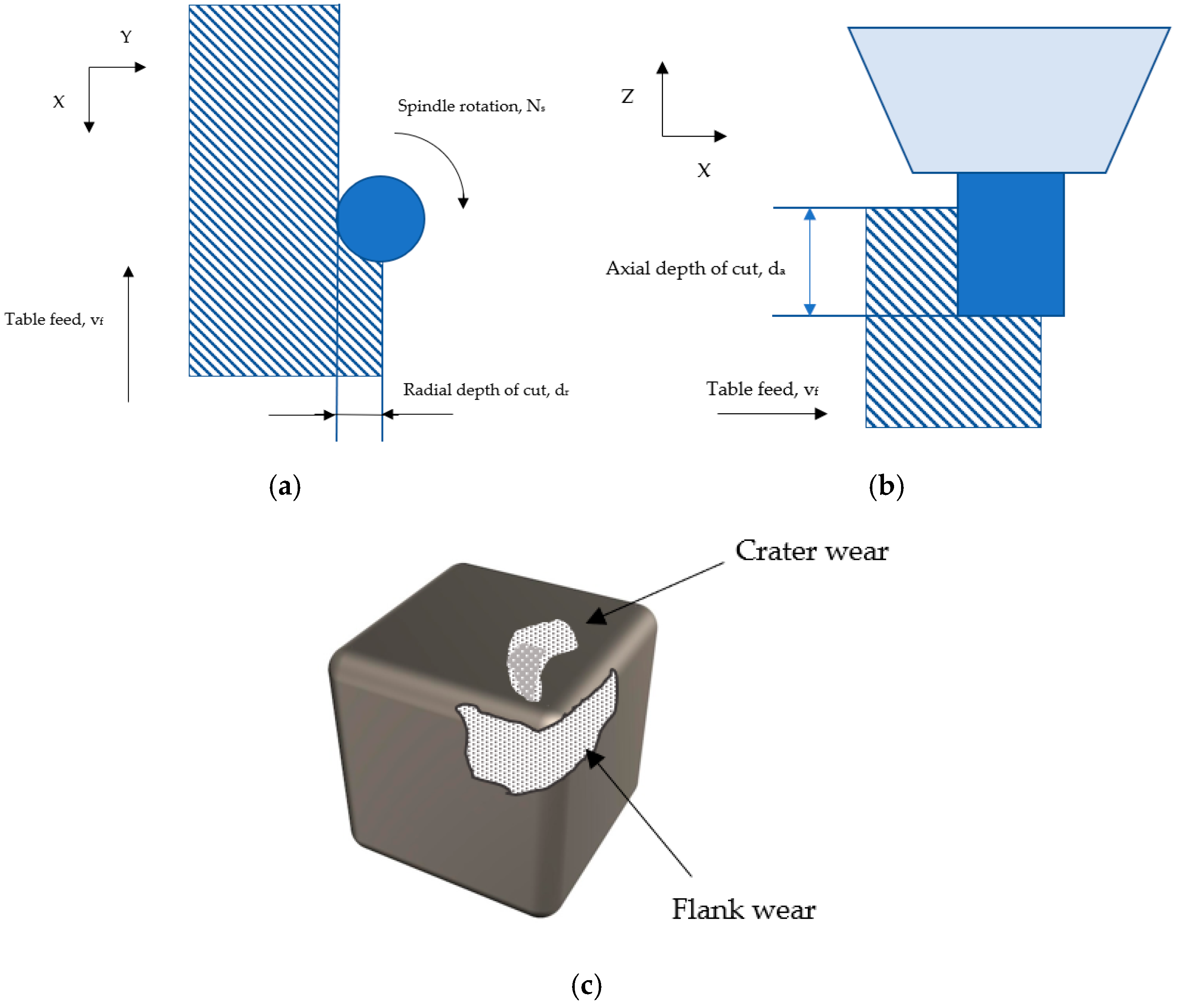
To begin the analysis, the NUAA dataset was loaded. Then, it was cleaned and reorganized by removing irrelevant columns and rearranging the remaining ones. With the data prepared, an initial exploration was conducted to understand the structure of the dataset. Figure 1 offers descriptive statistics that are reviewed to gain a better understanding of the data characteristics, Figure 2a,b remain as support images to help illustrate a generic milling operation diagram to clarify milling parameters [17,18,19], and Figure 2c illustrates the different types of tool wear, out of which flank wear is the focus of this article.

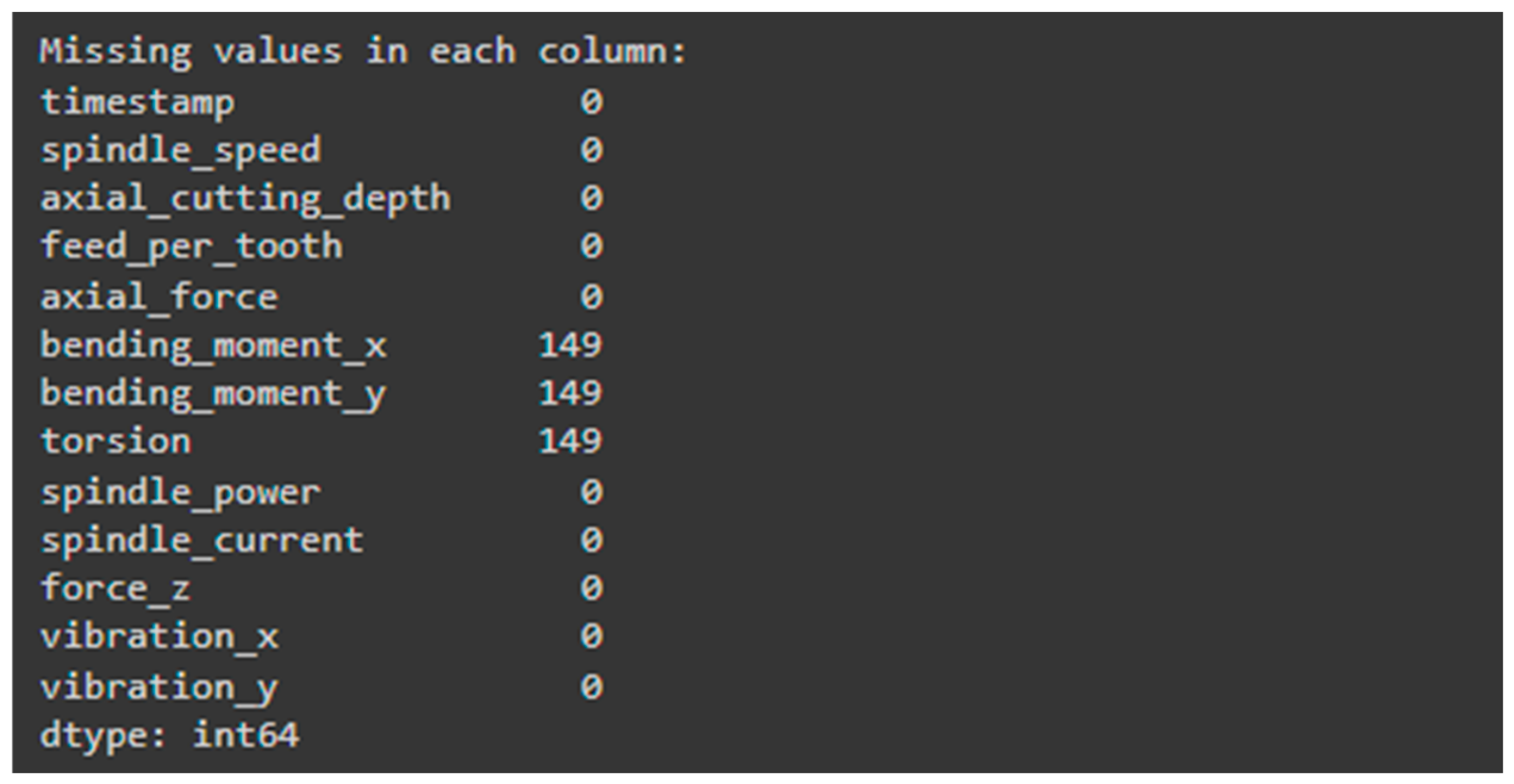
It can be seen (Figure 3) that out of the dataset, 149 rows are missing (null) values for bending moment x, bending moment y, and torsion, which could introduce errors during model training. To address this, we applied normalization to these rows instead of removing them.

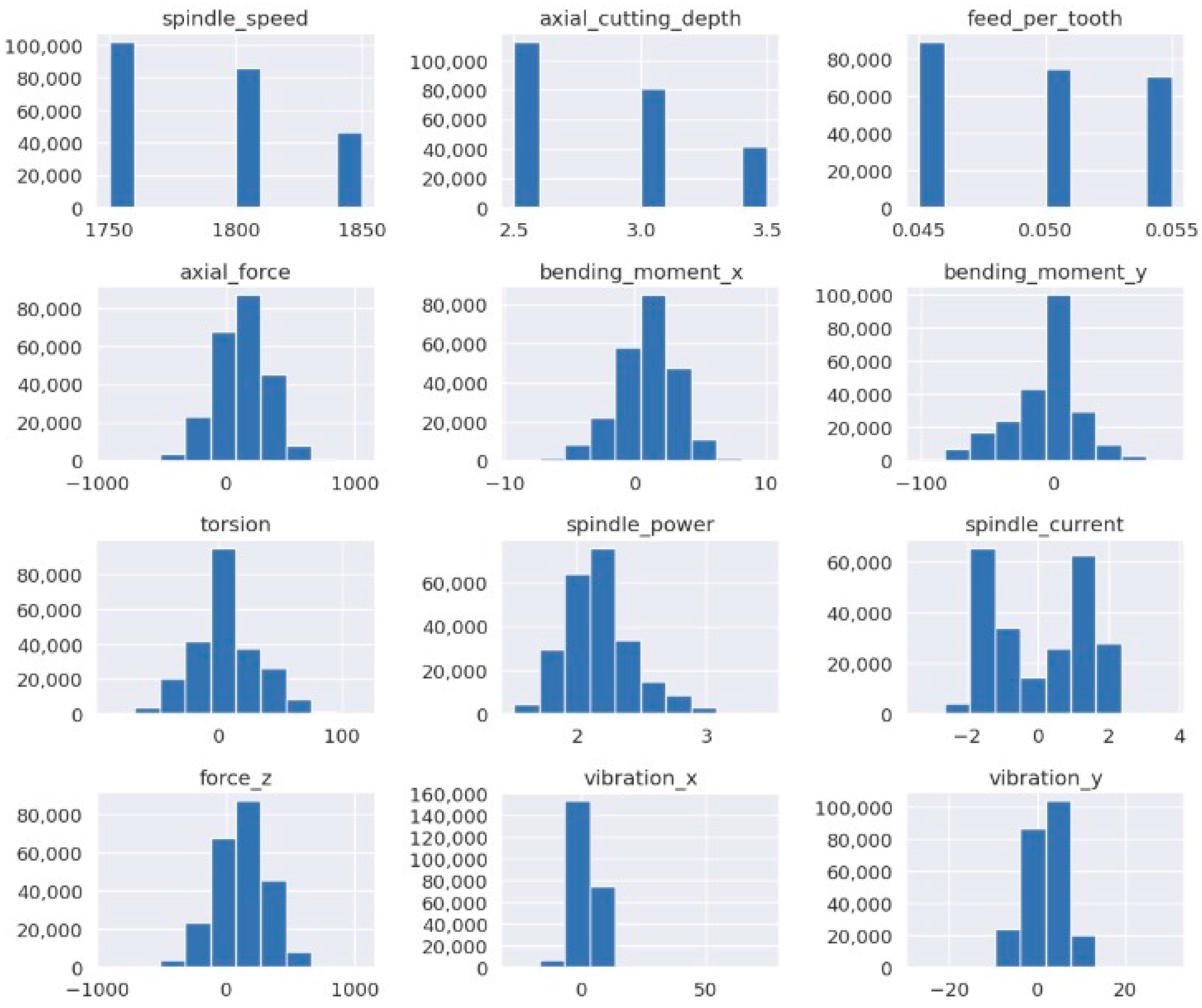
To gain a deeper understanding of the data, histograms were generated from the initial data exploration of the dataset, illustrating the distribution of the different characteristics. These graphs helped identify patterns and anomalies in the data (Figure 4). In the Y-axis, the total count of data is plotted, whereas the X-axis shows the data range of each variable in its respective units.

From the data distribution graphs, it can be observed that most values have a wide data range, except for the topmost three graphs, which have three columns, indicating that the owners of the dataset employed three constant values to obtain the others. Furthermore, while the Y-axis maintains consistent units across the graphs, the X-axis varies significantly. For example, in the feed per tooth graph, the values range from 0.04 to 0.06, whereas in the axial force graph, the range spans from −1000 to 1000. This disparity highlights the need for data normalization to ensure that the models can process the data effectively. It must be pointed out that those parameters can be negative, e.g., axial force can be physically negative because it represents a directional force along an axis. A negative axial force, such as −1000, indicates compression rather than tension, reflecting the direction in which the force is applied: positive forces align with the axis, while negative forces act in the opposite direction. In practical terms, a positive axial force pulls or stretches a structure, while a negative axial force pushes or compresses it.

To properly predict tool wear, a well-structured pipeline was leveraged to predict tool wear, employing a systematic approach to data preprocessing, model design, and validation. The process involved multiple steps, each critical to ensuring the models’ accuracy and robustness. The steps can be summarized as follows:

• Data Preparation and Preprocessing.

First, the dataset was processed to handle any potential inconsistencies. Any non-numeric values in the dataset were coerced into a numerical format, and any rows containing missing values were removed to ensure that the models only trained on clean and complete data, reducing the risk of errors during training.

Next, the dataset was split into features and the target variable. The features, which were various characteristics of the cutting tools, formed the input to the models, while the target variable was the tool wear, which the models were supposed to predict. Then, the data were divided into training and testing sets using an 80/20 ratio, meaning 80% of the data was used to train the models, while the remaining 20% was reserved for testing their performance.

Because different features can have different ranges and units, scaling was necessary. A standard scaler was used to normalize the feature values. The scaler transformed the data such that each feature had a mean of 0 and a standard deviation of 1. This step is critical for neural networks because it ensures that all inputs are treated equally by the model, helping to prevent any one feature from dominating the learning process.

2.

Pipeline and Model Architecture Designs.

A comprehensive Machine Learning pipeline was developed incorporating ensemble models and an LSTM (Long Short-Term Memory) network to enhance the accuracy of tool wear prediction. The pipeline consisted of data preprocessing, ensemble modeling, temporal modeling with LSTM, and model evaluation.

Two ensemble models—Random Forest and Gradient Boosting—were employed to leverage the strength of multiple decision trees.

• Random Forest: Consisting of 100 decision trees, the model uses multiple random samples and averages predictions to reduce variance.
• Gradient Boosting: This model sequentially improves predictions by focusing on areas where previous models performed poorly, capturing complex data patterns.

Additionally, to capture temporal dependencies in the data, an LSTM network was implemented to model time-series behavior, which is useful for sequential dependencies like tool wear progression. A time window of 5 was set, allowing the model to predict tool wear based on the previous five time steps.

• LSTM Architecture: The LSTM layer, containing 64 units, captures sequential data patterns, while a dropout layer with a 20% rate helps prevent overfitting. The model’s output layer consists of a single neuron, reflecting the regression task.
• Early Stopping: To avoid overfitting, early stopping was implemented, halting training once validation loss stopped improving.

3.

Model Validation with Cross-Validation.

To evaluate the models’ generalization performance, K-Fold cross-validation with five splits was used. This approach divided the training data into five equally sized subsets. The models were iteratively trained on four of these subsets and validated on the remaining one, cycling through each fold to ensure the models were tested on all portions of the data. By doing so, every data point in the dataset was used for both training and validation, providing a comprehensive assessment of the model’s performance. This method reduces the variability that might result from relying on a single train–test split and ensures a more reliable estimation of the model’s predictive capabilities.

The results from the cross-validation process were calculated using the MSE, which measures how well the models fit the training data. The average MSE across the folds was reported, along with the standard deviation, which gave an idea of how consistent the models’ performances were across different subsets of the data.

4.

Early Stopping Mechanism.

To prevent overfitting, an early stopping mechanism was implemented during training. Early stopping monitors the models’ losses during training and halts the process if the losses fail to improve for a set number of epochs (in this case, 10). Additionally, the best weights of the models are restored once training stops, ensuring the best possible model is used for predictions.

5.

Model Testing and Final Evaluation.

Once the models were trained and cross-validated, they were tested on the unseen test set. The test data were scaled using the same scaler fitted on the training data to ensure consistency. The model’s performances on the test set were evaluated using the MSE, which provided an estimate of how well the models generalize to new, unseen data. This final MSE score gave a clear indication of the model’s predictive accuracy.

3. Results

From the cross-validation training, the following cross-validated MSE values were obtained for the Random Forest, Gradient Boosting, and LSTE models, respectively: 2.05 × 10⁻⁸, 8.14 × 10⁻⁵, and 5.88 × 10⁻³ with a standard deviation of 2.18 × 10⁻⁸, 4.56 × 10⁻⁶, and 5.22 × 10⁻⁵. Each fold of the training ran for a varying number of epochs, a variability that shows that early stopping occurred at different times across the folds to avoid overfitting.

After training on the complete training data, the following MSE values were obtained for the test set predictions, in the same order aforementioned: 4.7 × 10⁻⁹, 7.4 × 10⁻⁵, and 5.6 × 10⁻³.

The Gradient Boosting model was chosen as the model to be implemented due to its ability to capture complex, nonlinear relationships and its adaptability to smaller datasets compared to Random Forest and LSTM. During cross-validation, Gradient Boosting demonstrated competitive performance, with its mean squared error being higher than Random Forest but still reasonable. Its ability to iteratively refine errors through its sequential learning process makes it more suited to datasets with intricate patterns. Furthermore, Gradient Boosting’s stepwise construction of decision trees provides valuable insights into feature importance, improving the interpretability of its predictions. Although its standard deviation was higher than that of Random Forest, the model still exhibited strong generalization on the test set. This combination of performance, interpretability, and adaptability, particularly when hyperparameters are finely tuned, makes Gradient Boosting a robust choice. As such, it will be referred to as “the model” throughout the remainder of this study, representing the optimal approach for predictive tool wear analysis.

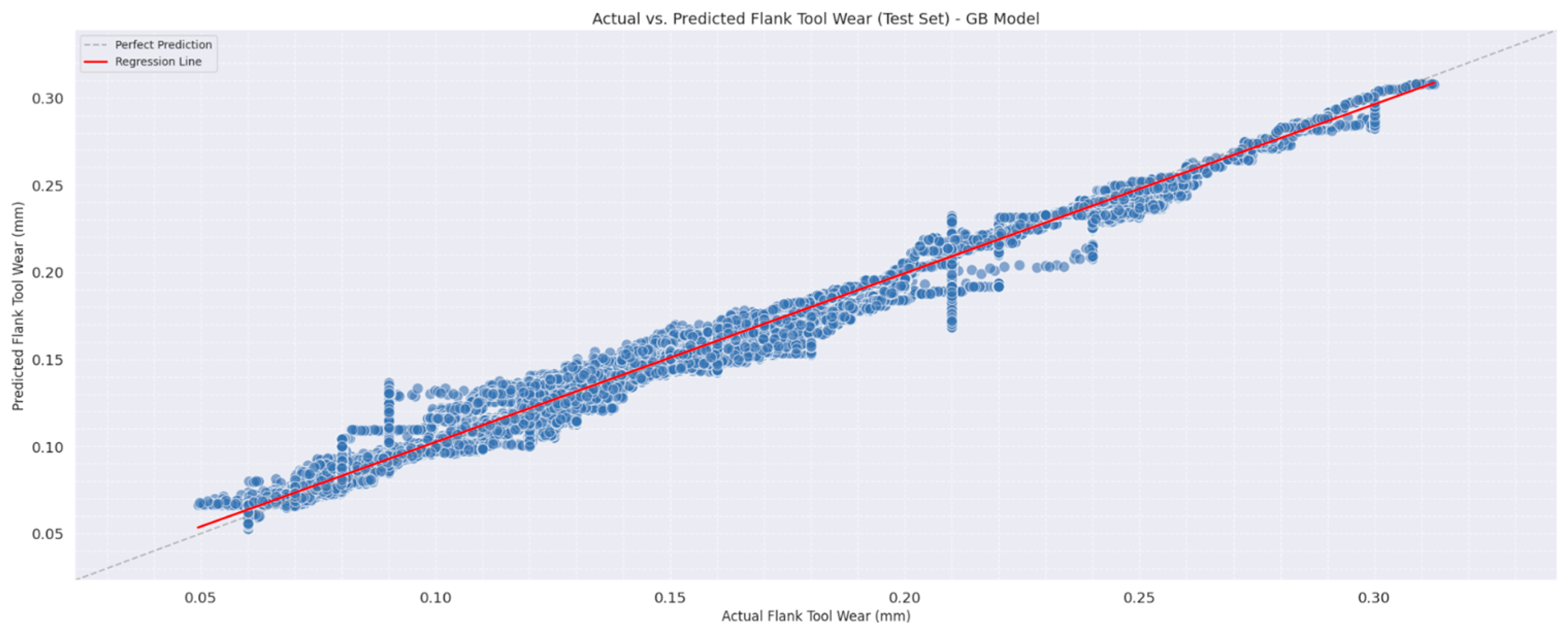
The first plot (Figure 5) compares actual and predicted tool wear values. This scatter plot, with a regression line, shows how closely the model’s predictions align with the true values. Each point represents a prediction, and the red line represents perfect predictions, where actual equals predicted. Ideally, the points should be as close to this line as possible. In this case, the points generally follow the regression line, indicating a strong positive correlation between the actual and predicted values. However, the deviations observed at medium tool wear levels, often referred to as outliers, suggest that the model faces some difficulty in accurately predicting certain values. This does not necessarily indicate poor model performance. It is often a positive sign that the model is not overly precise, as perfect accuracy could imply overfitting. By not being excessively precise, the model demonstrates a level of flexibility, suggesting it will generalize better to new, unseen data. Balancing prediction accuracy with generalization is key to building a robust and reliable model.

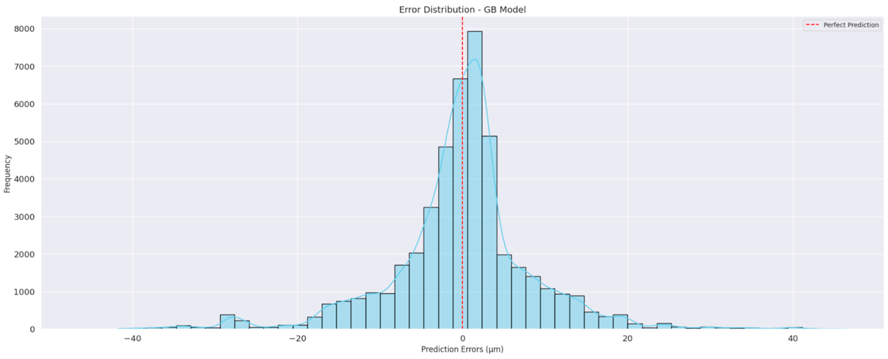
The second plot (Figure 6) visualizes the error distribution, showing the difference between the actual and predicted values. The distribution should ideally be centered around zero, indicating that the model’s errors are balanced and not consistently over- or underestimating tool wear. The histogram shows a relatively symmetric error distribution around zero, with a narrow spread. This suggests that most of the model’s predictions are close to the actual values, with a few larger errors appearing in the tails of the distribution.

The third plot (Figure 7) compares the overall distribution of the actual and predicted tool wear values using density plots. The blue curve represents the actual tool wear, while the orange curve represents the predicted values. The degree of overlap between these curves shows how well the model captures the general pattern of the data. Here, the predicted distribution follows the actual distribution quite well, especially for moderate tool wear values, although the model seems to underperform in predicting extreme tool wear, which leads to a slight mismatch at the higher values.

The model’s performance on the test set was evaluated using three metrics: MAE, MSE, and R² Score. MAE measures the average magnitude of the errors between predicted and actual values, indicating how much the predictions deviate from the actual values on average. MSE squares the errors, giving more weight to larger errors, and is useful for identifying significant prediction discrepancies. The R² score indicates how well the model explains the variance in the target variable. An R² score of 1 means the model perfectly predicts the target, whereas a value closer to 0 means the model performs no better than simply predicting the mean of the target variable. An acceptable R² for regression cases generally falls between 0.5 and 0.99, according to Ozili [20], with a strong R² score being above 0.90.

After predicting the tool wear values with our test set, the following parameters were obtained:

• MAE: 5.7821 × 10⁻³ mm. This means, on average, the model’s predictions are off by about that many units of tool wear.
• MSE: 7.4263 × 10⁻⁵ mm. The low value indicates that the model makes a few large errors.
• R² score: 0.9857. This suggests that the model explains 98.57% of the variance in the tool wear values.

3.1. Correlation Matrix

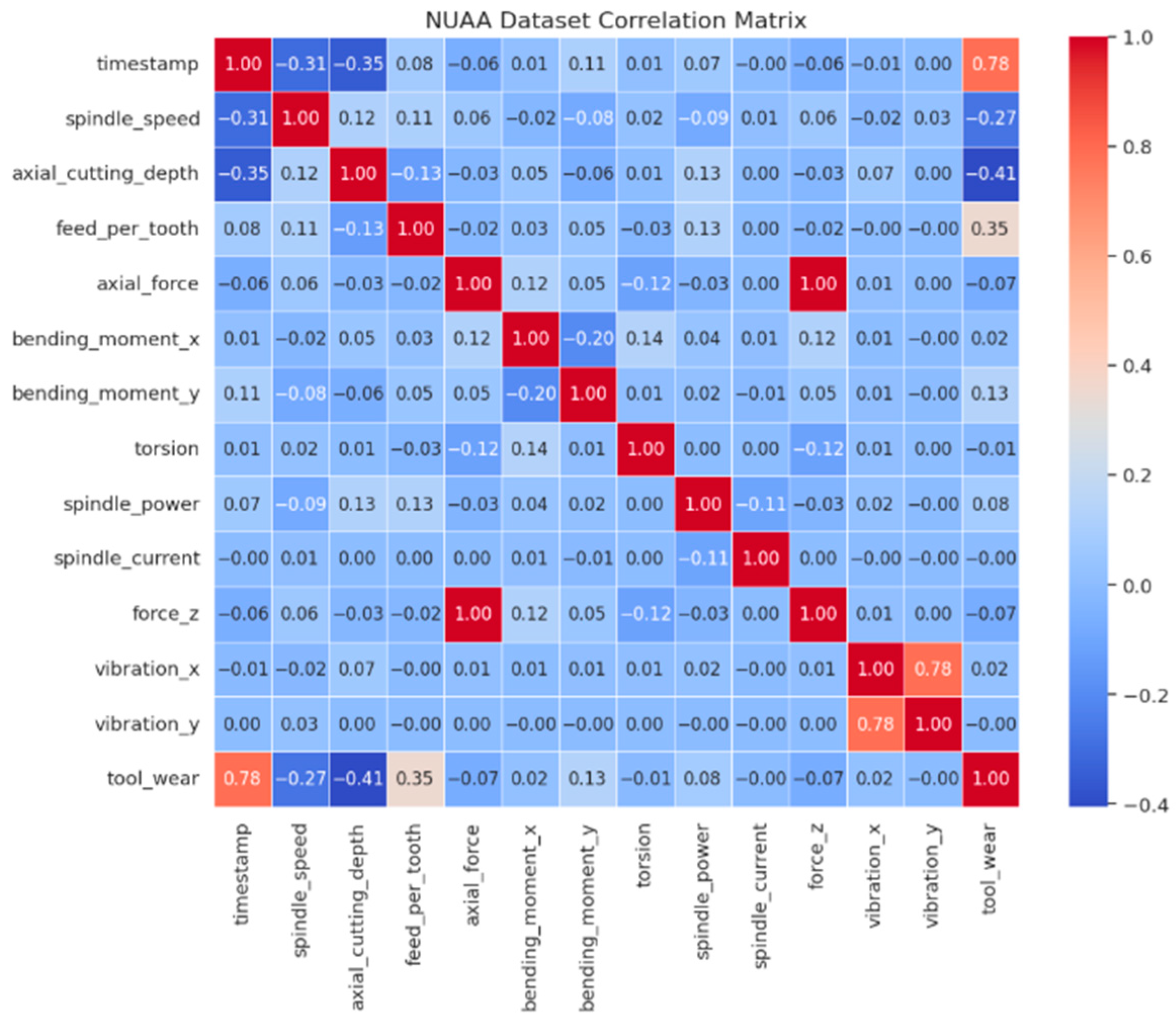
In the analysis of complex data, especially when dealing with multiple variables, it is important to identify patterns and relationships that may influence the desired outcome. In the case of this research, there is an interest in seeing how different variables affect tool wear. To facilitate this task, a correlation matrix can be used to quantify the linear relationship between each pair of variables in the dataset. This allows for the evaluation of how variables such as axial force, spindle speed, and vibrations correlate with tool wear. Each value in the matrix represents the Pearson correlation coefficient, which ranges from −1 to 1; values close to these limits indicate strong positive or negative correlations, respectively, while values close to 0 suggest a weak relationship. By visualizing the matrix (Figure 8) with a heat map, significant relationships and emerging patterns can be quickly identified, allowing the analysis and modeling to focus on the variables that have the greatest impact on wear [21] or even consider others that may have been overlooked.

When analyzing the correlation matrix of the NUAA dataset (Figure 8), relationships emerge that align with the initial expectations of this study. In particular, the last row highlights a strong positive correlation between wear and time, which is consistent with the notion that wear tends to increase as time passes. Moreover, a moderate negative correlation is identified between wear and both cutting depth and spindle speed, suggesting that increasing these variables significantly reduces wear. The lack of data could imply that this might be due to factors such as energy dissipation or the distribution of stresses during the cutting process, though it could also be attributed to a decrease in cutting depth. A strong direct relationship is observed between vibrations on the X-axis and those on the Y-axis, as well as a total correlation between axial force and force Z, probably indicating that they have the same data with different variable names. Lastly, the feed per tooth shows a positive correlation with wear, although it is not very high, thus establishing that as the feed per tooth increases, wear also increases.

3.2. Remaining Useful Life (RUL) Prediction

RUL is a critical metric in predictive maintenance and reliability analysis, serving to estimate the time remaining before a component or system experiences failure or necessitates maintenance. In this analysis, predictive models are employed to forecast the future wear of a tool based on various input characteristics, thus indirectly calculating the RUL by predicting the expected wear that will occur over time. Rather than determining the RUL directly, the focus is on predicting future tool wear, which can effectively serve as a proxy for RUL if wear is recognized as an indicator of the time until failure.

To facilitate this analysis, the NUAA dataset is utilized due to its rich array of variables, which are essential for accurate predictions. In this approach, fixed values are applied, and a pre-trained Gradient Boosting model will assesses the tool’s wear, ultimately allowing for the determination of the remaining useful life of the tool. This method harnesses the dataset’s comprehensive features to enhance the reliability and accuracy of RUL predictions.

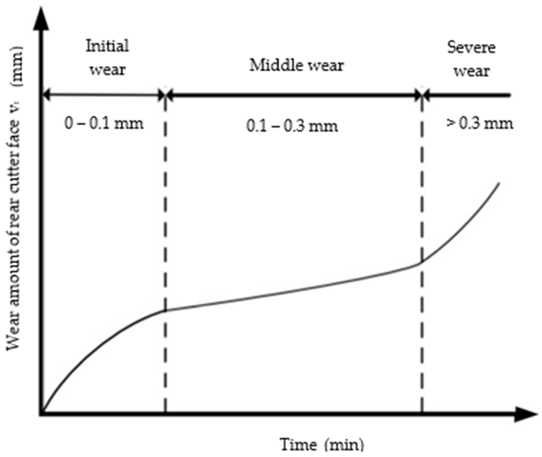
The graph presented in Figure 9 closely resembles the graph generated from Taylor’s equation [22], with the Y-axis indicating the wear bandwidth as a function of time. It reveals three distinct zones, each representing specific wear levels and their corresponding severity for the cutting tool. The dataset demonstrates a wear range spanning from 0.049 mm to 0.31 mm, aligning well with the graph’s scale and enabling the extraction of meaningful conclusions and physical interpretations from the mathematical results produced by the recently trained Gradient Boosting model.

From the analysis of the correlation matrix, two parameters that exhibit a relatively somewhat strong relationship with tool wear are identified: spindle speed and feed per tooth. These parameters are input into the Gradient Boosting model, using mean values for the other variables, to calculate the time required to achieve the target wear levels. This analysis facilitates an approximate determination of the time it will take for the cutting tool to reach the specified wear thresholds corresponding to the three zones identified in the preceding graph (0.1 mm, 0.2 mm, and 0.3 mm).

Importantly, even with variations in parameters, the predictive model can be continuously updated with real-time data, allowing for adjustments to the expected time. Consequently, operators will maintain precise awareness of when the cutting tool is projected to enter the dangerous wear zone, with a recommendation to replace the insert when wear values fall between 0.25 mm and 0.3 mm to ensure a high-quality finish on the machined product.

While the NUAA dataset is derived from a specific insert and tool material, the findings can readily be extrapolated to other inserts if the materials are comparable. For instance, consider the insert model 345R-13T5E-ML S30T (Sandvik Coromant, Sandviken, Sweden) [23], which is coated with titanium and designed for use with solid carbide parts, consistent with the materials specified in the chosen dataset. From its manufacturer’s datasheet, the following values are obtained:

• Feed per Tooth (f_z): 0.11 mm/rev; range: 0.07–0.20 mm/rev.
• Cutting Speed (v_c): 140 m/min; range: 120–155 m/min.

The value for f_z is directly incorporated into the code as a value. Subsequently, the cutting speed formula is applied, assuming a DC_ap (cutting diameter at the depth of cut) of 0.03 m to calculate the spindle speed, which, after rounding, yields a result of 1485 rpm. Upon inputting these parameters into the trained Gradient Boosting model, the following times are obtained:

• For a wear value of 0.1 mm: Time: 0:06:40.
• For a wear value of 0.2 mm: Time: 0:13:20.
• For a wear value of 0.3 mm: Time: 0:48:20.

To interpret these results, it is of great importance to reference Taylor’s equation and analyze the preceding graph. In the initial phase (initial wear), which spans from 0 to 0.1 mm, the wear exhibits a nonlinear function, indicating rapid degradation based on the input parameters and the insert material. This phase is characterized by the tool’s settling process, during which the cutting insert adjusts to the material being machined, effectively eliminating surface irregularities and micro-defects. Physically, this phase may reveal visible wear at the tool’s cutting edges, a slight increase in surface roughness, and noticeable changes in cutting sounds and forces.

The second phase (middle wear), occurring within the wear range of 0.2 to 0.3 mm, presents a more stable and predictable wear rate. By this point, the insert has transitioned beyond the settling stage, resulting in more uniform wear. The relationship between time and wear becomes increasingly linear, enabling interpolation to predict wear at intermediate points, such as 0.25 mm. This threshold is critical, as it is the point at which tool replacement should be considered to prevent issues like diminished cut quality, increased cutting forces, and vibrations that could adversely impact the final product. During this phase, the tool’s edge begins to round off more significantly, and while the cut quality starts to decline, it remains within acceptable limits.

As wear approaches 0.3 mm, operators enter a critical zone where wear accelerates again, marking the beginning of the third phase where severe wear occurs. At this stage, it is imperative to replace the tool, as prolonging its use could result in severe failures, such as tool breakage or damage to the workpiece. Operators may experience a marked increase in cutting forces, elevated temperatures, and alterations in sound, all indicating that the tool is under considerable stress. The quality of the machined surface may deteriorate rapidly, displaying visible signs of wear such as rough edges or even deformation of the workpiece. This phase is characterized by flank wear and potentially abrasive wear, making it essential not to exceed the recommended wear limits for inserts (between 0.25 and 0.3 mm).

4. Discussion

The objective of this investigation is to assess the tool wear of milling inserts through Machine Learning algorithms and data analysis. Numerous studies have explored the application of artificial intelligence techniques for monitoring wear in milling machines. According to a systematic review by Munaro et al. [6], there has been a notable increase in AI-related publications focused on machining operations since 2010, particularly concerning tool wear and the remaining service life of cutting tools. These studies highlight various Machine Learning algorithms, including artificial neural networks (ANNs), Fuzzy Logic algorithms (FLs), support vector machines (SVMs), decision trees and Random Forests (RFs), Bayesian networks (BNs), and convolutional neural networks (CNNs).

By turn, in their research, Kim et al. [24] proposed an innovative method for predicting tool wear using deep CNNs, known for their ability to learn hierarchical data representations through multiple convolutional layers. This CNN model architecture utilizes multi-scale convolutional kernels, which are crucial for capturing features of varying sizes in the input data. This capability is particularly relevant for predicting tool wear in machining processes, as it enables the model to recognize patterns across different scales, thus enhancing prediction accuracy. Additionally, Bayesian learning is introduced, incorporating principles of probability theory to manage uncertainty in predictions. By transforming the CNN model into a probabilistic framework, it becomes possible to estimate the uncertainty associated with wear predictions, which is vital for industrial applications. The integration of Bayesian learning allows the model to provide not only point predictions but also confidence estimates, making it especially valuable in processes like titanium alloy milling, where conditions can fluctuate and tool wear is unpredictable. While this model demonstrated a low mean square error and an R² score exceeding 0.9, our model achieved an R² value of 0.9857, surpassing the performance of the most advanced models, such as the Bayesian DMSCNN, which attained an average R² of 0.96. Notably, our model accomplished this with fewer cross-validation folds (5 vs. 10), fewer available data, and a broader range of variables, resulting in a very low mean MAE and MSE. This indicates that the model not only maintains competitive predictive accuracy but also demonstrates robust performance under challenging conditions.

Meng et al. [25] proposed an advanced approach for feature selection in predictive models by using singular value decomposition (SVD) combined with a voting scheme. In their study, the authors applied this technique to reduce the dimensionality of the dataset and then employed a voting scheme to select the most relevant features. This approach was complemented by three feature classification methods: Random Forest, Principal Component Analysis followed by Principal Component Regression (PCA + PCR), and Pearson Correlation Coefficient (PCC). The combination of SVD with PCA + PCR proved particularly effective, yielding the lowest mean square error [25]. This suggests that integrating advanced decomposition and feature selection techniques can significantly enhance the accuracy of predictive models by optimizing the relevance of the considered variables. Although our dataset was thoroughly cleaned and the features were handpicked to train the Gradient Boosting model, a careful examination of variables related to tool wear was conducted, adopting the findings of authors like Meng et al. Their research highlighted the significance of specific features in predicting tool wear, which can be corroborated by their results through a correlation matrix. This matrix effectively validated their hypothesis, demonstrating that the selected features have meaningful relationships with tool wear, which further strengthened the predictive capability of our model.

For its part, Random Forest regression effectively combines filter and wrapper methods to select features, providing a detailed analysis of each feature’s importance in the model [26]. This not only evaluates the relevance of the features but also organizes them in descending order according to their impact on reducing model impurity. Feature selection in RFR utilizes a low-variance filter, Spearman correlation, and Random Forest regression [25]. The low-variance filter eliminates features with minimal variability, while Spearman correlation measures the monotonic relationship between variables, and RF regression analyzes how each feature contributes to the overall accuracy of the model. This allows the algorithm to manage complex data and provide a detailed assessment of each parameter’s importance in the model’s performance, thereby ensuring greater accuracy and generalization [25,26,27,28]. While Meng et al. achieved significant improvements with their methods, the approach presented in this article simplifies the selection process by training a Gradient Boosting model with all relevant variables that have a strong correlation with tool wear—as seen in the correlation matrix—while still yielding competitive performance.

Compared to neural network models, SVMs often exhibit superior generalization abilities, particularly when training data are limited. Gomes et al. [29] introduced a novel method for monitoring tool wear in the micro-milling process using an SVM artificial intelligence model combined with vibration and sound signals. This approach addresses the limitations of traditional methods by integrating multiple types of sensory data, significantly improving accuracy in detecting tool wear. The incorporation of vibration and sound signals resulted in a richer dataset, enabling the SVM model to discern patterns that may be obscured with a single type of signal. Building on this concept, Niu et al. [30] developed a multi-stage SVM to identify tool wear based on selected features, allowing for more precise identification by processing features through multiple analytical stages. This method proved effective in managing the complexity of and variability in wear data. However, the performance of the SVM model is heavily dependent on the selection of penalty factors and Kernel function parameters. In their study, the maximum prediction accuracies for BP neural networks, Bayesian networks, and SVM were 83%, 75%, and 72%, respectively—impressive performances, yet not the most precise. In contrast, our model was trained with the same (and more) variables—vibrations, for instance—and achieved a superior “accuracy” by obtaining lower MSE and MAE scores, thus improving the predictive capabilities of previous models.

Furthermore, the Gradient Boosting model of this study had an impressive performance given its relative simplicity, as shown by the obtained metrics; hence, there is no immediate need to enhance the model for this task. However, should the decision be made to pursue further improvements, several strategies could be considered to potentially enhance its efficacy. While the proposed models demonstrate promising performance, it is important to acknowledge the limitations associated with the dataset size. The training dataset, although robust, may not fully capture the wide range of variations in machining conditions and tool wear patterns encountered in real-world industrial settings. To mitigate this limitation, we employed K-Fold cross-validation with five splits to rigorously evaluate the generalization capacity of the models. While our current approach used standard K-Fold cross-validation, future research could benefit from implementing stratified K-Fold cross-validation to ensure a more consistent representation of tool wear characteristics across all folds. Future studies should also prioritize expanding the dataset by incorporating additional data points or generating new experimental data to further enhance the models’ robustness and applicability to diverse scenarios.

In addition to the existing dataset limitations, future studies should prioritize the integration of environmental variables into the predictive modeling process. Factors such as temperature and humidity, which can significantly influence tool wear behavior, are not accounted for in the current dataset. To address this, we suggest the deployment of sensors capable of measuring these parameters during machining processes. The data collected from such sensors could serve as additional inputs for the predictive models, enabling them to capture a more nuanced understanding of the tool wear mechanisms under varying environmental conditions. Incorporating this layer of information would not only improve model precision but also enhance its applicability to real-world industrial settings where environmental fluctuations are prevalent.

Another limitation of this study lies in the reliance on pre-collected data from public datasets, which, while convenient and robust, may introduce inherent biases or omit key variables relevant to tool wear prediction. Factors such as variations in machining setups, operational conditions, or even data collection methods can affect the generalizability of the findings. To address this, future research should prioritize the creation of tailored experimental datasets that capture a broader range of tool wear scenarios, incorporating diverse materials, machining environments, and operating parameters. Additionally, leveraging advanced data preprocessing techniques, such as bias detection and correction methods, can help mitigate the influence of such limitations, ensuring that predictive models are both accurate and suited for various industrial applications.

Tool wear is a complex, dynamic process that is influenced by many variables, which are not only interconnected but also fluctuate over time, complicating the task of accurately modeling wear patterns. Current models, while valuable, are often limited in their ability to fully capture these dynamic interactions. As a result, future research should explore the application of advanced methodologies such as deep neural networks, which excel at modeling nonlinear and high-dimensional relationships. Furthermore, reinforcement learning offers the potential to continuously adapt to evolving wear conditions, providing a dynamic framework for more accurate predictions. These advanced approaches, coupled with transfer learning, could enable models to generalize more effectively across diverse machining environments, improving their applicability to real-world industrial settings.

Future research could also consider the development of hybrid or ensemble models as well that combine the strengths of different Machine Learning approaches, such as Gradient Boosting and LSTM. These models could harness the complementary benefits of ensemble techniques and sequential learning to improve predictive accuracy and robustness. Additionally, integrating these predictive models into existing manufacturing execution systems would facilitate their practical implementation in industrial settings. Such integration could enable real-time tool wear monitoring and adaptive decision-making.

Moreover, evaluating the model’s performance on alternative test sets can yield valuable insights into its reliability across different scenarios. This practice is essential to ensure that the model is not overly fitted to a specific dataset, thus providing a more comprehensive understanding of its predictive performance.

Additionally, implementing a grid search for hyperparameter optimization could facilitate the identification of optimal model parameters. This methodical exploration of parameter combinations allows for fine-tuning, which can lead to significant improvements in accuracy and predictive capability. By rigorously refining the model in this manner, it can be ensured that it remains both robust and adaptable to diverse datasets and operational contexts. Such efforts would ultimately bolster the model’s applicability and effectiveness in real-world applications.

While the NUAA dataset is based on solid carbide inserts and titanium parts, we have further analyzed the extent to which the proposed methodology can be applied to other materials and tools. By considering the fundamental properties that influence tool wear (e.g., hardness, thermal conductivity, and cutting force resistance), we have identified commonalities between the materials in the dataset and other industrial materials like high-speed steel and certain ceramic inserts. Future studies could validate these observations through experimental testing with diverse materials to confirm the robustness of the proposed models.

5. Conclusions

This research provides a comprehensive analysis of tool wear in milling machines, focusing on the precise prediction of remaining tool life through the implementation of artificial intelligence algorithms. Throughout the development, the purpose of milling machines and their cutting tools, particularly milling inserts, is thoroughly examined, highlighting the advantages they offer over solid tools. The phenomenon of tool wear is explained in detail, emphasizing its direct impact on product quality and process efficiency, culminating in a direct application of Machine Learning models to accurately predict wear in insert blades.

One of the key achievements of this work is the improvement in the accuracy of predictive models compared to what has been previously reported in the literature. The use of a simple Gradient Boosting model enables a more accurate prediction of wear compared to other models like neural networks and SVMs and is relatively close to that of more deep learning models that require extensive tuning and large datasets. Furthermore, it overcomes limitations observed in prior studies, where wear predictions relied on overly complex methods and a greater number of variables, obtaining an even lower R² score than our model.

Additionally, a proper relationship between variables is established, explaining the correlation between the different variables involved. Specifically, this work demonstrates that AI models, when properly tuned (cross-validation, train–test splitting, and regularization) and applied, can effectively capture the complex relationships among the involved variables, thereby enhancing the accuracy and reliability of their predictions.

The proposed methodology not only addresses the challenges of tool wear prediction but also provides valuable insights for future research in the field of machining. By employing a data-driven approach that integrates advanced AI techniques, this study lays the groundwork for developing more robust predictive models that can adapt to various machining conditions and contribute to solving potential limitations that could appear in these processes.

Moreover, the incorporation of uncertainty awareness in predictions paves the way for more informed decision-making processes within manufacturing environments. As industries increasingly shift towards smart manufacturing, the findings of this research can significantly enhance operational efficiency and product quality, ultimately leading to improved customer satisfaction as products will be affected by cost reduction.

The methodology employed in applying AI could be transferable to other manufacturing processes by adapting the algorithms.

This study underscores the importance of harnessing AI algorithms in machining processes to achieve reliable tool wear predictions. Future work could explore the applicability of these models in different manufacturing contexts and investigate the integration of real-time monitoring systems to further enhance predictive accuracy and reliability.

Finally, as previously noted, wear is a complex phenomenon influenced by numerous factors, including forces, vibrations, temperature, and material properties. While this model offers a reliable approximation, it could be significantly enhanced by integrating more relevant parameters related to the process. Using sensors and other techniques to collect real-time data thereby will improve input accuracy and ultimately enhance output predictions with artificial intelligence techniques.