Article

Breast Histopathological Image Classification Based on Auto-Encoder Reconstructed Domain Adaptation

School of Microelectronics and Communication Engineering, Chongqing University, Chongqing 400044, China
*
Author to whom correspondence should be addressed.
Appl. Sci. 2024, 14(24), 11802; https://doi.org/10.3390/app142411802
Submission received: 12 November 2024 / Revised: 13 December 2024 / Accepted: 15 December 2024 / Published: 17 December 2024

Abstract

:
As an effective computer-aided diagnostic tool, deep learning has been successfully applied to the classification of breast histopathological images. However, the performance of the deep model is data-driven, and it is difficult to obtain satisfied results when the number of histopathological images is small and labelling histopathological images is difficult. Moreover, in traditional deep learning methods, the representation of features is monotonous, which leads to the limitation of the classification performance of the model. This study proposes an auto-encoder reconstructed semi-supervised domain adaptation for a breast histopathological image classification algorithm. First, the model was pre-trained and transferred to extract high-level features of the sample images. Then, the encoding and decoding parts of the auto-encoder were used to reconstruct the feature representation learning and the sample feature reconstruction learning, respectively. This ensured that the useful information for the classification was purified and retained. At the same time, the domain discriminator was used to confuse the source and target domain features to enhance the learning ability of the model. Finally, the distribution difference of features at different depths of the auto-encoder was measured to minimize the discrepancy of feature distribution between domains, so as to complete the classification of histopathological images. Compared to the results of the comparative and ablation algorithms from the BreakHis to SNL datasets, the proposed method achieved the best results in terms of F1 score (93.40%), accuracy (95.24%), sensitivity (94.66%), and specificity (95.56%). The experimental results demonstrate that the proposed method achieves a remarkable classification performance.

1. Introduction

Breast cancer is one of the most serious diseases threatening women’s health. Accurate diagnosis is crucial for patient survival. Among various diagnostic methods, clinical histopathological diagnosis serves as the gold standard for breast cancer detection. However, manual detection is not only time-consuming and labor-intensive, but also requires the experience of examiners. As an effective computer-aided diagnostic (CAD) tool, deep learning has been extensively applied to breast histopathological image classification tasks [1,2,3]. The key to address the contradiction between high detection demand and limited examiners lies in establishing efficient deep learning models.
Developing stable deep learning diagnostic algorithms faces two challenges. Firstly, deep models require a large amount of labeled data; otherwise, they may suffer from insufficient generalization ability and overfitting [4,5]. Labeling histopathological images requires an experienced pathologist, and the labeling process is extremely time-consuming. Developing deep models based on limited labeled data poses a significant challenge. Additionally, low-level features such as texture and shape are very useful for histopathological image classification. Hence, efficiently fusing multi-level features represents another challenge.
Our motivation is to address the two challenges faced by histopathological image classification models. A semi-supervised domain adaptation (DA) method is proposed to address the labelled data shortage issue, and on the other hand, an auto-encoder is applied to reconstruct image features, refining and preserving useful information for classification. We aim to enhance the performance of domain adaptation algorithms by reconstructing sample features.
This paper introduces an auto-encoder reconstructed semi-supervised domain adaptation algorithm for breast histopathological image classification. This algorithm employs a deep transfer network to obtain multi-level features of histopathological images. The samples from two domains are confused using similarity loss and domain discriminators in order to blur the boundaries between domains. A lightweight auto-encoder is created for feature reconstruction. The encoder not only compresses the extracted features and mines representation embedding, but also learns domain-invariant information. Additionally, the decoder uses reconstruction loss as a constraint for feature reconstruction, prompting the model to learn representations for classification tasks. During the feature extraction and reconstruction process, the difference in feature distribution between the source and target domains is measured multiple times to enhance the discriminative accuracy of the sample classifier.
The rest of this paper is structured as follows: In Section 2, we will specifically introduce previous related research works and the differences from the proposed method. In Section 3, the proposed method is presented in detail. In Section 4, the comparative experiments and ablation experiments are presented and analyzed. Finally, we conclude the paper in Section 5 and offer outlooks for future work.

2. Related Work

Deep learning, especially Convolutional Neural Network (CNN)-based CAD algorithms, has been extensively applied to histopathological image classification tasks. We categorize the related research works into three major classes. The first class focuses on lightweight feature extraction networks. The second class aims to extract more representative image features by modifying network structures. The third class proposes various semi-supervised and unsupervised domain adaptation methods to address the scarcity of data labels.
For the lightweight feature extraction networks, Alom et al. [6] proposed a IRRCNN model for breast histopathological image classification. By combining the advantages of an Inception Network, Residual Network, and Recurrent Convolutional Neural Network, the model achieved robust learning performance. Gandomkar et al. [7] introduced a deep learning framework called MuDeRN for breast histopathological image classification. This model integrates multi-layer feature information of a deep residual network, which helps the model capture more contextual information of histopathological images. Despite the powerful image feature extraction capability of CNNs, these large networks require large amounts of data and high computing power to support their performance. Therefore, improved lightweight CNNs have been proposed for histopathological image classification [8,9]. Li et al. [10] proposed a novel Deep Second-order Pooling Network (DSoPN) for breast cancer histopathological image classification, which improves the performance by introducing second-order statistical features. Kumar et al. [11] presented a lightweight CNN model named MobiHisNet, aiming to reduce the time required for histopathological diagnosis through mobile edge computing.
Apart from methods based on network structures, numerous domain adaptation algorithms have been applied to histopathological image classification [12,13,14]. Semi-supervised and unsupervised domain adaptations are more suitable for the CAD, and have attracted more attention from researchers. Since unsupervised DA methods lack the guidance of target domain labels, their experimental performance needs to be further improved compared with that of semi-supervised DA methods with a few labeled target samples [15,16]. Wang et al. [17] studied a multiple weighted semi-supervised DA model for whole slide image classification. Medela et al. [18] used a few-shot approach to reduce the need for labeled data for lung and breast histopathological image classification. Li et al. [19] proposed a covariance matching method for semi-supervised domain adaptation, which combines multiple kernel versions and shows significant performance in both isomorphic and heterogeneous case experiments.
Reconstructed domain adaptation can improve performance by reconstructing samples or features, which focus on common representations of features between domains and independent representations within a single domain [20]. The reconstruction of source and target domain samples or features is used as a secondary task. Different classes of auto-encoders are applied to learn the shared encoded representation between domains [21,22,23]. Moreover, Generative Adversarial Networks (GANs) are used to obtain circular maps, comparing the differences between the reconstructed image and the original image within the domain as the reconstruction loss [24,25,26]. GANs possess strong generative capabilities, but require specialized designs to effectively perform reconstruction tasks. While auto-encoders are particularly suited for reconstruction tasks as they directly restore input data by minimizing reconstruction errors [27], self-supervised learning methods [28] primarily focus on learning feature representations and typically do not directly optimize for data reconstruction performance. Moreover, the existing domain adaptation algorithms based on feature reconstruction are mostly unsupervised methods which lack the supervision of target domain labels, and their performance needs to be further improved. In addition, most of the DA methods based on auto-encoder reconstruction use image reconstruction as an auxiliary task of DA [29,30]. Due to the different sizes of input images, the capacity of the auto-encoder is difficult to control. If the capacity of the auto-encoder is too large, the auto-encoder will be biased towards learning to perform the replication task without extracting useful information about the data distributions. The training will then be incomplete, and it will be difficult to extract representative information for the recognition of histopathological images.
Regarding the aforementioned research work, a table has been compiled to summarize the models, datasets, and domain adaptation methods (Table 1).
The main contributions of this paper are: (1) a novel network is pre-trained and transferred to extract high-level features from histopathological images; (2) an auto-encoder is designed to obtain the reconstructed representation of extracted features to purify and retain useful information for classification; (3) similarity loss and domain discriminators are proposed to confuse source and target domain features to enhance the learning ability of the model.

3. Method

3.1. Notations

In this paper, subscripts S and T represent the source and target domain, respectively. The source domain training dataset and its label are represented as  X S = [ x 1 , , x n S ] e × n S  and  Y S = [ y 1 , , y n S ] { 0 , 1 } e × n S , respectively.  X T = [ x 1 , , x n T ] e × n T  denotes the training dataset of the target domain, which is divided into labeled part and unlabeled part, represented as  X T l = [ x 1 , , x n T l ] e × n T l  and  X T u = [ x 1 , , x n T u ] e × n T u , respectively. The corresponding label of  X T l  is  Y T l = [ y 1 , , y T l ] { 0 , 1 } e × n T l x S , x T x C S , x C T , and  x ^ S , x ^ T  denote the high-level extracted features of the source and target domains, the latent features of the auto-encoder, and the reconstructed features of the auto-encoder.  e  is the dimension of the features, while  n S n T l , and  n T u  are the number of labeled source samples, labeled target samples, and the unlabeled target samples, respectively.  θ  represents the parameter matrix of the model.
For ease of understanding, we have compiled a table listing the symbols and their meanings that appear in the article for reference (Table 2).

3.2. Framework

Figure 1 shows that the proposed deep learning model consists of two stages: (1) a deep Convolutional Neural Network (CNN) is pre-trained and transferred to obtain high-level features of the samples, and (2) an auto-encoder reconstructed semi-supervised DA is applied for histopathological image classification. In the feature extraction part, as previously described, the CNN network is pre-trained and transferred to the domain adaptation model for high-level feature extraction. In the auto-encoder reconstructed semi-supervised DA part, the source domain and the target domain share an auto-encoder for domain adaptation training based on feature reconstruction. Firstly, the extracted features are fed into the auto-encoders. In encoding, the encoders perform representative learning and feature reconstruction for the high-level features to obtain a domain-invariant feature representation. In decoding, the decoder is used for feature recovery and reconstruction. The reconstruction is guided by the reconstructed loss to learn feature representation that is instructive for sample prediction. The domain adaptation learning and patch-level sample classification are completed after aligning high-level features, latent features, and reconstructed features. A domain discriminator is used to predict the domain labels using latent features of the source and target domains. It can improve the network’s differentiation capability by blurring the domain edge based on similarity. The image-level prediction probabilities are obtained by aggregating the patch-level classification result.

3.2.1. Deep Feature Extraction

The network contains five convolution structures to transfer knowledge from the pre-trained dataset. In addition, there is a classifier containing three fully connected layers to complete the pre-trained classification task. Each convolution structure contains two 3  ×  3 convolutional kernels, two ReLU activating layers, and a pooling layer. The classifier consists of fully connected layers with 2048, 1024, and 1000 neurons and a Softmax classification layer. After the sample is fed into the network, the extracted features in the  n th  layer obtained can be described as:
x i n = f W n x i n 1 + b n
where  x i n  and  x i n 1  denote the output and input of the  n th  convolutional layer.  f ·  denotes the nonlinear activation function, which is used to increase the nonlinear properties of the model.  W n  and  b n  denote the weight matrix and bias matrix of the  n th  convolutional layer, respectively.

3.2.2. High-Level Feature Reconstruction and Alignment

A fully connected layer-based auto-encoder is designed to reconstruct high-level features. It contains encoder and decoder parts. The encoder is used to compress and learn the feature embedding of high-level features of the histopathological images. The latent feature of the encoder is reconstructed by the decoder, so that the feature vector contains the meaningful representation of the breast histopathological images. It improves the learning efficiency of the auto-encoder for the high-level features. Since the proposed auto-encoder reconstructs the extracted features rather than the whole image, the auto-encoder is lighter, more controllable in capacity, and substantially improved in convergence. It reduces the model complexity and training difficulty. The encoder consists of three fully connected layers of 512, 256, 128 neurons. The decoder is built with three fully connected layers of 128, 256, 512 neurons.
High-level features are extracted by a deep learning model and fed into a fully connected auto-encoder to learn the mapping from the original space to the latent space. The distributions of the extracted features, latent features, and reconstructed features are aligned and the differences are minimized, which enables adaptive classification of breast histopathological images. The objective of the training is to minimize the loss as:
L m = L t a s k + α L r e c o n + β L s i m i l a r i t y + γ L M M D
where  α β , and  γ  are weights that control the interaction of the loss function,  L t a s k  is the cross-entropy loss,  L r e c o n  is the reconstruct loss,  L s i m i l a r i t y  is the similarity loss, and  L M M D  is the domain alignment loss.
The cross-entropy loss  L t a s k  not only learns the histopathological image classification information carried by the labels adequately, but also ensures that the domain-distinguishing features carried by the entire data from the source domain and the labeled data from the target domain are learned effectively. The cross-entropy loss function can be expressed as:
L t a s k = L t a s k _ s + L t a s k _ t
L t a s k _ s = i = 1 n S m = 1 c y S i m log ( p ( y S i | x S i m ) )
L t a s k _ t = i = 1 n l m = 1 c y l i m log ( p ( y l i | x l i m ) )
where  n S  and  n l  denote the number of labeled samples in the source and target domains,  c  denotes the number of the patch categories,  y S i m  and  y l i m  denote the true labels of the samples  i  in both domains,  x S i m  and  x l i m  denote the model inputs for the labeled samples  i  in the source and target domains, and  p ( y S i | x S i m )  and  p ( y l i | x l i m )  denote the probability labels obtained at the last layer of the sample classifier.
The auto-encoder uses a nonlinear function to map high-level features from the input layer to the hidden layer to perform the coding operation:
x C = f ( W a u x + b a u )
where  x C  denotes the latent feature output (which is also used as the input of both domain discriminator and sample classifier),  W a u  denotes the encoding weight matrix, and  b a u  denotes the encoding bias vector. Subsequently, the latent features are reconstructed into high-level reconstructed features by the decoding operation:
x ^ = g ( x C ) = g ( W a u x + b a u )
where  x ^  denotes the high-level reconstructed features, and  W a u  and  b a u  denote the decoding weight matrix and bias vector. The mean square error (MSE) is used as a loss function to calculate the reconstruction loss as a penalty to the auto-encoder. The reconstruction loss is described as:
L r e c o n = i = 1 n S L m s e ( x S i , x ^ S i ) + i = 1 n T L m s e ( x T i , x ^ T i )
L m s e ( x , x ^ ) = 1 k x x ^ 2 2
where  x S i , x T i  denotes the extracted features of the samples in the source and target domain,  x ^ S i , x ^ T i  denotes the high-level reconstructed features of the samples in the source and target domain, and k denotes the extracted feature parameter quantities.
The domain adaptation feature space is then constructed based on the Maximum Mean Discrepancy (MMD) criterion. MMD is a non-parametric method used to map features to a Reproducing Kernel Hilbert Space (RKHS) to enhance the inter-domain transferability of features. Then mean-embedding matching is performed, which is able to minimize the difference of feature distributions between the source and target domain and preserve discriminative information to construct the feature space. The alignment of extracted features with the MMD criterion can be expressed as:
M M D 2 ( x S , x T ) = 1 n S 2 i = 1 n S j = 1 n S κ ( x S i , x S j ) 2 n S n T i = 1 n S j = 1 n T κ ( x S i , x T j )                                                             + 1 n T 2 i = 1 n T j = 1 n T κ ( x T i , x T j )               s . t . κ ( x , y ) = exp x y 2 σ
where  x S , x T  denotes the high-level extracted features sets of the source and target domain,  x S i , x S j  and  x T i , x T j  denote the extracted features in the source and target domains, respectively, and  κ  is the Gaussian kernel function. The decoding reconstructed features  x ^ S , x ^ T  and the encoding latent features  x S C , x T C  are carried out for feature distribution alignment and for measuring differences. So, the domain adaptive feature alignment loss function can be expressed as:
L M M D = M M D 2 ( x S , x T ) + M M D 2 ( x S C , x T C ) + M M D 2 ( x ^ S , x ^ T )

3.2.3. Similarity Loss

This study predicts the domain labels of the latent features generated by the encoder after feeding the extracted features into the auto-encoder. In addition, the model confuses the subsequent decoder and sample classifier to discriminate the features, in order to improve the domain similarity of the features between domains and enhance the model’s ability to learn different classification information between domains. Specifically, a Gradient Reversal Layer (GRL) and a domain discriminator are used to maximize this confusion and improve the overall adversarial learning ability of the model. In particular, the GRL is able to maintain an identical transformation in the forward propagation, but automatically inverts the gradient in the backward propagation. Formally, for a function  f ( u ) , the GRL can be defined as  Q ( f ( u ) ) = f ( u ) , and its gradient is defined as:
d d u Q ( f ( u ) ) = d d u f ( u )
Essentially, this study maximizes the binary cross-entropy for the label prediction task in the source and target domain, denoted as:
L s i m i l a r i t y = i = 0 n S + n T { d i log d ^ i + ( 1 d i ) log ( 1 d ^ i ) }
where  n T  denotes the number of samples in target domain and  d i 0 , 1  denotes the true label of the domain category, while label 0 represents the source domain and 1 represents the target domain.  d ^ i 0 , 1  denotes the domain label of the samples predicted by the domain classifier.
The pseudo code of the proposed auto-encoder reconstructed semi-supervised DA algorithm is shown in Algorithm 1.
Algorithm 1: AER-SSDA Algorithm
Input: BreakHis dataset, SNL dataset
1. Initialize loss function weights:  α β  and  γ .
2. Split the samples and divide into training and test sets.
3. Build feature extractor, auto-encoder and classifier.
4. Pre-train the feature extractor with ImageNet dataset.
5. Transfer the feature extractor and corresponding parameters.
6. Reconstruct the model and fine-tune it with the training dataset.
7. WHILE training epochs do:
8.   Feed the extracted features into encoder to obtain latent features.
9.   Feed the latent features into decoder to reconstruct high-level reconstructed features.
10.     Compute   the   domain   alignment   loss   L r e c o n  according to Equations (8) and (9).
11.     Compute   the   reconstruction   loss   L MMD  according to Equations (10) and (11).
12.    Feed the latent features into domain discriminator.
13.     Compute   the   similarity   loss   L s i m i l a r i t y  according to Equation (13).
14.    Feed the latent features into sample classifier.
15.     Compute   the   cross - entropy   loss   L t a s k  according to Equations (3)–(5).
16.    Backpropagate with the objective function and update the parameters of the network.
17.  END WHILE.
Output: F1 score, accuracy, sensitivity and specificity of the test set

4. Experiments

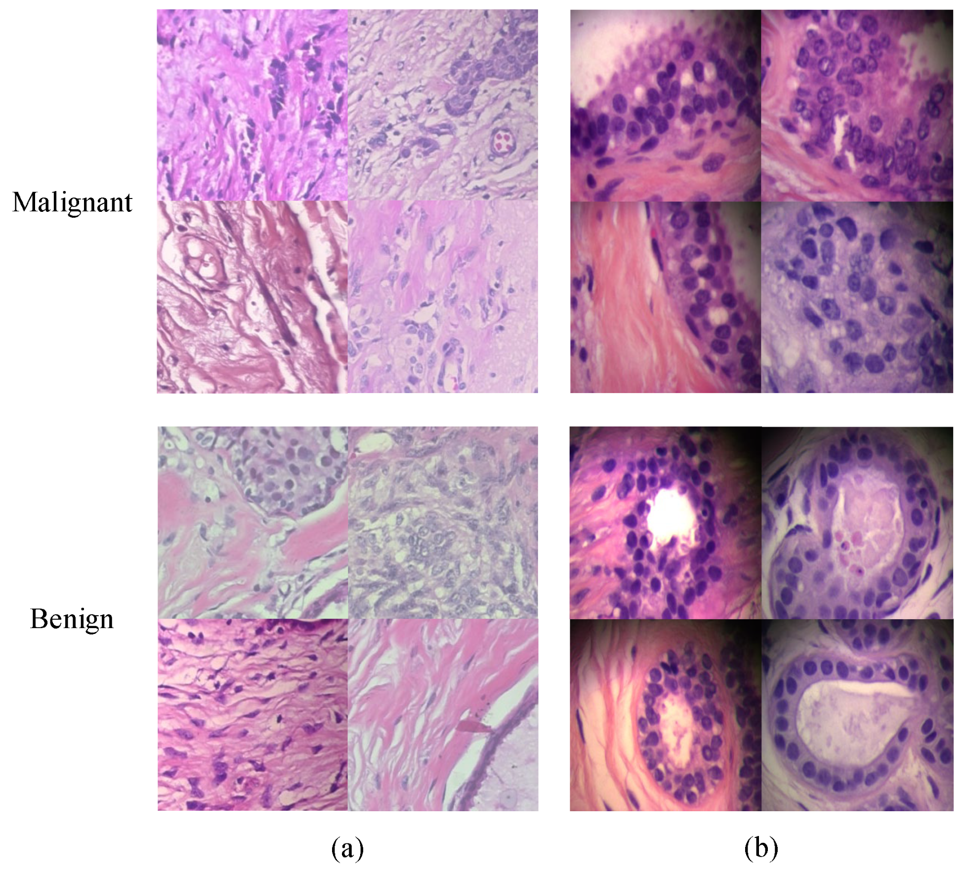
4.1. Dataset and Preprocessing

The datasets used in the AER-SSDA experiment contained a publicly available breast histopathological image dataset (BreakHis) and a private breast cancer dataset (SNL). The BreakHis dataset consisted of 7909 breast histopathological images from 82 patients [31]. The H&E-stained slides were collected at four magnification scales (40×, 100×, 200×, 400×) and the 200× images were used for this study. The private dataset was obtained from normal, uninvolved (cytopathological normal cells from malignant patients), and malignant breast tissue stained by H&E. The dataset contained 134 breast histopathological images with a resolution of 512 × 512, including 87 of normal cells, 23 of malignant cells, and 24 of cytopathological normal cells. For the experiment, the three types of histopathological samples were combined into two categories, namely 89 normal images and 47 malignant images. The representative images of the dataset samples are shown in Figure 2.
All of the BreakHis samples were cut into non-overlapping samples with a resolution of 230  ×  230 during the dataset preprocessing. SNL dataset samples were divided into overlapping samples with a resolution of 230  ×  230 at a step of 40. The number of samples before and after cutting is shown in Table 3. Before input to the network for training, all samples were normalized as well as scaled and cut into 224  ×  224 pixels. To meet the requirements of semi-supervised domain adaption training, all target domain samples were divided into training and test sets by 7 to 3. Most of the target domain samples without labels and a small portion of samples with labels were fed into the network for training with a labeled ratio of  η . For the target domain dataset, 70% of the histopathological images were randomly selected as the training set and the remaining 30% as the test set. After obtaining the classification results of the patches, the decision fusion was performed to obtain the image-level classification prediction labels.

4.2. Experiment Environment and Parameter Setting

This experiment was operated in Ubuntu 18.06, and implemented on a workstation equipped with GeForce GTX 3080ti 32GB GPU and Intel(R) Core (TM) i7-8700 @3.2 GHz CPU. The program was implemented using Python 3.6 and PyTorch 1.7.0. Following previous work [17], the batch size was 32, the training epoch was set to 30, and the learning rate was set to 0.0001. After parameter tuning by Bayesian optimization, the corresponding parameters  α β , and  γ  were set to 0.01, 0.25, and 0.001, respectively. The labeled sample ratio of the target domain  η  was set to 0.2. A 10-fold cross validation was used to verify the validity of the model.

4.3. Evaluation Metrics

The proposed AER-SSDA algorithm used binary classification tasks to distinguish benign from malignant breast histopathological images, with evaluation metrics including F1 score, accuracy, sensitivity, and specificity [17].

4.4. Result

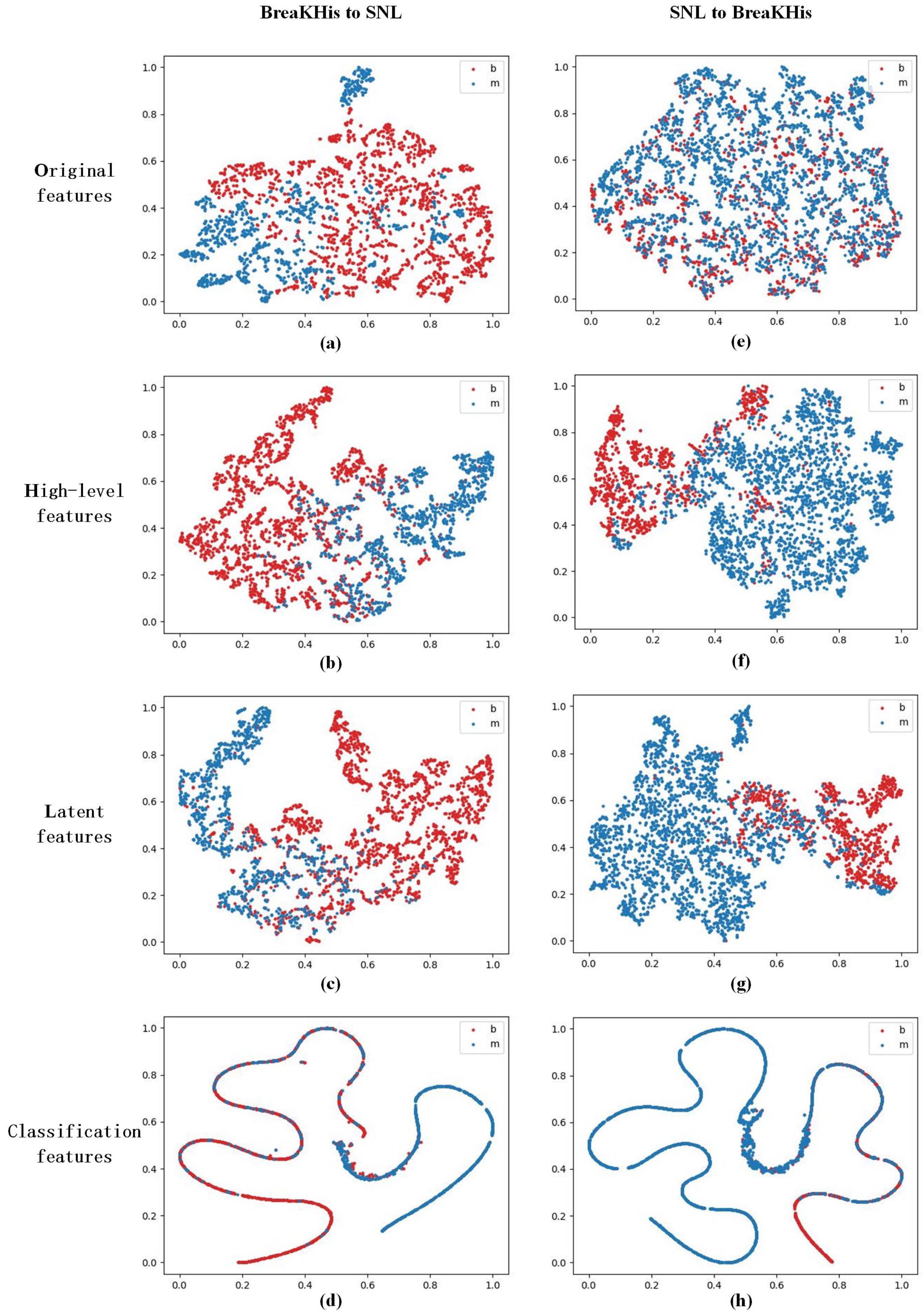
4.4.1. Feature Distribution

The features extracted from each part of the network were compared visually in order to intuitively reflect the effect of the AER-SSDA algorithm on the sample feature distribution. In this study, the network was frozen to save the parameters after the model training. The t-distributed stochastic neighbor embedding (t-SNE) [32] was used to visualize the target domain feature distribution.
Figure 3 presents the original feature distribution, high-level feature distribution, auto-encoder latent feature distribution, and classifier feature distribution of the target domain dataset. In this figure, red scatter points represent benign breast tissue pathology image samples, while blue scatter points represent malignant breast tissue pathology image samples for each feature distribution plot. The first column of the t-SNE feature distribution plots shows the feature distribution when the SNL dataset is the target domain, and the second column shows the feature distribution when the BreakHis dataset is the target domain. The first row of two feature distribution plots (a) and (e) displays the feature distribution of original images without network processing. It can be observed that there is significant overlap between benign and malignant samples, resulting in the worst separability. The second row of two feature distribution plots (b) and (f) exhibits the high-level feature distribution of histopathological images after passing through a pre-trained deep network. Samples of the same class exhibit a large radial distribution, and there is a certain separation between different classes. The separability between samples has been improved to a certain degree. The third row of two feature distribution plots (c) and (g) demonstrates the latent feature distribution after feature learning and compression through auto-encoder encoding. Compared to (b) and (f), the aggregation degree of the same class sample points becomes higher, the distance between the centers of the two classes increases, and the classification boundary becomes clearer. The images in the last row (d) and (h) show the latent feature distribution after processing by the label discriminator. Compared to the images in the first three rows, the scatter plots of the two different classes have the clearest classification boundary, and the separability between the two classes reaches the highest level. The distribution characteristics and differences in the features among the different samples indicate that the proposed AER-SSDA algorithm can effectively mine information beneficial for classification during compressed representation learning and feature reconstruction.

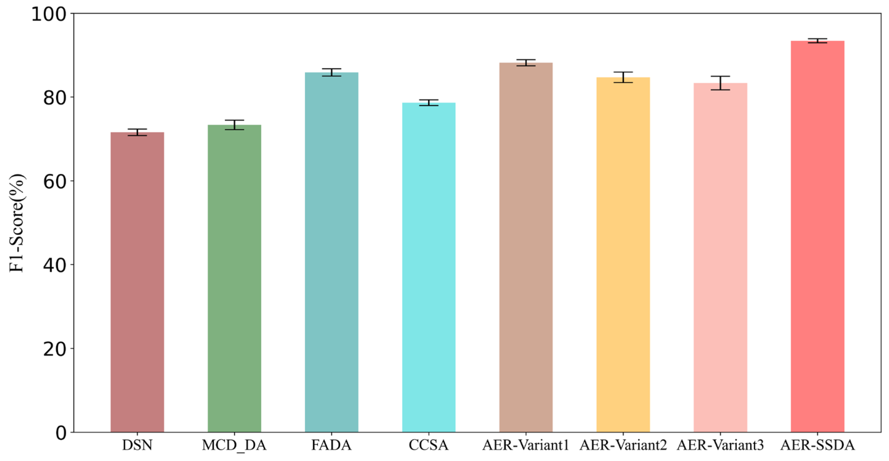
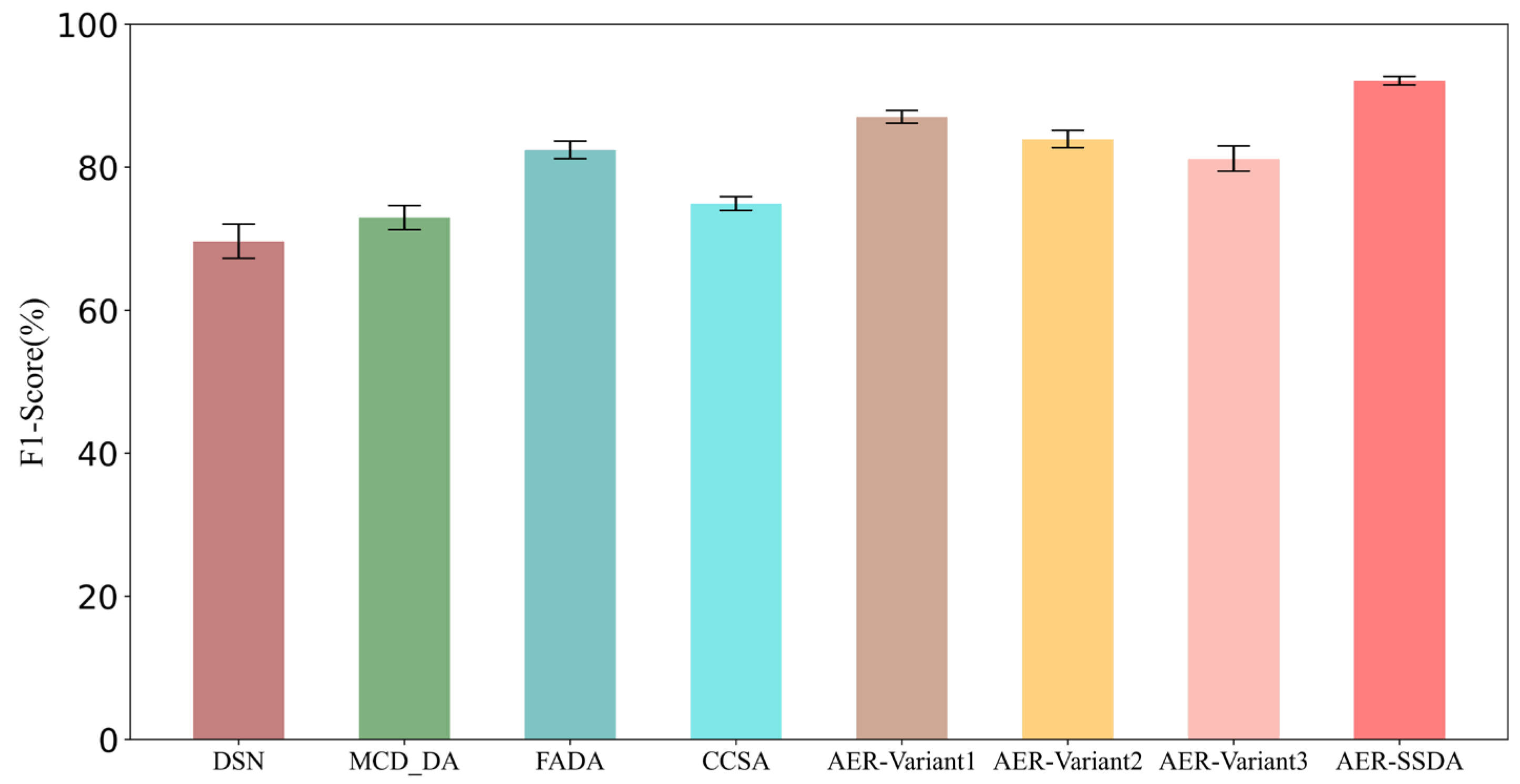
4.4.2. Comparative Experiment

To validate the effectiveness of our proposed algorithm (AER-SSDA), we compared it with several other domain adaptation algorithms. The experiments utilized the BreakHis dataset and the SNL dataset to conduct bidirectional domain adaptation classification experiments, verifying the effectiveness of the method through these bidirectional experiments.
The comparison algorithms included two unsupervised domain adaptation algorithms (DSN [33] and MCD_DA [34]), as well as two semi-supervised domain adaptation algorithms (FADA [35] and CCSA [36]). Among them, DSN and FADA are also reconstruction-based domain adaptation algorithms.
The experimental results from the BreakHis dataset to the SNL dataset are shown in Table 4. The proposed AER-SSDA algorithm exhibited the best experimental results (F1 score: 93.40%, accuracy: 95.24%, sensitivity: 94.66%, specificity: 95.56%), fully demonstrating the effectiveness of this method. Due to the lack of target sample labels that can provide classification guidance during training, the unsupervised domain adaptation methods, DSN (F1 score: 71.58%, accuracy: 64.87%, sensitivity: 61.60%, specificity: 73.22%) and MCD_DA (F1 score: 73.34%, accuracy: 75.03%, sensitivity: 90.20%, specificity: 66.14%), performed significantly worse than the proposed AER-SSDA algorithm. Compared with the other two semi-supervised domain adaptation methods, CCSA (F1 score: 78.63%, accuracy: 78.07%, sensitivity: 80.12%, specificity: 76.35%) and FADA (F1 score: 85.86%, accuracy: 80.43%, sensitivity: 82.65%, specificity: 74.78%), the proposed AER-SSDA algorithm demonstrated a stronger learning ability in semi-supervised domain adaptation tasks. This is attributed to the proposed auto-encoder, which learns more useful information for classification within a single domain during the feature extraction and reconstruction task, enhancing the representation ability of intra-domain features. When aligning multiple feature representations during the encoding–decoding process, it measures and reduces the differences in feature distributions between the source and target domains. This facilitates the transfer of labeled feature representations from the source domain to the target domain, thereby improving the classification performance of the model.
Table 5 presents the experimental results of the comparison algorithms from SNL to BreakHis. Due to the decrease in the number of source domain samples, leading to a reduction in the knowledge transferable to the target domain, the model’s classification performance declined. However, compared with other comparison methods, the proposed AER-SSDA algorithm still demonstrated better performance. This further validates the effectiveness of the model and algorithm. The experiments showed that the proposed AER-SSDA achieved the best performance in breast histopathological image classification tasks.

4.4.3. Ablation Experiment

To demonstrate the effectiveness of each key component in the algorithm, we designed three ablation variants: AER-Variant1, AER-Variant2, and AER-Variant3, for comparison with the proposed algorithm. Compared to the proposed algorithm, AER-Variant1 removes the domain similarity loss generated during the domain discrimination process; in other words, it removes loss term  L s i m i l a r i t y . AER-Variant2 explores the impact of the auto-encoder structure on experimental results by conducting domain adaptation training without reconstruction loss; in other words, it removes loss term  L r e c o n . AER-Variant3 removes both the domain discriminator, the auto-encoder and the corresponding loss function; in other words, it removes loss term  L M M D .
Table 6 presents the experimental results of the ablation variants from BreakHis to SNL. On the BreakHis -to-SNL dataset, the experimental results of the three ablation variants, AER-Variant1 (F1 score: 88.17%, accuracy: 90.96%, sensitivity: 93.33%, specificity: 89.63%), AER-Variant2 (F1 score: 84.70%, accuracy: 88.57%, sensitivity: 87.98%, specificity: 88.89%), and AER-Variant3 (F1 score: 83.32%, accuracy: 87.62%, sensitivity: 85.33%, specificity: 88.86%), demonstrated the necessity and importance of each part of the model. The results of AER-Variant1 showed that the similarity loss generated by the domain discriminator could blur the domain discriminative information in the encoder’s feature representations and enhance the model’s overall adversarial learning capability. AER-Variant2 replaced the auto-encoder embedding with a fully connected network with the same network parameters. The experimental results indicate that the proposed auto-encoder reconstruction domain adaptation model is not merely a simple compressed representation for feature extraction. In a series of feature transformations during encoding and decoding, the auto-encoder learns abstract information about histopathological images under the constraint of feature reconstruction loss, which can more effectively mine and learn the classification information of the samples. The experimental results of AER-Variant3 demonstrated that the domain similarity loss and high-level feature reconstruction loss could cooperate with each other. The analysis of the above ablation variants proves the effectiveness of the overall algorithm and its components in the domain adaptation experiment from BreakHis to SNL.
Table 7 presents the experimental results of the ablation variants from SNL to BreakHis. Due to the reduction in the number of source domain samples, the model’s classification performance declined. However, compared to other ablation variants, the proposed AER-SSDA algorithm still exhibited a better performance. This further demonstrates the effectiveness of each part of the model and algorithm. Every component in the model and loss terms is important and indispensable, and the absence of any one of them can lead to a decrease in model performance.

4.4.4. Discussion of Experimental Results

The experimental results reveal that the proposed AER-SSDA method exhibited the best classification performance. Compared to unsupervised domain adaptation methods DSN and MCD_DA, it achieved significant improvements in the results, indicating that using a small number of labeled target samples can enhance domain adaptation performance. When compared to semi-supervised domain adaptation methods FADA and CCSA, the proposed AER-SSDA method demonstrated stronger capabilities in addressing overfitting and under-training issues. This may be attributed to the fact that the domain adaptation with auto-encoder reconstruction can more effectively learn classification-beneficial information from the extracted features. Compared to AER-Variant1, AER-Variant2, and AER-Variant3, feature reconstruction enriches the useful information for classification, while the similarity loss enhances the network’s ability to extract information and minimizes cross-domain differences. The F1 score results of the comparative experiments and ablation experiments are presented in Figure 4 (BreakHis to SNL) and Figure 5 (SNL to BreakHis), which clearly demonstrate the performance advantages of the proposed AER-SSDA algorithm.
The statistical p-value tests based on accuracy for the AER-SSDA algorithm compared to the competitive and ablation algorithms are shown in Table 8 (BreakHis to SNL) and Table 9 (SNL to BreakHis). This indicates that the experimental results of the AER-SSDA algorithm are statistically significant compared to the comparative and ablation experiments, further proving that the AER-SSDA algorithm has more advantages than other algorithms in the feature reconstruction-based domain adaptation classification tasks.

5. Conclusions

In this study, an auto-encoder reconstructed semi-supervised domain adaption for a histopathological image classification algorithm (AER-SSDA) was proposed. The feature extractor, auto-encoder, domain discriminator, and sample classifier were built and performed reconstructed domain adaptation learning for the classification task of patch-level samples. First, the convolutional feature extractor pre-trained by thr ImageNet dataset performed high-level feature extraction. Subsequently, the extracted features were reconstructed by the auto-encoder. The encoder and decoder completed the information mining, representation learning, and feature reconstruction, and in the process, the original features, latent features, and reconstructed features were minimized for inter-domain distribution differences. Then, the latent features from the auto-encoder were fed to the domain discriminator and sample classifier for domain confusion and patch sample classification, respectively. Finally, the predicted labels of the whole test image were obtained by decision fusion. The experimental results of the proposed AER-SSDA method demonstrated better classification performance compared with other methods, and it has potential for clinical applications.
Despite achieving promising results on the pathological image datasets, our work still has certain limitations. We designed an auto-encoder for sample reconstruction and a feature extraction network specifically for pathological images, but we did not explore the impact of diversified network structures on image classification outcomes. In future work, we will further explore different network structures for feature extraction and sample reconstruction. Although we tested our method on two pathological image datasets and obtained good results, we have not yet explored its application on larger datasets. In the future, we plan to extend our method to large datasets and further investigate the effectiveness of the model on other types of medical images, such as CT images.

Author Contributions

Conceptualization, P.W.; methodology, J.Z. and Y.G.; supervision, P.W. and Y.L.; software, formal analysis, writing—original draft preparation, J.Z.; writing—reviewing and editing, P.L. All authors have read and agreed to the published version of the manuscript.

Funding

We are grateful for the support of the National Natural Science Foundation of China NSFC (No. U21A20448, and 72001032); Chongqing Traditional Chinese Medicine Innovation Team Construction Project (2023110002); and the research fund of Chongqing (CSTB2021TIAD-KPX0069, CSTB2023TIAD-ZXX0049).

Institutional Review Board Statement

Not applicable.

Informed Consent Statement

Informed consent was obtained from all subjects involved in the study.

Data Availability Statement

The original contributions presented in this study are included in the article. Further inquiries can be directed to the corresponding author.

Conflicts of Interest

The authors declare no conflicts of interest.

References

  1. Sudharshan, P.J.; Petitjean, C.; Spanhol, F.; Oliveira, L.E.; Heutte, L.; Honeine, P. Multiple Instance Learning for Histopathological Breast Cancer Image Classification. Expert Syst. Appl. 2019, 117, 103–111. [Google Scholar] [CrossRef]
  2. Alirezazadeh, P.; Hejrati, B.; Monsef, A.; Fathi, A. Representation Learning-based Unsupervised Domain Adaptation for Classification of Breast Cancer Histopathology Images. Biocybern. Biomed. Eng. 2018, 38, 671–683. [Google Scholar] [CrossRef]
  3. Xu, B.; Liu, J.; Hou, H.; Liu, B.; Garibaldi, B.; Ellis, I.O.; Green, A.; Shen, L.; Qiu, G. Attention by Selection: A Deep Selective Attention Approach to Breast Cancer Classification. IEEE Trans. Med. Imaging 2019, 39, 1930–1941. [Google Scholar] [CrossRef] [PubMed]
  4. Litjens, G.; Sanchez, C.I.; Timofeeva, N.; Hermsen, M.; Nagtegaal, I.; Kovacs, I.; Hulsbergen, C.; Bult, P.; Ginneken, B.; Laak, G. Deep Learning as a Tool for Increased Accuracy and Efficiency of Histopathological Diagnosis. Sci. Rep. 2016, 6, 26286. [Google Scholar] [CrossRef]
  5. Anwar, S.M.; Majid, M.; Qayyum, A.; Awais, M.; Alnowami, M.; Khan, M. Medical Image Analysis Using Convolutional Neural Networks: A Review. J. Med. Syst. 2018, 42, 226. [Google Scholar] [CrossRef] [PubMed]
  6. Alom, M.Z.; Yakopcic, C.; Nasrin, S.; Taha, T.; Asari, V. Breast Cancer Classification from Histopathological Images with Inception Recurrent Residual Convolutional Neural Network. J. Digit. Imaging 2019, 32, 605–617. [Google Scholar] [CrossRef] [PubMed]
  7. Gandomkar, Z.; Brennan, P.C.; Mello-Thoms, C. MuDeRN: Multi-category Classification of Breast Histopathological Image Using Deep Residual Networks. Artif. Intell. Med. 2018, 88, 14–24. [Google Scholar] [CrossRef] [PubMed]
  8. Gao, Z.; Lu, Z.; Wang, J.; Ying, S.; Shi, J. A Convolutional Neural Network and Graph Convolutional Network Based Framework for Classification of Breast Histopathological Images. IEEE J. Biomed. Health Inform. 2022, 26, 3163–3173. [Google Scholar] [CrossRef] [PubMed]
  9. Quinones, W.R.; Ashraf, M.; Yi, M.Y. Impact of Patch Extraction Variables on Histopathological Imagery Classification using Convolution Neural Networks. In Proceedings of the 2021 International Conference on Computational Science and Computational Intelligence (CSCI), Las Vegas, NV, USA, 15–17 December 2021; pp. 1176–1181. [Google Scholar]
  10. Li, J.; Zhang, J.; Sun, Q.; Zhang, H.; Dong, J.; Che, C.; Zhang, Q. Breast Cancer Histopathological Image Classification Based on Deep Second-order Pooling Network. In Proceedings of the 2020 International Joint Conference on Neural Networks (IJCNN) held as part of the IEEE World Congress on Computational Intelligence (IEEE WCCI), Glasgow, UK, 19–24 July 2020; pp. 1–7. [Google Scholar]
  11. Kumar, A.; Sharma, A.; Bharti, V.; Singh, A.; Singh, S.; Saxena, S. MobiHisNet: A Lightweight CNN in Mobile Edge Computing for Histopathological Image Classification. IEEE Internet Things J. 2021, 8, 17778–17789. [Google Scholar] [CrossRef]
  12. Gul, A.G.; Cetin, O.; Reich, C.; Flinner, N.; Prangemeier, T.; Koeppl, H. Histopathological Image Classification Based on Self-supervised Vision Transformer and Weak Labels. In Proceedings of the SPIE Journal of Medical Image 2022: Digital and Computational Pathology, San Diego, CA, USA, 20 February–28 March 2022; p. 12039. [Google Scholar]
  13. Huang, Y.; Zheng, H.; Liu, C.; Ding, X.; Rohde, G. Epithelium-Stroma Classification via Convolutional Neural Networks and Unsupervised Domain Adaptation in Histopathological Images. IEEE J. Biomed. Health Inform. 2017, 21, 1625–1632. [Google Scholar] [CrossRef]
  14. Yao, T.; Pan, Y.; Ngo, C.-W.; Li, H.; Mei, T. Semi-supervised Domain Adaptation with Subspace Learning for Visual Recognition. In Proceedings of the IEEE Conference on Computer Vision and Pattern Recognition (CVPR), Boston, MA, USA, 7–12 June 2015; pp. 2142–2150. [Google Scholar]
  15. Xia, T.; Kumar, A.; Feng, D.; Kim, J. Patch-level Tumor Classification in Digital Histopathology Images with Domain Adapted Deep Learning. In Proceedings of the Annual International Conference of the IEEE Engineering in Medicine and Biology Society, Honolulu, HI, USA, 18–21 July 2018; IEEE Engineering in Medicine and Biology Society. Annual International Conference. pp. 644–647. [Google Scholar]
  16. Zhang, Y.; Zhang, H.; Deng, B. Semi-supervised Models are Strong Unsupervised Domain Adaptation Learners. arXiv 2021, arXiv:2106.00417. [Google Scholar]
  17. Wang, P.; Li, P.; Li, Y.; Xu, J.; Jiang, M. Classification of Histopathological Whole Slide Images Based on Multiple Weighted Semi-supervised Domain Adaptation. Biomed. Signal Process. Control 2022, 73, 103400. [Google Scholar] [CrossRef]
  18. Medela, A.; Picon, A.; Saratxaga, C.L.; Belar, O.; Cabezon, V.; Cicchi, R.; Bilbao, R.; Glover, B. Few Shot Learning in Histopathological Images: Reducing the Need of Labeled Data on Biological Datasets. In Proceedings of the 16th IEEE International Symposium on Biomedical Imaging (ISBI), Venice, Italy, 8–11 April 2019; pp. 1860–1864. [Google Scholar]
  19. Li, L.; Zhang, Z. Semi-Supervised Domain Adaptation by Covariance Matching. IEEE Trans. Pattern Anal. Mach. Intell. 2019, 41, 2724–2739. [Google Scholar] [CrossRef]
  20. Ahn, E.; Kumar, A.; Fulham, M.; Feng, D.; Kim, J. Unsupervised Domain Adaptation to Classify Medical Images Using Zero-Bias Convolutional Auto-Encoders and Context-Based Feature Augmentation. IEEE Trans. Med. Imaging 2020, 39, 2385–2394. [Google Scholar] [CrossRef] [PubMed]
  21. Bian, X.; Luo, X.; Wang, C.; Liu, W.; Lin, X. DDA-Net: Unsupervised Cross-modality Medical Image Segmentation via Dual Domain Adaptation. Comput. Methods Programs Biomed. 2021, 213, 106531. [Google Scholar] [CrossRef] [PubMed]
  22. Ahn, E.; Kumar, A.; Feng, D.; Fulham, M.; Kim, J. Unsupervised Deep Transfer Feature Learning for Medical Image Classification. In Proceedings of the 2019 IEEE 16th International Symposium on Biomedical Imaging (ISBI 2019), Venice, Italy, 8–11 April 2019; pp. 1915–1918. [Google Scholar]
  23. Zhao, H.; Ren, T.; Wang, C.; Yang, X.; Wen, Y. Multi-context Unsupervised Domain Adaption for HEp-2 Cell Classification Using Maximum Partial Classifier Discrepancy. J. Supercomput. 2022, 78, 14362–14380. [Google Scholar] [CrossRef]
  24. Yi, Z.; Zhang, H.; Tan, P.; Gong, M. DualGAN: Unsupervised Dual Learning for Image-to-Image Translation. In Proceedings of the 2017 IEEE International Conference on Computer Vision (ICCV), Venice, Italy, 22–29 October 2017; pp. 2868–2876. [Google Scholar]
  25. Zhu, J.-Y.; Park, T.; Isola, P.; Efros, A. Unpaired Image-to-Image Translation Using Cycle-Consistent Adversarial Networks. In Proceedings of the IEEE International Conference on Computer Vision (ICCV), Venice, Italy, 22–29 October 2017; pp. 2242–2251. [Google Scholar]
  26. Jue, J.; Hu, J.; Neelam, T.; Andreas, R.; Sean, B.; Joseph, D.; Harini, V. Integrating Cross-modality Hallucinated MRI with CT to Aid Mediastinal Lung Tumor Segmentation. Med. Image Comput. Comput. Assist. Interv. 2019, 11769, 221–229. [Google Scholar]
  27. Roels, J.; Hennies, J.; Saeys, Y.; Philips, W.; Kreshuk, A. Domain Adaptive Segmentation in Volume Electron Microscopy Imaging. In Proceedings of the 16th IEEE International Symposium on Biomedical Imaging (ISBI), Venice, Italy, 8–11 April 2019; pp. 1519–1522. [Google Scholar]
  28. Voigt, B.; Fischer, O.; Schilling, B.; Krumnow, C.; Herta, C. Investigation of semi-and self-supervised learning methods in the histopathological domain. J. Pathol. Inform. 2023, 14, 100305. [Google Scholar] [CrossRef] [PubMed]
  29. Zhu, Y.; Hu, X.; Zhang, Y.; Li, P. Semi-Supervised Representation Learning: Transfer Learning with Manifold Regularized Auto-Encoders. In Proceedings of the 9th IEEE International Conference on Big Knowledge (ICBK), Singapore, 17–18 November 2018; pp. 83–90. [Google Scholar]
  30. He, Y.; Carass, A.; Zuo, L.; Dewey, B.; Prince, J. Autoencoder Based Self-Supervised Test-time Adaptation for Medical Image Analysis. Med. Image Anal. 2021, 72, 102136. [Google Scholar] [CrossRef] [PubMed]
  31. Spanhol, A.F.; Oliveira, S.L.; Petitjean, C.; Heutte, L. A Dataset for Breast Cancer Histopathological Image Classification. IEEE Trans. Biomed. Eng. 2016, 63, 1455–1462. [Google Scholar] [CrossRef] [PubMed]
  32. Van Der Maaten, L.; Hinton, G. Visualizing Data Using t-SNE. J. Mach. Learn. Res. 2008, 9, 2579–2605. [Google Scholar]
  33. Bousmalis, K.; Silberman, N.; Krishnan, D.; Erhan, D. Domain Separation Networks. In Proceedings of the 30th International Conference on Neural Information Processing Systems, Barcelona, Spain, 5–10 December 2016; pp. 343–351. [Google Scholar]
  34. Wang, W.; Wang, H.; Zhang, Z.; Zhang, C.; Gao, Y. Semi-Supervised Domain Adaptation via Fredholm Integral Based Kernel Methods. Pattern Recognit. 2019, 85, 185–197. [Google Scholar] [CrossRef]
  35. Motiian, S.; Jones, Q.; Iranmanesh, S.M.; Doretto, G. Few-Shot Adversarial Domain Adaptation. In Proceedings of the 31st Annual Conference on Neural Information Processing Systems (NIPS), Long Beach, CA, USA, 4–9 December 2017; pp. 6673–6683. [Google Scholar]
  36. Motiian, S.; Piccirilli, M.; Adjeroh, D.A.; Doretto, G. Unified Deep Supervised Domain Adaptation and Generalization. In Proceedings of the 16th IEEE international Conference on Computer Vision (ICCV), Venice, Italy, 22–29 October 2017; pp. 5716–5726. [Google Scholar]
Figure 1. The diagram of auto-encoder reconstructed semi-supervised domain adaptation for breast histopathological image classification.
Applsci 14 11802 g001
Figure 2. Representative breast histopathological image of two datasets: (a) BreakHis, (b) private dataset.
Applsci 14 11802 g002
Figure 3. Feature visualization of different feature distribution of the target domain images (BreakHis to SNL: (ad); SNL to BreakHis to SNL: (eh)).
Applsci 14 11802 g003
Figure 4. Comparison of classification results with different methods (BreakHis to SNL).
Applsci 14 11802 g004
Figure 5. Comparison of classification results with different methods (SNL to BreakHis).
Applsci 14 11802 g005
Table 1. Summary of related research work.
AuthorDatasetEvaluation IndicatorsModelDomain Adaptation Method
Alom et al. [6]BreakHisAccuracyIRRCNNNone
Gandomkar et al. [7]Mitosis-Atypia databaseAccuracyBased on ResNetNone
Li et al. [10]BreakHisIRR, PRRDSoPNNone
Kumar et al. [11]BreakHisAccuracyMobiHisNetNone
Wang et al. [17]DigestPath 2019Accuracy,
sensitivity,
specificity,
HisNetSemi-supervised domain adaptation based on manifold regularization
Medela et al. [18]UMCMAccuracy,
sensitivity,
specificity
Siamese Neural NetworkSemi-supervised domain adaptation based on class distance metric
Table 2. Symbol description.
SymbolMeaning
  ( X S , Y S ) Annotated source domain dataset
  ( X T l , Y T l ) Annotated target domain dataset
  ( X T u , Y T u ) Unannotated target domain dataset
  X i n Intermediate layer output of neural networks
  f Activation function of neural networks
  L m Total loss of the algorithm
  L t a s k Loss for classification task
  L r e c o n Loss for reconstruction task
  L s i m i l a r i t y Domain similarity loss
  L M M D Domain adaptive feature alignment loss
  α , β , γ Hyperparameters of the network
Table 3. The number of images of datasets.
DatasetClassTotal NumberPatchesTrainTest
BreakHisMalignant1390834058382502
Benign623373826161122
SNLMalignant4730082048960
Benign87556838401728
Table 4. The experimental results of different comparative algorithms (BreakHis to SNL)
MethodF1 Score (%)Accuracy (%)Sensitivity (%)Specificity (%)
DSN [33]71.58 ± 0.7864.87 ± 1.2461.60 ± 2.3173.22 ± 1.72
MCD_DA [34]73.34 ± 1.1175.03 ± 1.4990.20 ± 1.7666.14 ± 2.94
FADA [35]85.86 ± 0.8880.43 ± 0.6082.65 ± 0.9274.78 ± 0.89
CCSA [36]78.63 ± 0.6978.07 ± 0.7380.12 ± 1.0876.35 ± 1.43
AER-SSDA93.40 ± 0.4895.24 ± 0.3294.66 ± 0.8795.56 ± 1.27
The bold numbers in the table represent the best comparison results.
Table 5. The experimental results of different comparative algorithms (SNL to BreakHis)
MethodF1 Score (%)Accuracy (%)Sensitivity (%)Specificity (%)
DSN [33]69.64 ± 2.3977.78 ± 2.3571.11 ± 3.1781.48 ± 2.83
MCD_DA [34]72.95 ± 1.6874.74 ± 1.4695.17 ± 1.2763.38 ± 4.58
FADA [35]82.42 ± 1.2378.25 ± 1.0779.88 ± 1.6473.46 ± 2.04
CCSA [36]74.91 ± 0.9874.65 ± 0.8574.58 ± 1.6775.45 ± 1.52
AER-SSDA92.08 ± 0.5989.47 ± 0.4788.87 ± 1.1989.14 ± 1.22
The bold numbers in the table represent the best comparison results.
Table 6. The experimental results of different ablation algorithms (BreakHis to SNL).
MethodLossF1 Score (%)Accuracy (%)Sensitivity (%)Specificity (%)
  L s i m i l a r i t y   L r e c o n   L M M D
AER-Variant1 88.17 ± 0.7190.96 ± 0.6793.33 ± 1.2189.63 ± 1.37
AER-Variant2 84.70 ± 1.2588.57 ± 1.0187.98 ± 2.1288.89 ± 1.46
AER-Variant3 83.32 ± 1.6387.62 ± 2.0985.33 ± 2.7588.86 ± 1.94
AER-SSDA93.40 ± 0.4895.24 ± 0.3294.66 ± 0.8795.56 ± 1.27
In the table, a ✓ below the loss item indicates that this loss exists, and the absence of a ✓ represents that this loss item is discarded in the total loss function. The bold numbers in the table represent the best comparison results.
Table 7. The experimental results of different ablation algorithms (SNL to BreakHis).
MethodLossF1 Score (%)Accuracy (%)Sensitivity (%)Specificity (%)
  L s i m i l a r i t y   L r e c o n   L M M D
AER-Variant1 87.02 ± 0.8684.17 ± 0.9582.40 ± 1.4388.13 ± 1.37
AER-Variant2 83.89 ± 1.2181.23 ± 1.4175.53 ± 2.3887.80 ± 1.89
AER-Variant3 81.17 ± 1.7677.26 ± 1.8368.71 ± 3.4188.75 ± 1.53
AER-SSDA92.08 ± 0.5989.47 ± 0.4788.87 ± 1.1989.14 ± 1.22
In the table, a ✓ below the loss item indicates that this loss exists, and the absence of a ✓ represents that this loss item is discarded in the total loss function. The bold numbers in the table represent the best comparison results.
Table 8. The statistical result of the p-value (BreakHis to SNL).
Methodsp-Value (%)
DSN [33]   1.77 × 10 - 11
MCD_DA [34]   1.81 × 10 - 9
FADA [35]   3.5 × 10 - 11
CCSA [36]   3.82 × 10 - 11
AER-Variant 1   1.24 × 10 - 6
AER-Variant 2   6.3 × 10 - 7
AER-Variant 3   4.14 × 10 - 5
Table 9. The statistical result of the p-value (SNL to BreakHis).
Methodsp-Value (%)
DSN [33]   4.42 × 10 - 6
MCD_DA [34]   2.33 × 10 - 8
FADA [35]   2.33 × 10 - 8
CCSA [36]   5.95 × 10 - 10
AER-Variant 1   3.67 × 10 - 6
AER-Variant 2   1.67 × 10 - 6
AER-Variant 3   5.14 × 10 - 7
Disclaimer/Publisher’s Note: The statements, opinions and data contained in all publications are solely those of the individual author(s) and contributor(s) and not of MDPI and/or the editor(s). MDPI and/or the editor(s) disclaim responsibility for any injury to people or property resulting from any ideas, methods, instructions or products referred to in the content.

