Abstract
The artificial freezing construction technology, compared to other methods, offers several advantages, including superior waterproofing capabilities and the absence of environmental pollution. This technique is particularly prevalent in the construction of tunnels in challenging environments, where the dynamics of the freezing temperature field during the freezing process have consistently been a key area of interest during actual construction activities. In the Sanya Estuary Channel Submarine Tunnel Project, a three-dimensional transient model was developed using COMSOL finite element software to deeply analyze the formation and temperature distribution of the permafrost curtain. Two alternative schemes were designed to improve the original design by optimizing the layout of the permafrost pipeline. Comparative analysis shows that the isotherm −10 °C intersected at 14 days in the original scheme, 23 days in Optimized Scheme 1, and 24 days in Optimized Scheme 2, indicating a 10-day delay in Scheme 2 versus the original, yet still meeting the 25-day deadline. After 40 days of active freezing, the greatest difference in permafrost curtain thickness was observed at the east wall (downstream), with Scheme 2 differing by 1.05 m from the original and by 0.23 m from Scheme 1. Scheme 2 achieved an average permafrost curtain thickness of 4.18 m around the tunnel, exceeding the 3.5-m design requirement. The mean temperatures in the strong and weak freezing zones of Scheme 2 were below −10 °C and −8 °C, respectively, aligning with design standards. Given the conservative nature of the initial plan, Optimized Scheme 2 is highly practical for implementation and offers significant cost savings.
1. Introduction
The rapid urban economic development is characterized by a significant influx of people to economically thriving cities, leading to increased population pressure and insufficient above-ground space. Consequently, many countries are turning to the full development and utilization of underground space as a preferred solution to this issue [1,2]. However, the development of underground space faces numerous complex engineering challenges. Particularly in eastern China, where the hydrological system is complex, underground engineering must also account for the effects of groundwater on construction. Conventional construction techniques are not suitable for areas rich in water and with weak strata. To address this, people have developed and proposed a method known as artificial freezing technology, which involves freezing the natural environment. This technique also referred to as the artificial freezing method, has been widely applied in water-rich and weak strata regions [3,4,5,6]. However, when the volume of construction permafrost is too large, the soil expands excessively upon freezing and produces settlement displacements when it melts [7,8,9,10]. In order to reduce the impact of frost heave and thaw settlement on construction, scholars have combined the pipe curtain method with freezing methods to create the pipe curtain freezing method [11]. The pipe curtain freezing method represents a significant advancement in artificial ground freezing technology, integrating the principles of pipe curtain technology with artificial ground freezing. In this method, the pipe curtain support structure serves as the primary load-bearing system, while the frozen soil curtain, generated through the application of artificial ground freezing technology, primarily functions as a water barrier [12,13,14,15]. The Gongbei Tunnel, a component of the Hong Kong–Zhuhai–Macao Bridge Zhuhai Link Road project, is situated in a section characterized by saturated soil, high compressibility, and high permeability. To ensure the safety of construction personnel while preserving the integrity of existing ground structures and underground utilities, the construction team adopted the pipe curtain freezing method, a technique that has been successfully applied for the first time in domestic tunnel engineering [16,17,18,19,20]. In recent years, many scholars have made some achievements in the research of the pipe curtain freezing method. Long Wei et al. conducted a numerical analysis of the freezing project for the new west ventilation shaft at Yandian No.2 Mine in Huaibei Coalfield, employing a water–heat coupling model for the freezing temperature field based on the theory of mixed media. The analysis compared field measurement data with numerical calculation results, revealing that a greater proportion of water in the soil body inside the freezing pipe circle froze into ice compared to that outside the circle. This indicates a more pronounced phase change in the soil body within the freezing pipe circle [21]. Pang Changqiang et al. conducted a study to investigate the evolution of the three-dimensional non-uniform freezing temperature field. To achieve this, they established a tunnel level freezing model test system based on the similarity criterion of hydrothermal coupling. The system was equipped with thermocouple temperature sensors to measure temperatures in three sections. The findings indicate that there are three cycles of temperature decrease curves at the measurement points: a sharp decrease, a slow decrease, and stabilization. The temperature profiles on both the primary and secondary planes of the frozen wall exhibited a V” shape [22]. Li Mengkai et al. investigated the distribution law of freezing and expansion within the seepage layer during tunnel construction using the horizontal freezing method. Their findings indicated that the rate of expansion for the upstream frozen wall was notably slower than that of the downstream wall, and the freezing temperature field was symmetrical along the seepage direction. The vertical freezing expansion displacement on the surface was observed to decrease as the tunnel depth increased, with the location of the maximum value remaining consistent with the increase in tunnel depth. [23]. Yao Zhishu and colleagues focused on the challenge of analyzing the temperature field during well drilling using the artificial freezing method in the Cretaceous formation. They conducted numerical simulations and experimental measurements of the temperature field, establishing a numerical model for the freezing project’s temperature field. This model predicted and analyzed the effective thickness of the freezing wall, the average temperature, and the wellbore wall temperature at various depths. A comparison of the measured temperatures from a test hole with those of the well wall indicated that the numerical simulation results closely matched the experimental data. [24]. Li Zhiming et al. have highlighted the issue of insufficient temperature monitoring data and the complexity of numerical models, which impede the accurate prediction of complete frozen curtains in engineering applications. They proposed a coupled thermal and humidity model to predict the dynamic formation of frozen curtains. The findings indicate that hydraulic parameters can be derived from NMR measurements. The numerical model was also validated through indoor tests under various seepage conditions [25]. Gao Guoyao and colleagues investigated the phenomenon of artificial freezing in clay–sand strata under conditions of seepage, which involves coupled processes of water–ice–salt crystallization and heat–force transfer. Their findings indicated that the profiles of ice content, crystallized salt content, and adsorbed salt content within the clay–sand formation exhibited a non-linear distribution with a pronounced curve at the interface. The higher crystallized salt content in the clay layer compared to the sand layer was attributed to the effects of water seepage and heat conduction. The distribution profile of soil deformation in the clay–sand layer was observed to be bilinear [26].
As evidenced by the existing literature, experts and scholars have conducted research on the reinforcement mechanism of the pipe curtain freezing method and the changing laws of the freezing and thawing temperature field through actual measurements, indoor experiments, and numerical simulations. Despite this, relatively few domestic projects have adopted the pipe curtain freezing method in underwater tunnel excavation, making it necessary to explore its application in this context. This paper presents a case study of the pipe curtain freezing method used in the Sanya Estuary Undersea Tunnel project, employing COMSOL finite element software (version 6.0) to establish a three-dimensional water–heat coupling model for the numerical simulation of the temperature field. The research focuses on the development and distribution laws of the permafrost curtain and temperature field of this project. The dynamic simulation of the permafrost curtain evolution is primarily concerned with its development, circular intersections, average temperature, and effective thickness changes. Based on the simulation results of the original scheme, the paper conducts an optimization design of the freezing scheme and compares the changes in the permafrost curtain thickness under the optimized scheme. The findings of this project can serve as a theoretical reference for the design of similar projects in the future.
2. Freeze Program Design
2.1. Project Overview
This design scheme for freezing is exemplified by the Sanya Estuary Channel Pipe Curtain Freezing Tunnel project. The project is situated in Tianya District, Sanya City, spanning the estuary of the Sanya River and connecting the north bank of the Hexi District with the south bank of the Luhuitou Peninsula. The construction tunnel has a total length of 3118 m. As an essential link connecting the Luhuitou Peninsula, the project is crucial for supporting the development of the southern sea area of the headquarters economy, enhancing the urban road network, improving regional transportation, and supporting the development of the South Border Sea Area of the Headquarters Economy, improving the urban road network, enhancing regional traffic, eliminating traffic bottlenecks, and easing the pressure of transit traffic in the old city. The project is surrounded by a sensitive environment, a unique geographic location, and a complex geological environment, passing through various unfavorable soil layers such as silty clay and highly permeable fine sand. The geology on the south bank is primarily composed of miscellaneous fill, clay, coral rubble (a strongly permeable layer), strongly weathered quartz sandstone, and moderately weathered quartz sandstone. On the north bank, the geology is dominated by miscellaneous fill, chalky clay, fine sand (a strongly permeable layer), and clay. Based on the conditions on both sides of the river, the tunnel in the estuary section is a single-cavity double-deck tunnel with upper and lower decks, and it is constructed using the pipe curtain freezing method.
2.2. Arrangement of Freezing Pipes and Pipe Curtain Steel Pipes
The freezing method employs a combination of freezing pipes and steel pipes, where the latter serves as a support structure. This system, which includes freezing pipes to create a permafrost curtain, effectively prevents water ingress and provides support. Based on the pipe curtain structure, the freezing curtain can be categorized into four distinct areas: the bottom plate, the west side wall, the east side wall, and the top plate. These areas are further divided into strong and weak freezing zones, each containing both types of zones (Figure 1). The strong freezing zone encompasses the inner and outer areas around the steel pipes’ cutting and connecting weld plates, with the freezing wall in this zone meeting the necessary load-bearing and water-sealing requirements at the roof pipe’s cutting. Conversely, the weak freezing zone is located around the occlusal pipes, with the freezing wall designed to resist the adverse effects of intense heat sources during roof pipe cutting and welding, ensuring closure and water-stopping requirements are met. The pipe curtain’s frozen section is equipped with steel pipes and freezing pipes in a ring direction along the tunnel, with a total of 28 steel pipes installed to minimize gaps. This setup includes eight sets of occlusal steel pipes and four independent steel pipes. The occlusal steel pipes, formed by cutting and connecting steel plates between three pipes, serve as support reinforcement through freezing. The design includes an effective permafrost curtain thickness of ≥3.5 m for both the strong and weak freezing zones, with an average temperature of ≤−10 °C in the strong zone and ≤−8 °C in the weak zone. A total of 170 freezing pipes are arranged, with 93 in the outer circle and 77 in the inner circle, maintaining a spacing of 800 mm in the strong freezing zone and 950 mm in the weak freezing zone.
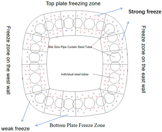
Figure 1.
The arrangement of the steel pipe and the frozen pipe in the original scheme.
3. Three-Dimensional Numerical Modelling
3.1. Basic Assumptions
For the convenience of the numerical model and the relative accuracy of the model in calculations, the following basic assumptions are made for the calculations.
- The influence of the stress field on the temperature field is neglected. Only the coupling of the seepage field and the temperature field is considered.
- The soil is a saturated, homogeneous, isotropic porous medium with a constant total porosity.
- Darcy’s law applies to the groundwater flow in the porous medium.
- The heat transfer in the frozen porous medium satisfies Fourier’s law.
- It is assumed that the initial temperature of the stratum is 18 °C, the soil is a porous saturated medium, and the soil is homogeneously distributed and homogeneous.
3.2. Model Calculation Theory
3.2.1. Temperature Field Theory
According to the basic theory of heat transfer, in the freezing process, the soil and low-temperature refrigerant exchange heat and the formation of permafrost. Seepage within the soil is frozen into ice, creating a heat transfer problem with a phase change, and the heat transfer of the porous medium is related to conduction, convection, and other factors. Under the seepage conditions of the transient temperature field, the heat conduction equation is:
where: subscripts s and f are solid and fluid, respectively; ∇ is the Hamiltonian operator; T is the temperature; C is the specific heat capacity; is the density in kg-m−3; is the convective velocity; keff is the thermal conductivity; is the solid volume fraction; Q is the other heat source sink term.
3.2.2. Percolation Field Theory
The seepage field flow direction flow rate is determined by the boundary head difference; because the soil body is a porous medium, its geometry is complex, seepage through the pore channel is discontinuous and has a slow flow rate. Therefore, seepage flow in the porous medium is usually laminar or nearly laminar flow, applicable to Darcy’s law. The formula is:
where: the subscript t denotes time; ∇ is the Hamiltonian operator; ∇P is the pressure gradient; Qm is the water source term; K is the infiltration rate of soil; is the water viscosity; is the water density; is the Darcy seepage rate.
3.2.3. Theory of Coupled Temperature and Seepage Fields
In the model boundary, the head difference is set to produce unidirectional seepage. When the seepage flow occurs in the porous media, it will produce a heat exchange phenomenon. Heat will diffuse with the seepage flow, resulting in uneven distribution of the temperature field. When the temperature field changes, the permeability coefficient of the porous media and other physical parameters will change with the temperature, and temperature constitutes a functional relationship so that the temperature field has an inverse effect on the seepage field to achieve the bi-directional coupling, the temperature field coupled with the seepage field to achieve. The coupling of the temperature field and seepage field is the process of dynamic adjustment of heat and fluid in porous media. In this study, the Heaviside function is used to describe the coupling relationship between the permeability coefficient and the temperature in the process of ice–water phase transition, and the unit leap order function is established as:
where: subscripts u and f are unfrozen and frozen soil, respectively; K is the permeability coefficient; T is the soil temperature, Td is the critical temperature of ice–water phase transition; dT is the ice–water phase transition gap.
3.3. Geometric Modelling and Meshing
This paper utilizes COMSOL to develop a transient, three-dimensional model incorporating phase change effects. The model’s geometric dimensions are determined based on the freezing range, with the dimensions set as follows: the geometric model has a length (X) of 30 m, a width (Y) of 30 m, and a height (Z) of 20 m. The model is composed of three structural parts: the soil body, the pipe curtain, and the freezing pipe. The pipe curtain consists of three pipes: the central pipe has an outer diameter of 2.1 m, while the two side pipes have an outer diameter of 2.0 m and a wall thickness of 25 mm. The independent steel pipe has an outer diameter of 2.2 m and a wall thickness of 25 mm. The three-dimensional overall model is depicted in Figure 2. The meshing adopts user-defined free tetrahedral mesh with the adaptive method in order to reduce the calculation error and improve the convergence; firstly, mesh the freezing tube to reduce its grid size in the boundary area due to not being directly affected by the freezing tube temperature change can appropriately increase the grid size, reasonable division of the grid density, this numerical model is finally the complete mesh is divided into a total of 1,215,489 number cells. The schematic of the model’s mesh division is shown in Figure 3.
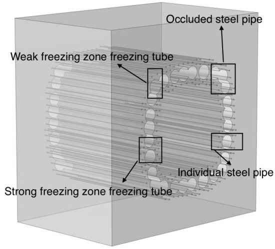
Figure 2.
Schematic diagram of the overall model.
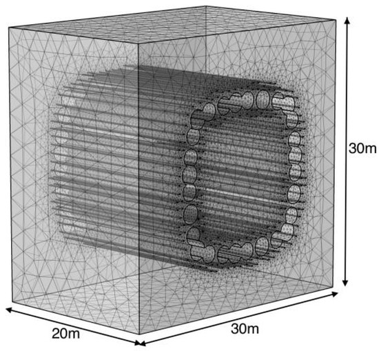
Figure 3.
Schematic diagram of meshing.
3.4. Establishment of Initial and Boundary Conditions
3.4.1. Initial Conditions
The model’s initial conditions encompass the specification of the initial temperature of the sandy soil and the determination of the seepage velocity. The initial temperature of the soil layer is set at 18 °C. The initial conditions for the seepage velocity are ascertained by the upstream and downstream head differences. Thus, the relationship between seepage velocity and head differences can be expressed by the following equation:
Formulas: V: seepage rate; K: permeability coefficient; ΔH: head difference; ΔL: hydraulic path.
3.4.2. Boundary Condition
Boundary conditions for the temperature field: all faces of the model are set as adiabatic boundaries. For the seepage field, the left (X = 0 m) and right (X = 30 m) positions of the three-dimensional model are defined as thermostatic permeable boundaries. In contrast, the remaining boundary surfaces are adiabatic impermeable boundaries. The head height can be defined based on the head difference. Groundwater flows out from the YZ plane at X = 0 and the YZ plane at X = 30. The head difference is set to 1 m, and using the mathematical formulas previously mentioned, the permeation velocity of 0.3 m/d can be calculated, thus satisfying the water flow infiltration rate requirements of the numerical model. Based on the above mathematical formulae, it is possible to calculate the infiltration rate of 0.3 m/day, respectively, ensuring the water flow infiltration rate requirements of the numerical model. The schematic diagram of the model boundary setting under the seepage condition is illustrated in Figure 4. The direction of seepage is depicted in Figure 5, with the red arrow indicating the direction of seepage.
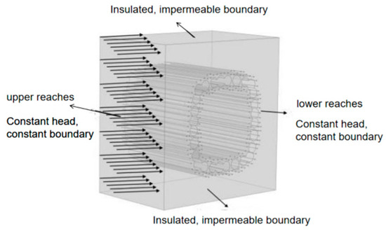
Figure 4.
Schematic diagram of boundary conditions.
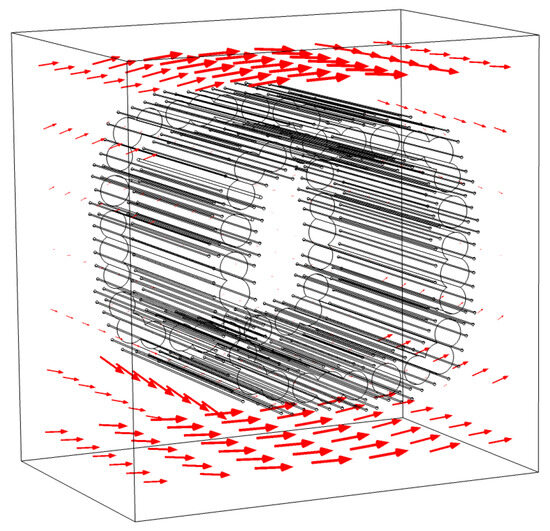
Figure 5.
Schematic diagram of seepage direction.
3.5. Selection of Relevant Parameters and Brine Cooling Programme
3.5.1. Selection of Material Parameters
Given that the project traverses through layers of powdery clay and silty soil, it was deemed necessary to model the most adverse soil conditions, drawing inspiration from experimental studies on permafrost [27]. Consequently, Table 1 presents the pertinent parameters of the soil and fluid that are integral to the simulation of the temperature field and seepage field.

Table 1.
List of relevant material parameters.
3.5.2. Salt Water Cooling Program
The cooling strategy for the brine in this project is executed according to a predefined schedule, prohibiting direct reduction of the brine temperature for recycling purposes. The model is analyzed using transient analysis, with the brine cooling plan implemented in COMSOL software through interpolating functions. The wall of the freezing tube serves as the thermal boundary condition, with the low-temperature brine inside the freezing tube acting as the temperature boundary condition. The technical parameters for the freezing tube are as follows: ① The active freezing time cycle of the freezing tube is 40 days, with each analysis step lasting 24 h (1 day); ② The initial temperature is 18 °C, which is reduced to −15 °C by the 5th day of the freezing process, and the temperature of the brine remains at −28 °C from the 10th to the 40th day, ensuring that the brine temperature is sufficiently lowered to −28 °C for smooth excavation of the submarine tunnel; ③ In the design, the average temperature of the permafrost curtain in the strong freezing zone is set at ≤ −10 °C, and the average temperature of the permafrost curtain in the weak freezing zone is ≤ −8 °C. If the temperature of the brine and the thickness of the permafrost curtain do not meet the pre-set design criteria, the duration of active freezing should be appropriately extended, with the brine cooling schedule shown in Table 2.
Table 2.
Saltwater cooling program.
Before excavation, probe holes must be opened in the frozen area to verify the temperature of the frozen soil and the thickness of the frozen wall, ensuring the normal operation of the freezing system. Based on the measured temperature data of the brine and the temperature of the measurement holes, it is determined whether there is any intersection of rings in the frozen curtain, ensuring that there is minimal pressure on the soil layer in the frozen curtain before formal excavation. Four different paths are established in the model solely to clearly indicate the cooling law of the temperature field and provide a reference for the next construction phase. For the accuracy of the numerical analysis of the temperature field of the freezing method, this group has compared the numerical analysis with many on-site measurements, with the relevant data obtained matching the expected values, proving the reliability of the current numerical simulation method. This reliability can be further supported by related literature [28,29].
4. Analysis of the Results of the Numerical Simulation of the Original Scheme
4.1. Development of Temperature Field Cloud Maps Under Seepage Conditions
To gain a better understanding of the distribution and variation of the temperature field in the freezing process, we analyzed the temperature field cloud at a cross-section of Z = 10 m. The development and distribution of the temperature field cloud at (1 d, 5 d, 15 d, 30 d, 40 d) for the Z = 10 m cross-section are illustrated in Figure 6. Examining the results from Figure 6 reveals that the development of flow lines between the frozen curtain and the groundwater clearly demonstrates the coupling between the temperature field and the seepage field. At the initial stage of freezing (1st day), freezing tubes have just initiated in the entire soil body, and the minimal cold generated by the freezing tubes is confined to the immediate vicinity of the tubes. The blue area is limited to the vicinity of the freezing tubes, with cold from the tubes not yet diffusing into the surrounding soil. At this time, groundwater flow moves from high to low heads through the entire freezing area. By the 5th day of freezing, the density of freezing tubes makes it evident that the blue color in the strong freezing area is more pronounced than in the weak freezing area in the temperature field map. The deeper blue in the temperature field cloud diagram indicates a lower average temperature in the strong freezing zone compared to the weak freezing zone, showcasing a superior freezing effect. The freezing curtain is gradually forming, and the curtain in the strong freezing zone begins to impede water flow. Groundwater flow lines start to bypass the freezing curtain, though some water flow persists within the curtain. By the 15th day of freezing, it is evident that most of the frozen area has reached the freezing temperature, and the frozen soil curtain is largely formed, obstructing groundwater flow. At this point, there is no groundwater flow within the frozen soil curtain, indicating that the curtain can effectively hinder groundwater flow. On the 30th day of freezing, the permafrost curtain is well-developed, completely isolating groundwater flow. At this time, it is clear that groundwater flows around the entire permafrost curtain. From 30 d to 40 d of freezing, the permafrost curtain enters a period of development and stability, becoming increasingly thicker. This process highlights the role of the permafrost curtain in stopping groundwater flow and reinforcing the soil body.
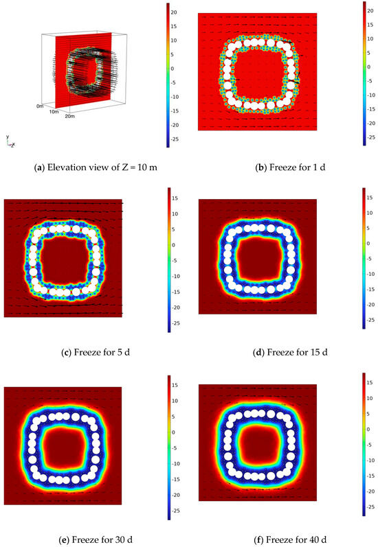
Figure 6.
Contour of the development of the frozen temperature field.
4.2. Evolution of the Freezing Curtain Under Seepage Conditions
To investigate the temporal variation in the thickness of the frozen curtain, a section at Z = 10 m was selected and analyzed. Figure 7 illustrates the evolution of −1 °C and −10 °C isotherms over time for this section. Initially, at 1 day of freezing, the −1 °C and −10 °C isotherms were confined to the vicinity of the freezing pipe, with groundwater flowing normally through the entire area surrounded by the pipe screen. By the 5th day of freezing, as the −1 °C and −10 °C isotherms started to expand, groundwater flow through the freezing zone began to decrease, with a corresponding reduction in flow rate. The −1 °C isotherm in the strong freezing zone completed its inter-circle first due to the higher density of freezing pipes in that area, indicating better freezing effectiveness. By the 11th day of freezing, the −1 °C isotherm had completed its intersection circle, at which point groundwater ceased to flow inside the permafrost curtain, and flow began to circumnavigate the −1 °C permafrost curtain. At this stage, the −10 °C isotherm completely filled the space between the pipe curtain’s steel pipes, with the outer circle of the −10 °C isotherm completing its cross-circle. By 14 days of freezing, the −10 °C isotherm had also completed its cross-circle, while the −1 °C isotherm continued to expand outward, with no groundwater flowing inside. The freezing process continued until the 40th day. The thickness of both the −1 °C and −10 °C permafrost curtains increased as the temperature continued to drop. Ultimately, the thickness of the −10 °C permafrost curtain was measured at 5.22 m, significantly surpassing the pre-established standard and meeting the excavation requirements.
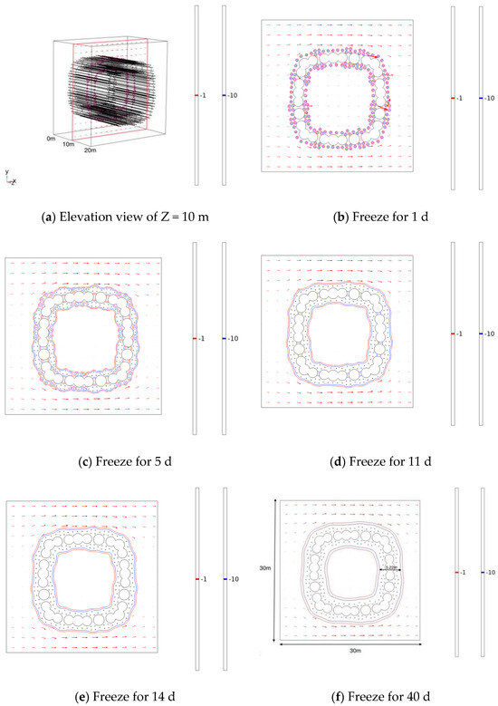
Figure 7.
Diagram of −1 °C and −10 °C isotherms.
5. Optimal Design of Freezing Scheme and Analysis of Numerical Simulation Results
The analysis of the temperature field and the thickness of the permafrost curtain reveals that the initial design for the active freezing in 40 d at −10 °C stipulates a curtain thickness of 5.22 m, which exceeds the predefined design standard of 3.5 m. Considering the economic aspect, the original design is deemed conservative, leading to significant waste. To enhance the project’s economic efficiency and ensure that the permafrost curtain thickness intersects with the −1 °C and −10 °C isotherms within the predetermined design standards, we employed the control variable method. This approach involved optimizing the design by reducing the number of freezing tubes from the original scheme. Two alternative schemes were developed, and the subsequent development of the permafrost curtain thickness following this reduction was meticulously studied. The optimal solution that not only meets the design specifications but also ensures economic viability was then selected. The optimized freezing solutions are illustrated in Table 3 and Figure 8.
Table 3.
Freezing schemes.
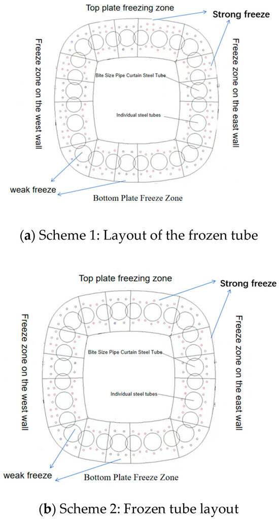
Figure 8.
Freeze Optimization Scheme Freeze Tube Layout Diagram.
5.1. Analysis of Numerical Simulation Results for Scenario 1
Through the single control variable method, other model parameters are controlled to remain unchanged, and the number of freezing pipes is reduced only on the basis of the original scheme. The Optimized Scheme 1 reduces 25 freezing pipes on the basis of the original scheme, all of which are on the inner side of the pipe curtain steel pipe, with 21 reduced in the strong freezing zone and four in the weak freezing zone. The changes in the −1 °C and −10 °C isotherms at different times are shown in Figure 9. On the 1st day of freezing, −1 °C and −10 °C isotherms only surrounded the freezing pipe. By the 5th day, the freezing pipe was completely encased in ice. By the 3rd day, the pipe curtain’s outermost −1 °C isotherm had completed its inter-circle, marking the initial formation of the frozen curtain’s outline and the onset of groundwater flow around the curtain. By the 15th day, the −1 °C isotherm had completed its inter-circle, and the entire frozen region of the pipe curtain was essentially formed. At this point, the −10 °C isotherm had completed its inter-circle in the strong freezing area and was nearly complete in the weak freezing area, with the −1 °C isotherm filling the gaps between the pipe curtain steel pipes. By the 23rd day, the −10 °C isotherm had completed its inter-circle, and there was no groundwater flow inside the permafrost curtain. There was no isotherm in the gaps between the steel pipes, indicating that the temperature in these gaps was below −10 °C, achieving the desired freezing effect. Generally, when the soil temperature reaches −10 °C, the thickness of the soil within the −10 °C isotherm is considered the effective permafrost curtain thickness. After 40 days of active freezing, the permafrost curtain was well developed, with the measured thickness of the permafrost curtain in the west side wall freezing area (upstream freezing area) being 4.34 m, in the east side wall freezing area (downstream freezing area) 4.40 m, and in the top slab freezing area 4.36 m, and in the bottom plate freezing area 4.33 m. Compared with the design standard’s limit value for the frozen soil curtain thickness of −10 °C, it was found that the frozen curtain met the requirement for soil reinforcement in the calculation result of the model for Freezing Optimized Scheme 1, ensuring the safety of construction and permitting the commencement of construction.
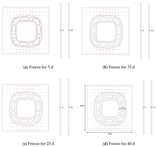
Figure 9.
Diagram of −1 °C vs. −10 °C isotherms at different times.
5.2. Analysis of Numerical Simulation Results for Scenario 2
The model’s parameters were kept constant through the single control variable method, with the reduction in freezing pipes solely based on the optimized option 1. Given that the freezing zone of the west wall is upstream, it must serve as a water barrier and thus requires a higher freezing effect. Consequently, only the freezing pipes at the top and bottom plates and the east wall freezing zone were reduced from two to one row, resulting in a total of 18 pipes being removed. The pipes in the weak freezing zones remained unchanged. Through numerical simulation, the changes in −1 °C and −10 °C isotherms at different times are illustrated in Figure 10. After 11 days of freezing, the −10 °C isotherm filled the space between the occluded and single steel pipes, indicating that the temperature outside the pipe interval was below −10 °C. The −1 °C isotherm was fully developed by day 16, and the −10 °C isotherm by day 24. After 40 days of active freezing, the permafrost curtain was well established, with the measured thickness of the curtain in the west wall freezing zone (upstream) at 4.34 m, in the east wall (downstream) at 4.17 m, in the top plate at 4.11 m, and in the bottom plate at 4.15 m. Compared to the design standard limit for the thickness of the −1 °C permafrost curtain, the optimization program was found to be very effective. Similarly, the limit value for the −10 °C curtain thickness was met, indicating that the model calculation results of the Freezing Optimized Scheme 2 satisfied the requirements for soil reinforcement, did not compromise construction safety, and could be implemented.
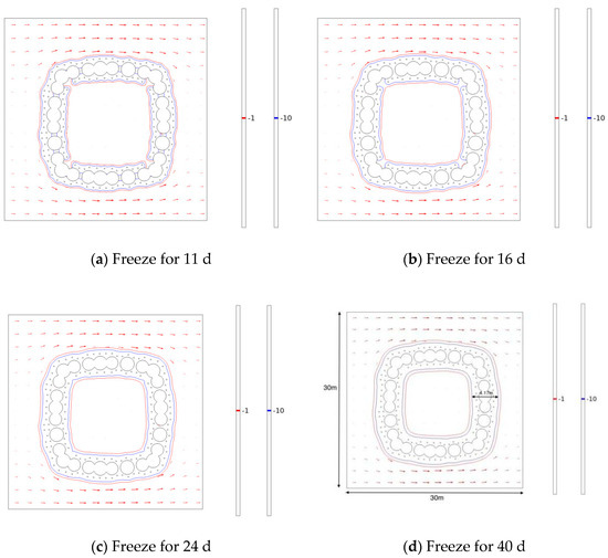
Figure 10.
Diagram of −1 °C vs. −10 °C isotherms at different times.
5.3. Comparison of the Status of Freezing Wall Development Under Different Programmes
Comparing the original scheme, as well as the Optimized Scheme 1 and Scheme 2, the statistics of the numerical simulation results for the temperature field of the three freezing schemes are presented in Table 4. As indicated in Table 4, compared to the original scheme, appropriately reducing the number of freezing pipes significantly affects the overall freezing effect. The inter-circle times for −1 °C and −10 °C isotherms are both extended, and the thicknesses of the permafrost curtain are both reduced, yet they still meet the standard values of the engineering design. Therefore, taking full consideration of the economic benefits, the number of freezing pipe arrangements can be appropriately reduced, and option 2 is recommended for freezing reinforcement.
Table 4.
Comparison of freezing conditions of different schemes.
5.4. Path Analysis
5.4.1. Path Selection
This paper explores the optimal design of pipe curtain freezing schemes under seepage conditions by reducing the freezing pipes in the strong and weak freezing zones of the original scheme. Four paths are established in the model of the three schemes, positioned upstream and downstream of the strong and weak freezing zones, to compare and analyze the differences between the two optimized schemes and the original scheme. These paths are situated in the cross-section where (Z = 10) m. Paths DJ-1 and DJ-2 are situated within the strong freezing zone. The first observation point is set at the center of the pipe curtain interval (point 0), followed by one point every 1 m interval, extending to both the inner and outer sides. The outer side is designated as positive, while the inner side is negative. Each path is equipped with a total of 7 observation points. Paths DJ-3 and DJ-4 are located in the weak freezing zone, with the first observation point set 1 m from the edge of the steel pipe on each side. Observation points are then set every 1 m interval, with each path having a total of 6 points. The path diagram is depicted in Figure 11.
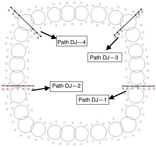
Figure 11.
Road map.
5.4.2. Analysis of Observation Points
(1) The graphs (a) and (b) of Figure 12 present the final temperatures at seven observation points for the 40th day of freezing, measured at various distances from the central point under three distinct scenarios. The plots illustrate the relationship between the final temperatures and distance. It is evident that, for all three scenarios, the temperature increases with distance from the freezing tube, indicating a reduced freezing effect. Moreover, in each scenario, the final temperatures of observation points upstream are higher than those downstream, attributed to the enhanced seepage effect upstream and the groundwater flow carrying cold from upstream to downstream. Figure 12a,b depict the temperature changes of the outer sides of steel pipes for paths DJ−1 and DJ-2 under Scenario 1 and the original scenario, as well as the inner sides of pipes for paths DJ−1 and DJ-2 under Scenario 1 and Scenario 2, and the outer sides of pipes for paths DJ-3 and DJ-4 under all three scenarios. These observations show minimal temperature changes and nearly identical curves, reflecting the lack of optimization in the number of freezing pipes at these locations. Under Scenario 2, the optimization of the number of freezing tubes on the outer side of path DJ−1 results in higher final temperatures compared to the original scenario, with the temperature difference at the most distant observation points being only 6 °C. Similarly, the final temperatures of paths DJ-3 and DJ-4 under Scenario 1 and Scenario 2 are higher than those under the original scenario, attributable to the optimization of the number of freezing tubes on the inner side, with a temperature difference of only 8 °C between the optimized scenarios and the original scenario, which meets the design criteria.
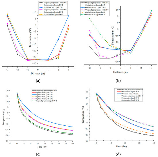
Figure 12.
Path analysis diagram. (a) Frozen final temperature map of the path observation point at the strong freeze zone. (b) Map of the frozen final temperature of the path observation point at the weak freeze zone. (c) Map of temperature change of path observation points at strong freezing areas. (d) Temperature change map of the path observation point at the weak frozen area.
(2) The figure in Figure 12 presents the temperature changes over time for the three programs, based on the selection of four paths in both the upstream and downstream strong and weak freezing zones. The weighted average daily temperatures of the seven observation points on each path during the active freezing period for 40 days were measured. The plots in Figure 12c,d indicate that during the initial 10 days of freezing and cooling, the cooling rates for the four paths under the three schemes were faster, and then they gradually leveled off after 10 days. This is attributed to the higher cooling rate of the brine cooling scheme during the first 10 days. From the average temperature change curve of the four paths under the original scheme, it can be inferred that the cooling effect in the downstream is superior due to the influence of the direction of groundwater seepage, which transports cold to the downstream area. Under Optimized Scheme 1 and Scheme 2, the cooling curves for paths DJ-2, DJ-3, and DJ-4 are essentially the same, suggesting that there is no significant difference in the average temperatures of the same paths under the different schemes. This is because the freezing areas where these paths are located were not optimized, nor was the number of freezing pipes. Figure 12c reveals a notable difference in the cooling curves for path DJ−1 under Optimized Scheme 1 and Scheme 2, primarily due to the optimization of the number of freezing pipes in the downstream strong freezing zone. Ultimately, the average temperature of the original scheme stabilizes at −19.63 °C, while the average temperature of Optimized Scheme 2 stabilizes at −12.65 °C, despite a difference of approximately 7 °C. However, the temperature of Optimized Scheme 2 stabilizes at about −12.65 °C, which meets the design standard: the average temperature of the strong freezing zone is ≤ −10 °C.
(3) The temperature field maps, isotherm maps, and path cooling curves provide a visual representation of the freezing temperature field’s evolution. Yet, they do not quantitatively depict the development of the frozen curtain thickness, an essential indicator of the frozen curtain’s integrity. To quantitatively assess the frozen curtain’s development, the thickness of the frozen wall must be measured. To clearly compare the freezing wall’s development under the three schemes, the thickness of the freezing wall at the downstream strong freezing zone (path DJ−1) was selected as the basis for this study. As shown in Figure 13, the curve diagram of the freezing wall thickness with freezing time in the strong freezing zone of path DJ−1 indicates that the freezing wall begins to form thickness from the 3rd day of freezing. Initially, the thickness of the freezing wall for the three schemes develops rapidly within the first 10 days, a result of the larger cooling amplitude of the brine cooling scheme during this period. In the original program, after the 10th day, the thickness of the frozen wall was impeded by the steel pipe, leading to a gradual slowdown in its development. By the end of 40 days of active freezing, the thickness of the frozen wall reached 2.52 m. After the 10th day of freezing, Optimization 1 and Optimization 2 developed more slowly due to the influence of groundwater flow, which slowed the development of the frozen wall. When the isotherms intersected at 23 days, the flow of groundwater was impeded, and the development of the frozen wall thickness accelerated compared to before. The freezing wall thickness of Optimized Plan 1 reached 2.2 m, and that of Optimized Plan 2 reached 2.08 m, both of which met the design criteria.
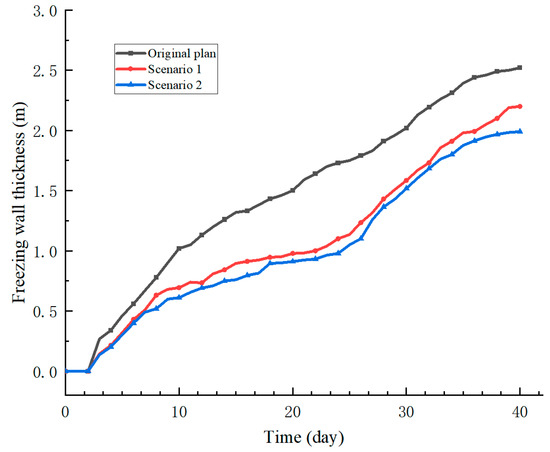
Figure 13.
Variation of frozen wall thickness.
6. Conclusions
This paper presents a study on the Sanya Estuary Passage submarine pipeline curtain freezing tunnel project, employing COMSOL software to develop a three-dimensional numerical transient model for a detailed analysis of the pipe curtain freezing temperature field. By refining the original freezing scheme based on the results of the temperature field analysis, several conclusions have been drawn:
- (1)
- The number of freezing pipes in the strong freezing zone exceeds that in the weak freezing zone, and the average temperature in the strong freezing zone is lower than that in the weak freezing zone, indicating that the number of freezing pipes significantly influences the freezing effect. When the freezing curtain is essentially formed, it is evident that the groundwater flow lines bypass the freezing curtain, suggesting that the freezing curtain acts as a barrier to water flow. Due to the more pronounced seepage flow upstream compared to downstream during the active freezing period (40 days), groundwater flow carries cold from upstream freezing pipes to the downstream area, resulting in a more pronounced freezing effect downstream than upstream. Consequently, optimization of treatment can be applied to the downstream freezing pipes.
- (2)
- The original scheme, with a 10 °C isotherm, completes all inter-circle operations in 14 days. The Optimized Scheme 1 is 7 days slower than the original scheme, while Optimized Scheme 2 is 10 days slower. However, all schemes are within the predetermined design standard of 25 days, thus meeting the design requirements.
- (3)
- The original plan calls for permafrost curtains with thicknesses of 5.22 m, 5.05 m, 5.16 m, and 4.67 m in the southeast and northwest. In contrast, the optimized plan reduces these thicknesses to 4.4 m, 4.36 m, 4.34 m, and 4.43 m in the same areas. The optimized plan further reduces the thicknesses to 4.17 m, 4.11 m, 4.34 m, and 4.15 m, with the greatest reduction observed in the east wall (downstream), where the difference between the optimized plan 2 and the original plan 1 is 1.05 m, and between optimized plan 1 and optimized plan 2 is 0.23 m. The most significant reduction in thickness is observed in the east wall (downstream), where the difference between Optimized Scheme 2 and the original plan is 1.05 m, and between Optimized Scheme 1 and Optimized Scheme 2 is 0.23 m. The average thickness of the permafrost curtain on the four sides of Optimized Scheme 2 is 4.18 m, significantly exceeding the design standard of 3.5 m.
- (4)
- The freezing effect of permafrost curtains under the arrangement of freezing pipes in the original freezing program is good, and it is safe and feasible in the actual construction, but the number of freezing pipes is used too much, which will improve the economic cost of construction. Therefore, through the comparison and analysis of the two optimization schemes, under the premise of conforming to the design standard, the number of freezing pipes is reduced moderately. However, it will make the freezing curtain inter-circle longer, and the thickness of the freezing curtain will be reduced, but all of them satisfy the design requirements. The comprehensive comparison concludes that Optimized Scheme 2 is preferable.
Reducing the use of freezing pipes and improving the efficiency of the freezing method through optimization is important for future underground applications. By optimizing the layout of freezing pipes, construction costs can be significantly reduced, construction time shortened, and environmental impact reduced. In addition, as technology advances, it is expected that future freezing methods will be more efficient, environmentally friendly and applicable, providing strong support for the development of urban underground space and infrastructure construction.
Author Contributions
Conceptualization, T.Y. and J.H.; methodology, T.Y. and J.H. and Y.W. (Yongwei Wang); validation, J.H., H.G. and S.Z.; data curation, T.Y.; writing—original draft preparation, T.Y. and J.H.; writing—review and editing, J.H., H.G. and T.Y.; funding acquisition, J.H. and Y.W. (Ying Wang). All authors have read and agreed to the published version of the manuscript.
Funding
High Technology Direction Project of the Key Research and Development Science and Technology of Hainan Province, China (Grant No. ZDYF2024GXJS001); Hainan University 2022 Collaborative Innovation Centre Research Projects (XTCX2022STB09); Key Research and Development Projects of Haikou Science and Technology Plan for the Year 2023 (2023-012); Hainan University Horizontal Research Project ‘Research on Safety Construction Guarantee Technology for Tunnel and Very Large Deep Foundation Pit with Long Distance Pipe Curtain Freezing Method in Shallow Overburden under Sea Environment’ (HD-KYH-2022405); The Hainan Provincial Innovation Foundation for Postgraduates (Qhyb2023−117).
Institutional Review Board Statement
Not applicable.
Informed Consent Statement
Not applicable.
Data Availability Statement
The original contributions presented in the study are included in the article, further inquiries can be directed to the corresponding author.
Conflicts of Interest
The authors declare no conflicts of interest.
References
- Yang, H.Y.; Jiang, Y.; Li, Z.; Gao, J.J.; Wang, B.C. Study on development strategies for integrated management of underground space development. Chin. Acad. Eng. Sci. 2021, 23, 126–136. [Google Scholar] [CrossRef]
- Pan, W.Q. Monitoring and Analysis of Ground Subsidence for Pipe Jacking Construction of Pipe Curtain Group in Soft Soil Area. Chin. J. Geotech. Eng. 2019, 41 (Suppl. S1), 201–204. [Google Scholar]
- Tang, L. Application of Horizontal Artificial Freezing Technology in Water-Rich Shallow Buried Undercover Tunnels. Road Traffic Technol. 2013, 1, 111–115. [Google Scholar]
- Cai, H.B.; Cheng, Y.; Peng, L.M.; Yao, Z.S.; Rong, C.X. Modelling of Horizontal Freezing Displacement Field in a Two-Lane Metro Tunnel. J. Rock Mech. Eng. 2009, 28, 2088–2095. [Google Scholar]
- Shi, C.H. Unified Prediction Theory and Application of Ground Deformation in Urban Tunnel Construction. J. Rock Mech. Eng. 2008, 27, 1082. [Google Scholar]
- Li, F.Z. Development status and trend of subway freezing technology. Well Constr. Technol. 2020, 41, 33–42. [Google Scholar]
- Liu, Q.Q.; Cai, G.Q.; Zhou, C.X.; Yang, R.; Li, J. Thermo-hydro-mechanical coupled model of unsaturated frozen soil considering frost heave and thaw settlement. Cold Reg. Sci. Technol. 2024, 217, 104026. [Google Scholar] [CrossRef]
- Wu, Y.; Zhai, E.; Zhang, X.; Wang, G. A study on frost heave and thaw settlement of soil subjected to cyclic freeze-thaw conditions based on hydro-thermal-mechanical coupling analysis. Cold Reg. Sci. Technol. 2021, 188, 103296. [Google Scholar] [CrossRef]
- Zhang, Y.; Michalowski, L.R. Thermal-Hydro-Mechanical Analysis of Frost Heave and Thaw Settlement. J. Geotech. Geoenviron. Eng. 2015, 141, 04015027. [Google Scholar] [CrossRef]
- Sinnathamby, G.; Gustavsson, H.; Korkiala, T.L.; Pérez, C.C.; Koskinen, M. Frost Heave and Thaw Settlement Estimation of a Frozen Ground. In Proceedings of the 15th Pan-American Conference on Soil Mechanics and Geotechnical Engineering, Buenos Aires, Argentina, 15–18 November 2015; pp. 891–898. [Google Scholar]
- Zhou, J.Q.; Wu, X.Y.; Zhao, Y.L. Research on the Development Status and Application of Pipe Curtain Method Construction Technology. J. Zhejiang Jiaotong Vocat. Tech. Coll. 2024, 25, 46–51. [Google Scholar]
- Hu, X.; Wu, Y.; Li, X. A field study on the freezing characteristics of freeze-sealing pipe roof used in ultra-shallow buried tunnel. Appl. Sci. 2019, 9, 1532. [Google Scholar] [CrossRef]
- Hong, Z.; Hu, X.; Fang, T. Analytical solution to steady-state temperature field of Freeze-Sealing Pipe Roof applied to Gongbei tunnel considering operation of limiting tubes. Tunn. Undergr. Space Technol. 2020, 105, 103571. [Google Scholar] [CrossRef]
- Duan, Y.; Rong, C.X.; Cheng, H.; Cai, H.B.; Jie, D.Z. Modeltest of pipe curtain freezing temperature field with different pipe jacking combinations. Glacial Permafr. 2020, 42, 479–490. [Google Scholar]
- Lu, Y.Y.; Zhang, H.; Wei, L.H.; Huang, X.J. Wait. Numerical simulation of temperature field during freezing process by pipe curtain freezing method. Railw. Constr. 2017, 57, 52–54+58. [Google Scholar]
- Hu, X.D.; Li, X.Y.; Wu, Y.H. Experimental study on the effect of freezing and sealingwater between pipes by pipe curtain freezing method in Gongbei tunnel. Chin. J. Geotech. Eng. 2019, 41, 2207–2214. [Google Scholar]
- Zhang, J.; Wu, S.Y.; Cheng, Y.; Liu, J.G. Long-distance curve pipe curtain freezing shallow buried underground excavation tunnel project-GongbeiTunnel of Hong Kong-Zhuhai-Macao Bridge. Tunn. Constr. Chin. Engl. 2019, 39, 164–171. [Google Scholar]
- Long, W.; Rong, C.X.; Duan, Y.; Guo, K. Numerical calculation of temperature field by freezing method of pipe curtain in Gongbei tunnel. Coal Geol. Explor. 2020, 48, 160−168. [Google Scholar]
- Hu, X.D.; Deng, S.J.; Ren, H. In situ test study on f reezing scheme of freeze-sealing pipe roof applied to the gongbei tunnel in the hong kong-zhuhai-macau bridge. Appl. Sci. 2017, 7, 27. [Google Scholar] [CrossRef]
- Duan, Y.; Rong, C.X.; Cheng, H.; Cai, H.B.; Long, W. Freezing temperature field of FSPR under different pipe configurations: A case study in gongbei tunnel, China. Adv. Civ. Eng. 2021. [Google Scholar] [CrossRef]
- Long, W.; Rong, C.X.; Shi, H.; Huang, S.Q.; Wang, B.; Duan, Y.; Wang, Z.; Shi, X.; Ma, H.C. Temporal and spatial evolution law of the freezing temperature field of water-rich sandy soil under groundwater seepage: A case study. Processes 2022, 10, 2307. [Google Scholar] [CrossRef]
- Pang, C.Q.; Cai, H.B.; Hong, R.B.; Li, M.K.; Yang, Z. Evolution law of three-dimensional non-uniform temperature field of tunnel construction using local horizontal freezing technique. Appl. Sci. 2022, 12, 8093. [Google Scholar] [CrossRef]
- Li, M.; Cai, H.; Liu, Z.; Pang, C.; Hong, R. Research on frost heaving distribution of seepage stratum in tunnel construction using horizontal freezing technique. Appl. Sci. 2022, 12, 11696. [Google Scholar] [CrossRef]
- Yao, Z.; Cai, H.; Xue, W.; Wang, X.; Wang, Z. Numerical simulation and measurement analysis of the temperature field of artificial freezing shaft sinking in Cretaceous strata. AIP Adv. 2019, 9, 025209. [Google Scholar] [CrossRef]
- Li, Z.; Chen, J.; Sugimoto, M.; Mao, C. Thermal behavior in cross-passage construction during artificial ground freezing: Case of Harbin metro line. J. Cold Reg. Eng. 2020, 34, 05020002. [Google Scholar] [CrossRef]
- Gao, G.; Guo, W.; Ren, Y. Coupled modelling of artificial freezing along clay-sand interface under seepage flow conditions. Cold Reg. Sci. Technol. 2023, 211, 103865. [Google Scholar] [CrossRef]
- Hu, J.; Liu, Y. Effect of heating limit tube on the thickness of frozen soil curtain. For. Eng. 2016, 32, 69–74. [Google Scholar]
- Wu, Y.W. Research on the Evolution of Construction Temperature Field of Freezing Method of Dongbin Section of Nanning Metro; Hainan University: Haikou, China, 2019. [Google Scholar]
- Liu, W.B. Research on Freezing and Reinforcement Technology of Large-Diameter Shield Tunneling in Heyan Road Cross-River Channel in Nanjing; Hainan University: Haikou, China, 2021. [Google Scholar]
Disclaimer/Publisher’s Note: The statements, opinions and data contained in all publications are solely those of the individual author(s) and contributor(s) and not of MDPI and/or the editor(s). MDPI and/or the editor(s) disclaim responsibility for any injury to people or property resulting from any ideas, methods, instructions or products referred to in the content. |
© 2024 by the authors. Licensee MDPI, Basel, Switzerland. This article is an open access article distributed under the terms and conditions of the Creative Commons Attribution (CC BY) license (https://creativecommons.org/licenses/by/4.0/).