Enhancing Word Embeddings for Improved Semantic Alignment

Abstract

This study introduces a method for the improvement of word vectors, addressing the limitations of traditional approaches like Word2Vec or GloVe through introducing into embeddings richer semantic properties. Our approach leverages supervised learning methods, with shifts in vectors in the representation space enhancing the quality of word embeddings. This ensures better alignment with semantic reference resources, such as WordNet. The effectiveness of the method has been demonstrated through the application of modified embeddings to text classification and clustering. We also show how our method influences document class distributions, visualized through PCA projections. By comparing our results with state-of-the-art approaches and achieving better accuracy, we confirm the effectiveness of the proposed method. The results underscore the potential of adaptive embeddings to improve both the accuracy and efficiency of semantic analysis across a range of NLP.

1. Introduction

To effectively process text, it is necessary to represent it numerically, which allows computers to analyze a document’s content. Creating an appropriate representation of a text is fundamental to achieving good results from machine learning algorithms. Traditional approaches to text representation treat documents as points in a high-dimensional space, where each axis corresponds to a word in the vocabulary. In this model, documents are represented as vectors with coefficients indicating the frequency of each word in the text (e.g., using the TF-IDF in a vector space model (VSM) [1]).

But this approach is limited by its inability to capture the semantics of words. When using word-based representations in a VSM, we cannot distinguish between synonyms (words with similar meanings but different forms) and homonyms (words with the same form but different meanings). For example, the words “car” and “automobile” may be treated as completely different entities in word space, even though they have the same meaning. Such information can be provided to the NLP system by an external database. A good example that provides such information is the WordNet dictionary [2], which is organized in the form of a semantic network that contains relationships between synsets that describe groups of words that have the same meaning [3]. Other approaches may include interactions with humans that enrich the vector representations with semantic features [4]. Nevertheless, in the context of NLP, word embeddings have a lot of potential compared to the use of semantic networks. One advantage is their ability to perform classical algebraic operations on vectors, such as addition or multiplication.

To address the problem of semantic word representation, an extension of the VSM was introduced using a method known as word embeddings. In this model, each word is represented as a vector in a multidimensional space, and the similarity between vectors reflects the semantic similarity between words. Models such as Word2Vec [5], GloVe [6], FastText [7] and others learn word representations in an unsupervised manner. The training is based on the context in which words appear in a text corpus, which allows some elementary relationships between them to be captured [8]. In the research presented in our paper, we refer to these embeddings as original embeddings (OE), which were used in the experiments as GloVe vectors.

Using vector-based representations, geometric operations become possible, enabling basic semantic inference. A classic example, proposed by Tomas Mikolov [5], is the operation king-man + woman = queen, which demonstrates how vectors can capture hierarchical relationships between words [9]. These operations enhance the modeling of language dependencies, enabling more advanced tasks like machine translation, semantic searches, and sentiment analysis.

Our study aims to explore methods for creating semantic word embeddings, namely embeddings that carry precise meanings with a strong reference to WordNet. We present methods for building improved word embeddings based on semi-supervised techniques. In our experiments, we refer to these embeddings as neural embeddings (NE). After applying the alignment we refer to them as Fine-tuned Embeddings (FE). Our approach extends the method proposed in [10], modifying word vectors so that geometric operations on them correspond to fundamental semantic relationships. We call this method geometrical embeddings (GE).

The word embeddings generated by our approach have been evaluated in terms of their usefulness for text classification, clustering, and the analysis of class distribution in the embedded representation space.

The rest of this paper is organized as follows: Section 2 describes various methods for creating word embeddings, both supervised and unsupervised. Section 3 presents our approach, including the dataset, the preprocessing methods and techniques used to create semantic word embeddings, and the evaluation methodology. Section 4 presents the experimental results. Section 5 contains a brief discussion of the overall findings, followed by Section 6 which outlines potential applications and future research directions.

2. Related Works

Word embeddings, also known as distributed word representations, are typically created using unsupervised methods. Their popularity stems from the simplicity of the training process, as only a large corpus of text is required. The embedding vectors are first constructed from sparse representations and then mapped to a lower-dimensional space, producing vectors that correspond to specific words. To provide context for our research, we briefly describe the most popular approaches to building word embeddings.

After the pioneering work of Bengio et al. on neural language models [11], research on word embeddings stalled due to limitations in computational power and algorithms being insufficient for training large vocabularies. However, in 2008, Collobert and Weston showed that word embeddings trained on sufficiently large datasets capture both syntactic and semantic properties, improving performance in subsequent tasks. In 2011, they introduced SENNA embeddings [12], based on probabilistic models that allow for the creation of word vectors. For each training iteration, an n-gram was used by combining the embeddings of all n words. The model then modified the n-gram by replacing the middle word with a random word from the vocabulary. It was trained to recognize that the intact n-gram was more meaningful than the modified (broken) one, using a hinge loss function. Shortly thereafter, Turian et al. replicated this method, but instead of replacing the middle word, they replaced the last word [13], achieving slightly better results.

These embeddings have been tested on a number of NLP tasks, including Named Entity Recognition (NER) [14], Part of Speech (POS) [15], Chunking (CHK) [16], Syntactic Parsing (PSG) [17], and Semantic Role Labeling (SRL) [18]. This approach has shown improvement in a wide number of tasks [19] and is computationally efficient, using only 200 MB of RAM.

Word2vec is a set of models introduced by Mikolov et al. [5] that focuses on word similarity. Words with similar meanings should have similar vectors, while words with different vectors do not have similar meanings. Considering the two sentences “They like watching TV ” and “They enjoy watching TV”, we can conclude that the words like and enjoy are very similar, although not identical. Primitive methods like one-hot encoding would not be able to capture the similarity between them and would treat them as separate entities, so the distance between the words {like, TV} would be the same as the distance between {like, enjoy}. In the case of word2vec, the distance between {like, TV} would be greater than the distance between {like, enjoy}. Word2vec allows one to perform basic algebraic operations on vectors, such as addition and subtraction.

The GloVe algorithm [6] integrates word co-occurrence statistics to determine the semantic associations between words in the corpus, which is somewhat the opposite to Word2vec—which depends only on local features in words. GloVe implements the global matrix factorization technique, which uses a matrix to encode the presence or absence of word occurrences. Word2vec is commonly known as neural word embeddings; hence, it is a feedforward neural network model, whereas GloVe is commonly known as a count-based model, also called a log-bilinear model. By analyzing how frequently words co-occur in a corpus, GloVe captures the relationships between words. The co-occurrence likelihood can encode semantic significance, which helps improve performance on tasks like the word analogy problem.

FastText is another method developed by Joulin et al. [20] and further improved [21] by introducing an extension of the continuous skipgram model. In this approach, the concept of word embedding differs from Word2Vec or GloVe, where words are represented by vectors. Instead, word representation is based on a bag of character n-grams, with each vector corresponding to a single character n-gram. By summing the vectors of the corresponding n-grams, we obtain the full word embedding.

As the name suggests, this method is fast. In addition, since the words are represented as a sum of n-grams, it is possible to represent words that were not previously added to the dictionary, which increases the accuracy of the results [7,22]. The authors of this approach have also proposed a compact version of fastText, which, due to quantization, maintains an appropriate balance between model accuracy and memory consumption [23].

Peters et al. [24] introduced the ELMo embedding method, which uses a bidirectional language model (biLM) to derive word representations based on the full context of a sentence. Unlike traditional word embeddings, which map each token to a single dense vector, ELMo computes representations through three layers of a language model. The first layer is a Convolutional Neural Network (CNN), which produces a non-contextualized word representation based on the word’s characters. This is followed by two bidirectional Long Short-Term Memory (LSTM) layers that incorporate the context of the entire sentence.

By design, ELMo is an unsupervised method, though it can be applied in supervised settings by passing pretrained vectors into models like classifiers [25]. When learning a word’s meaning, ELMo uses a bidirectional RNN [26], which incorporates both preceding and subsequent context [24]. The language model learns to predict the likelihood of the next token based on the history, with the input being a sequence of n tokens.

Bidirectional Encoder Representations of Transformers, often referred to as BERT [27], is a transformer-based architecture. Transformers were first introduced relatively recently, in 2017 [28]. This architecture does not rely on recursion, as previous state-of-the-art systems (such as LSTM or ELMo) did, significantly speeding up training time. This is because sentences are processed in parallel rather than sequentially, word by word. A key unit, self-attention, was also introduced to measure the similarity between words in a sentence. Instead of recursion, positional embeddings were created to store information about the position of a word/token in a sentence.

BERT was designed to eliminate the need for decoders. It introduced the concept of masked language modeling, where 15% of the words in the input are randomly masked and predicted using positional embeddings. Since predicting a masked token only requires the surrounding tokens in the sentence, no decoder is needed. This architecture set a new standard, achieving state-of-the-art results in tasks like question answering. However, the model’s complexity leads to slow convergence [27].

Beringer et al. [10] proposed an approach to represent unambiguous words based on their meaning in the context [29]. In this method, word vector representations are adjusted according to polysemy: vectors of synonyms are brought closer together in the representation space, while vectors of homonyms are separated. The supervised iterative optimization process leads to the creation of vectors that offer more accurate representations compared to traditional approaches like word2vec or GloVe.

Pretrained models can be used across a wide range of applications. For instance, the developers of Google’s Word2Vec trained their model on unstructured data from Google News [30], while the team at Stanford used data from Wikipedia, Twitter, and web crawling for GloVe [31]. Competing with these pretrained solutions is challenging; instead, it is often more effective to leverage them. For example, Al-Khatib and El-Beltagy applied the fine-tuning of pretrained vectors for sentiment analysis and emotion detection tasks [32].

To further leverage the power of pretrained embeddings, Dingwall and Potts developed the Mittens tool for fine-tuning GloVe embeddings [33]. The main goal is to enrich word vectors with domain-specific knowledge, using either labeled or unlabeled specialized data. Mittens transforms the original GloVe goal into a retrofitting model by adding a penalty for the squared Euclidean distance between the newly learned embeddings and the pretrained ones. It is important to note that Mittens adapts pretrained embeddings to domain-specific contexts, rather than explicitly incorporating semantics to build semantic word embeddings.

3. Material and Methods

In this section, we describe our method for building word embeddings that incorporate elementary semantic information. We begin by detailing the dedicated dataset used in the experiments. Next, we explain our method, which modifies the hidden layer of a neural network initialized with pretrained embeddings. We then describe the fine-tuning process, which is based on vector shifts. The final subsection outlines the methodology used to evaluate the proposed approach.

3.1. Dataset

For our experiments, we constructed a custom dataset consisting of four categories: animal, meal, vehicle, and technology. Each category contains six to seven keywords, for a total of 25 words.

We also collected 250 sentences for each keyword (6250 in total) using web scraping from various online sources, including most English dictionaries. The sentences contain no more than one occurrence of the specified keyword.

The words defining each category were selected such that the boundaries between categories were fuzzy. For instance, the categories vehicle and technology, or meal and animal, overlap to some extent. Additionally, some keywords were chosen that could belong to more than one category but were deliberately grouped into one. An example is the word fish, which can refer to both a food and an animal. This was carried out intentionally to make it more difficult to classify the text and highlight the contribution our word embeddings aim to address.

To prepare and transform raw data into useful formats, preprocessing is essential for developing or modifying word embeddings [34,35]. The following steps were taken to prepare the data for further modeling:

1.

Change all letters to lowercase;

2.

Remove all non-alphabetic characters (punctuation, symbols, and numbers);

3.

Remove unnecessary whitespace characters: duplicated spaces, tabs, or leading spaces at the beginning of a sentence;

4.

Remove selected stop words using a function from the Gensim library: articles, pronouns, and other words that will not benefit the creation of embeddings;

5.

Tokenize, i.e., divide the sentence into words (tokens);

6.

Lemmatize, bringing variations of words into a common form, allowing them to be treated as the same word [36]. For example, the word cats would be transformed into cat, and went would be transformed into go.

3.2. Method of Semantic Word Embedding Creation

In this section, we describe in detail our method for improving word embeddings. This process involves three steps: training a neural network to obtain an embedding layer, tuning the embeddings, and shifting the embeddings to incorporate specific geometric properties.

3.2.1. Embedding Layer Training

For building word embeddings in the neural network, we use a hidden layer with initial weights set to pretrained embeddings. In our tests, the architectures with fewer layers performed best, likely due to the small gradient in the initial layers. As the number of layers increased, the initial layers were updated less effectively during backpropagation, causing the embedding layer to change too slowly to produce strongly semantically related word embeddings. As a result, we used a smaller network for the final experiments.

The algorithm for creating semantic embeddings using a neural network layer is as follows:

1.

Load the pretrained embeddings.

2.

Preprocess the input data.

3.

Separate a portion of the training data to create a validation set. In our approach, the validation set was 20% of the training data.

Next, the initial word vectors were combined with the pretrained embedding data. To achieve this, an embedding matrix was created, where the row at index i corresponds to the pretrained embedding of the word at index i in the vectorizer.

4.

Load the embedding matrix into the embedding layer of the neural network, initializing it with pretrained word embeddings as weights.

5.

Create a neural network-based embedding layer.

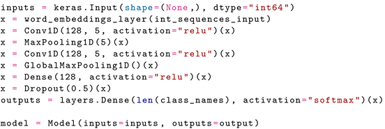
In our experiments, we tested several architectures. The one that worked best was a CNN with the following configuration.

6.

Train the model using the prepared data.

7.

Map the data into words in vocabulary embeddings created in hidden layer weights.

8.

Save the newly created embeddings in a pickle format.

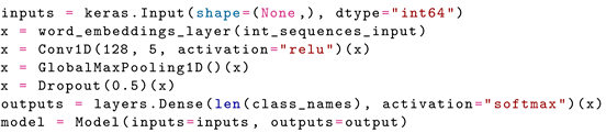
After testing several network architectures, we found that the models with fewer layers performed best. This is likely due to the small gradient in the initial layers. As the number of layers increases, the initial layers are less effectively updated during backpropagation, causing the embedding layer to change too slowly to produce strongly semantic word embeddings. For this reason, a smaller network was used for the final experiments, with the following configuration.

3.2.2. Fine-Tuning of Pretrained Word Embeddings

This step uses word embeddings created in a self-supervised manner by fine-tuning pretrained embeddings.

The entire process for training embeddings is encapsulated in the following steps:

1.

Load the pretrained embeddings. The algorithm uses GloVe embeddings as input, so the embeddings need to be converted into a dictionary.

2.

Preprocess the input data (described in Section 3.1).

3.

Prepare a co-occurrence matrix of words using the GloVe mechanism.

4.

Train the model using the function provided by Mittens for fine-tuning GloVe embeddings [33].

5.

Save the newly created embeddings in a pickle format.

3.2.3. Embedding Shifts

The goal of this step is to adjust word vectors in the representation space, enabling geometric operations on pretrained embeddings that incorporate semantics from the WordNet network. To achieve this, we used the implementation by Beringer et al., available on GitHub [37]. However, to adapt the code to the planned experiments, the following modifications were introduced:

• Modification of the pretrained embeddings: Since Beringer et al. originally used embeddings from the SpaCy library as a base [38], even though they also used the GloVe method for training, the data they used differed. Therefore, it was necessary to modify how the vectors were loaded. While SpaCy provides a dedicated function for this task, it had to be replaced with an alternative.
• Manual splitting of the training set into two smaller sets, one for training (60%) and one for validation (40%), aimed at proper hyperparameter selection.
• Adapting other features: Beringer et al. created embeddings by combining the embedding of a word and the embedding of the meaning of that word, for example, the word tree and its meaning forest, or tree (structure). They called them keyword embeddings. In the case of the experiment conducted in this thesis, the embeddings of the word and the category were combined, like cat and animal, or airplane (technology). An embedding created in this way is called a keyword–category embedding. The term keyword embedding is used to describe any word contained in categories, such as cat, dog, etc. The term category embedding describes the embedding of a specific category word, namely animal, meal, technology, or vehicle.
• Adding hyperparameter selection optimization:

Finally, for the sake of clarity, the algorithm design was as follows:

1.

Upload or recreate non-optimized keyword–category embeddings. For each keyword in the dataset and its corresponding category, we created an embedding, as shown in Equation (1), which included both sample objects and category items:

$$k{c}_{fish\left(animal\right)}=e(fish,animal)={\displaystyle \frac{e\left(fish\right)+e\left(animal\right)}{2}}$$

(1)

2.

Load and preprocess the texts used to train the model.

3.

For each epoch:

3.1.

For each sentence in the training set:

3.1.1.

Calculate the context embedding. The context itself is the set of words surrounding the keyword, as well as the keyword itself. We create the context embedding by averaging the embeddings of all the words that make up that context.

3.1.2.

Measure the cosine distance between the computed context embedding and all category embeddings. In this way, we select the closest category embedding and check whether it is a correct or incorrect match.

3.1.3.

Update keyword–category embeddings. The algorithm moves the keyword–category embedding closer to the context embedding if the selected category embedding turns out to be correct. If not, the algorithm moves the keyword–category embedding away from the context embedding. The alpha ($\alpha$) and beta ($\beta$) coefficients determine how much we manipulate the vectors.

4.

Save the newly modified keyword–category embeddings in the pickle format. The pickle module is a method for serializing and deserializing objects, developed in the Python programming language [39].

The top-k accuracy on the validation set was used as a measure of the quality of the embeddings to be used in selecting appropriate hyperparameters and selecting the best embeddings. This is a metric that determines whether the correct category is in the top k categories, where the input data are context embeddings from the validation set. Due to the small number of categories (4 in total), it was decided to evaluate the quality of the embeddings using the top-1 accuracy. Finally, a random search yielded the optimal hyperparameters.

3.3. Semantic Word Embedding Evaluation

We performed the evaluation of our method for building the word embeddings using two applications. We tested how they influence the quality of the classification, and we measured their distribution and plotted them using PCA projections. We also evaluated how the introduction of the embeddings influences the unsupervised processing of the data.

3.3.1. Text Classification

The first test for the newly created semantic word embeddings was based on a prediction of the category from the sentence. This can be carried out in many ways, for example, by using the embeddings as a layer in a deep neural network. Initially, however, it would be better to test the capabilities of the embeddings themselves without further training on the new architecture. Thus, we used a method based on measuring the distance between embeddings. In this case, our approach consisted of the following steps:

1.

For each sentence in the training set:

1.1.

Preprocess the sentence.

1.2.

Convert the words from the sentence into word embeddings.

1.3.

Calculate the mean embedding from all the embeddings in the sentence.

1.4.

Calculate the cosine distance between the mean sentence embedding and all category embeddings based on Equation (2):

$$distance(\overline{e},c)=cos(\overline{e},c)={\displaystyle \frac{\overline{e}·c}{∥\overline{e}∥∥c∥}}$$

(2)

where $\overline{e}$ is the mean sentence embedding and c is the category embedding.

1.5.

Select the assigned category by taking the category embedding with the smallest distance from the sentence embedding.

2.

Calculate the accuracy score by taking the predictions for all sentences based on Equation (3):

$$Accuracy={\displaystyle \frac{Numberofcorrectpredictions}{Totalnumberofpredictions}}$$

(3)

In addition, in modern research, weighted embeddings are typically used to improve the quality of the prediction [40,41]. Latent semantic analysis uses a term–document matrix that takes into account the frequency of a term’s occurrence. This is accomplished by using the TF-IDF weighting schema, which is used to measure the importance of a term by its frequency of occurrence in a document.

To fully see the potential of word embeddings in classification, it is beneficial to combine them with a separate classification model, distinct from the DNN used to create the embeddings. We chose a KNN and Random Forest [42], which are non-neural classifiers, to avoid introducing any bias into the results. It should be noted that for the evaluation of the embeddings, any other classifier can be used.

3.3.2. Separability and Spatial Distribution

To measure the quality of the semantic word embeddings, we checked their spatial distribution by performing two tests. The first was an empirical test aimed at reducing the dimensionality of the embeddings and visualizing them in two-dimensional space using the Principal Component Analysis (PCA) method, which transforms multivariate data into a smaller number of representative variables, preserving as much accuracy as possible. In other words, the goal is to achieve a trade-off between the simplicity of the representation and accuracy [43].

Still considering the quality of the semantic word embeddings, we computed the relevant metrics, which prove the separability of the classes, as well as the correct distribution of the vectors in space. In view of this, we used the mean distance of all the keywords to their respective category words. The purpose of checking these distances is to test whether the average embedding of keywords in a given category yields a vector that is close to the category vector, evaluated based on Equation (4), with sample objects from the same semantic category.

$${\displaystyle \frac{e\left(computer\right)+e\left(CPU\right)+e\left(keyboard\right)+e\left(monitor\right)+e\left(TV\right)+e\left(phone\right)}{6}}\approx e\left(technology\right)$$

(4)

The formula for calculating the average distance of keyword embeddings from their category embeddings is based on Equation (5).

$$meanDistanceToCategory(c,C)={\displaystyle \frac{1}{\left|C\right|}}\sum _{k\in C}cos(c,k)={\displaystyle \frac{1}{\left|C\right|}}\sum _{k\in K}{\displaystyle \frac{c·k}{∥c∥∥k∥}}$$

(5)

where

• c is a category embedding;
• C is a list of all the keyword embeddings in the category.

The local density of classes was another metric used. This is the mean distance of all the keywords to the mean vector of all the keywords in the category, calculated based on Equation (6).

$$categoryDensity\left(C\right)={\displaystyle \frac{1}{\left|C\right|}}\sum _{k\in C}cos(k,{\displaystyle \frac{1}{\left|C\right|}}\sum _{l\in C}l)$$

(6)

where

• c is a category embedding;
• C is a list of all the keyword embeddings in the category.

The Silhouette Coefficient was another metric used to examine class separability [44]. It is built with two values:

• a: the mean distance between a data sample and other data points in the same class (cluster).
• b: the mean distance between a data sample and other data points in the next nearest class.

Considering a single sample, the Silhouette Coefficient is calculated based on Equation (7):

$$s={\displaystyle \frac{b-a}{max(a,b)}}$$

(7)

It is important to note that the Silhouette Coefficient is computed for only one sample, whereas if more than one sample were considered, it would be sufficient to take the average of the individual values. In order to test the separability of all classes, we calculated the average Silhouette Coefficient for all keyword embeddings.

4. Results

In this section, we present a summary of the results for creating semantic embeddings using the methods discussed above. Each section refers to a specific method for testing the embeddings and provides the results in both tabular and graphical form. To maintain methodological clarity, we developed a naming scheme to denote specific embedding methods, namely, original embeddings (OE), the basic embeddings that served as the basis for the creation of others; neural embeddings (NE), embeddings created using the embedding layer in the DNN-based classification process; fine-tuned embeddings (FE), embeddings created with fine-tuning, that is, using the GloVe training method on new semantic data; and geometrical embeddings (GE), word vectors that were created by moving vectors in space.

4.1. Text Classification

First, we tested the quality of text classification using the semantic embeddings mentioned above. It is worth recalling that a weighted variant of the vectors using the IDF measure was also used for testing. So additionally, in classification experiments, we added the results from the usage of the re-weighed embedded representations: original weighted embeddings (OWE), fine-tuned weighted embeddings (FWE), neural weighted embeddings (NWE), and geometrical weighted embeddings (GWE).

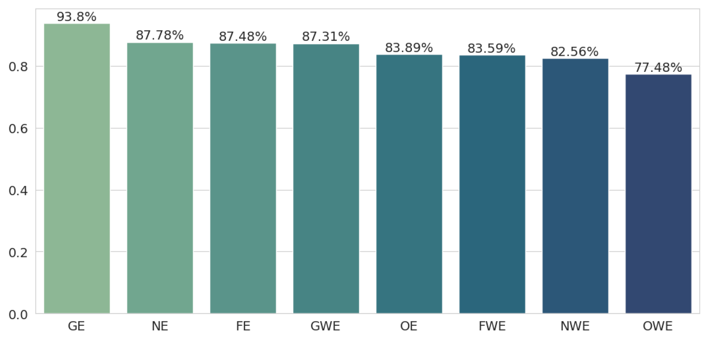
First, text classification was checked by selecting classes for sentences by checking the shortest distance between the mean sentence embedding and the category embedding. Figure 1 shows the accuracy results for all the embedding methods, sorted in descending order for better readability. It turns out that geometric embeddings perform best (93.8%), with a huge lead of 6 percentage points over second place, which was taken by neural embeddings (87.78%).

This is a logical consequence of how these embeddings were trained since the geometrical embeddings underwent the most drastic change and thus were moved the most in space compared to the other methods. Moving them exactly toward the category embeddings at the training level led to better results. The other two methods, namely neural embeddings and fine-tuned embeddings, performed comparably well, both around 87%. Each of the new methods outperformed the original embeddings (83.89%), so all of these methods improved the classification quality.

All the weighted embeddings perform significantly worse than their unweighted counterparts, with a difference of 5 or 6 percentage points, which was expected given that semantic embeddings occur in every sentence in the dataset. It turns out that only the geometrically weighted embeddings outperform the original embeddings.

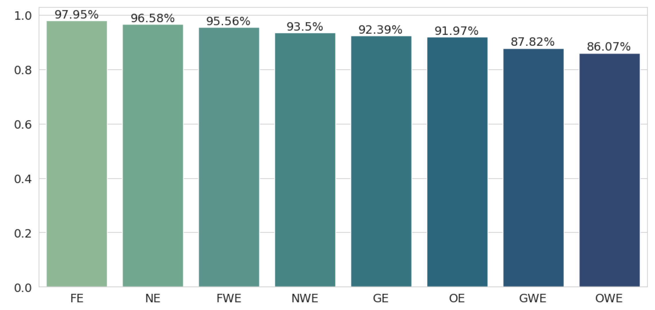
Next, the classification quality was examined using the average sentence embeddings as features for the non-neural text classifiers. The results improved significantly over the previous classification method, and the ranking of the results also changed. This time (see Figure 2), fine-tuned embeddings and neural embeddings were the best, with the latter taking the advantage (97.95% and 96.58%, respectively). The geometric embedding method (92.39%) performed much worse, coming close to the original embeddings’ result (91.97%).

Thus, it seems that despite the stronger shift in the vectors in space in the case of geometric embeddings, they lose some features and the classification suffers. In the case of the mean sentence distance to a category embedding, geometric embeddings showed their full potential, since both the method for creating embeddings and the method for testing them were based on the geometric aspects of vectors in space. In contrast, the Random Forest classification is based on individual features (vector dimensions), and each decision tree in the ensemble model consists of a limited number of features, so it is important that individual features convey as much value as possible, rather than the entire vector as a whole.

Again, weighted embeddings achieve the worse results, although in this case, the difference between weighted embeddings and their unweighted counterparts is much smaller, similar to the difference in the source [40]. However, it turns out that even weighted embeddings, for the neural and fine-tuned methods (95.56% and 93.5%), perform better than the basic version of geometric embeddings (92.39%). Original weighted embeddings perform the worst, with an accuracy drop of almost 12 percentage points (97.95% to 86.07%).

Table 1. Classification results for weighted and unweighted semantic embeddings. (Underline—best results).

Embeddings	Classification with Random Forest	Classification with Mean Sentence Embedding Distance
Original	0.920	0.839
Original Weighted	0.861	0.775
Neural	0.966	0.875
Neural Weighted	0.935	0.836
Fine-tuned	0.979	0.878
Fine-tuned Weighted	0.956	0.826
Geometrical	0.924	0.938
Geometrical Weighted	0.878	0.873

shows a summary of the results for Random Forest classification and mean sentence embedding distance.

4.2. Separability and Spatial Distribution

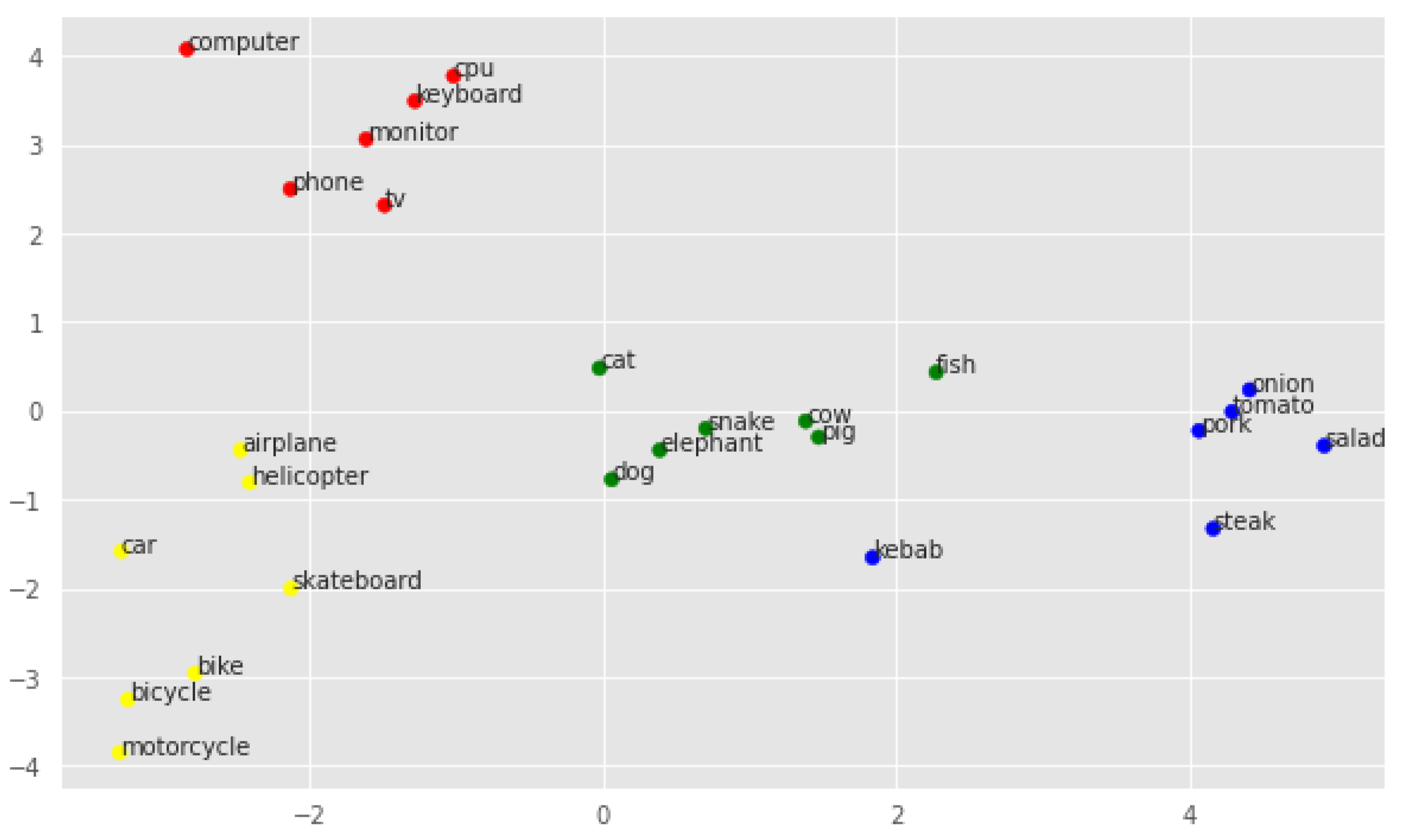
In the next test, the separability of the classes in space and the overall distribution of the vectors were tested. First, the distribution of keyword embeddings in space is shown using the PCA method to reduce dimensionality to two dimensions [43]. Figure 3 shows the distribution of the original embeddings.

As can be seen, even here, the classes seem to be relatively well separated. The classes technology and vehicle seem to be far apart in space, while meal and animal are closer together. Note that the keyword fish is much further away from the other keywords in the cluster, heading towards the category meal. Also, the word kebab seems to be far away from the correct cluster, even though it refers to a meal and does not have a meaning correlated with animals.

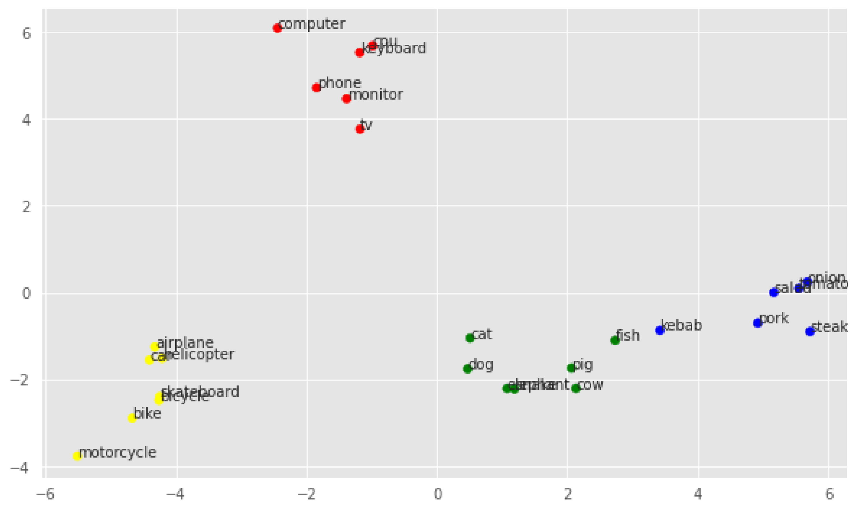
Figure 4 shows a visualization of the PCA for neural embeddings. In this case, the proximity of vectors within classes is visible, and each class becomes more separable. One can see a significant closeness to the corresponding classes of words that were previously more distant, such as fish and kebab, although the latter is somewhere roughly between the centers of the two clusters, so clustering with the K-means algorithm later in this section may still be somewhat problematic.

Figure 5 shows how vectors decompose in two-dimensional space for fine-tuned embeddings, and this method seems to have the worst separability of all the methods so far. Once again, the words fish and kebab, which are separated from their classes while being very close to each other, proved to be problematic. Also, the classes technology and vehicle seem to be more similar to each other, which will be checked with the metrics shown later.

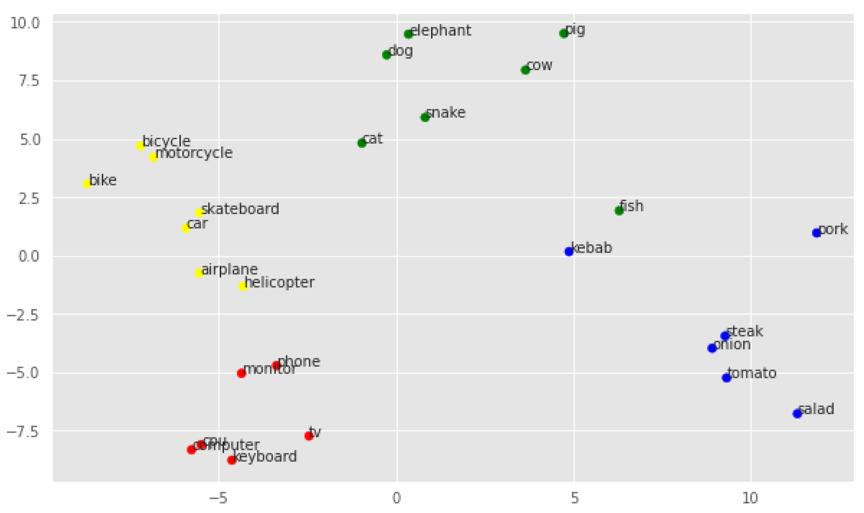
The last of the visualizations of vectors in two-dimensional space using the PCA method concerns geometrical embeddings, as illustrated in Figure 6. In this case, the classes are brilliantly separable, the words within a single cluster are very close to each other, and the problematic cases are resolved. This was to be expected given the nature of the method used to create geometric embeddings, i.e., strong interference with the positions of vectors in space using the $alpha$ and $beta$ parameters.

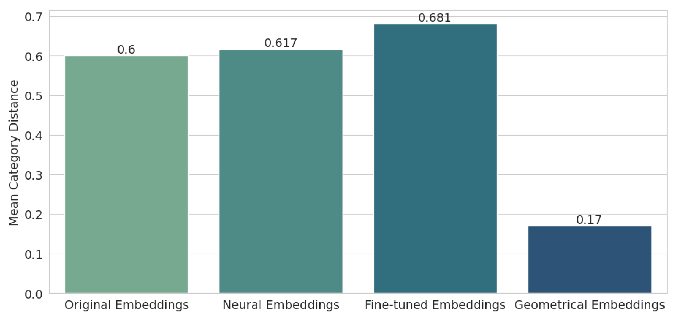
Next, the mean distance from the semantic embeddings to the category embeddings was checked. The results are shown in Figure 7. It turns out that the geometric embeddings are by far the best here (0.17), improving the result of the original embeddings (0.6) by more than three times. The characteristics of the embedding displacement in the space method indicated that it would perform best for this particular test, but the results for the neural embeddings (0.617) and the fine-tuned embeddings (0.681) are surprising, as they were worse compared to the original embeddings.

In order to look deeper into the data, it was decided to also present the mean category distance relative to each category separately. As can be seen in Figure 8, the category that allowed the keyword embeddings to come closest to the category embeddings was the animal category. By far, the worst category in this respect was technology, although the geometric embeddings also did well here (0.201). The only category that managed to improve its performance (excluding geometric embeddings) was the food category, where the neural embeddings (0.614) performed slightly better than the original embeddings (0.631).

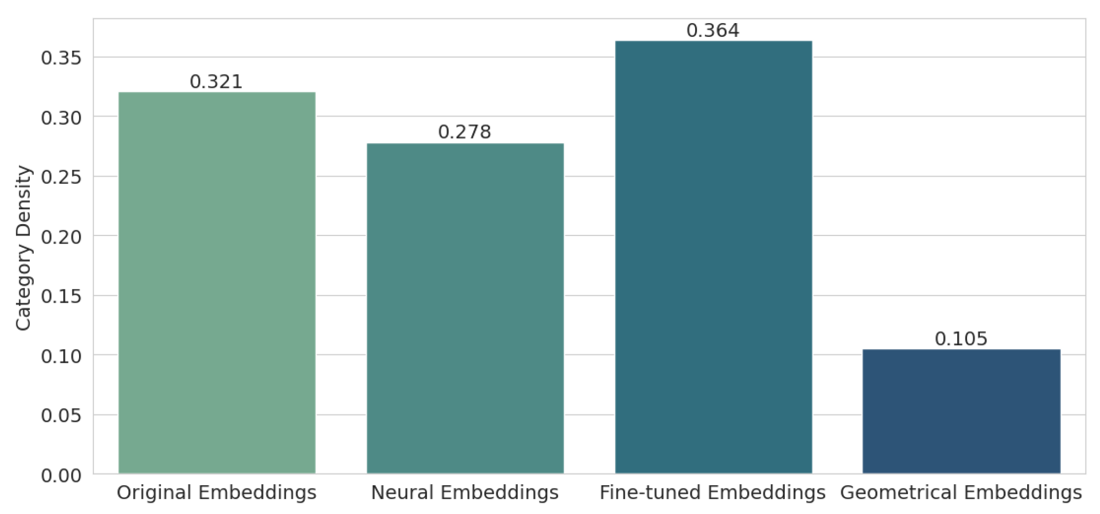
Next, we examined the category density metric, the results of which are shown in Figure 9. Here, the situation looks a bit better, as the results for two methods—neural (0.278) and, of course, geometric (0.105), improved over the original embeddings (0.321). This confirms what was observed when visualizing the PCA for the different types of embeddings, namely that geometric embeddings have excellent separability, and the keywords within classes are very close to each other, while fine-tuned embeddings blur the spatial differences between clusters, and individual words move away from their respective clusters.

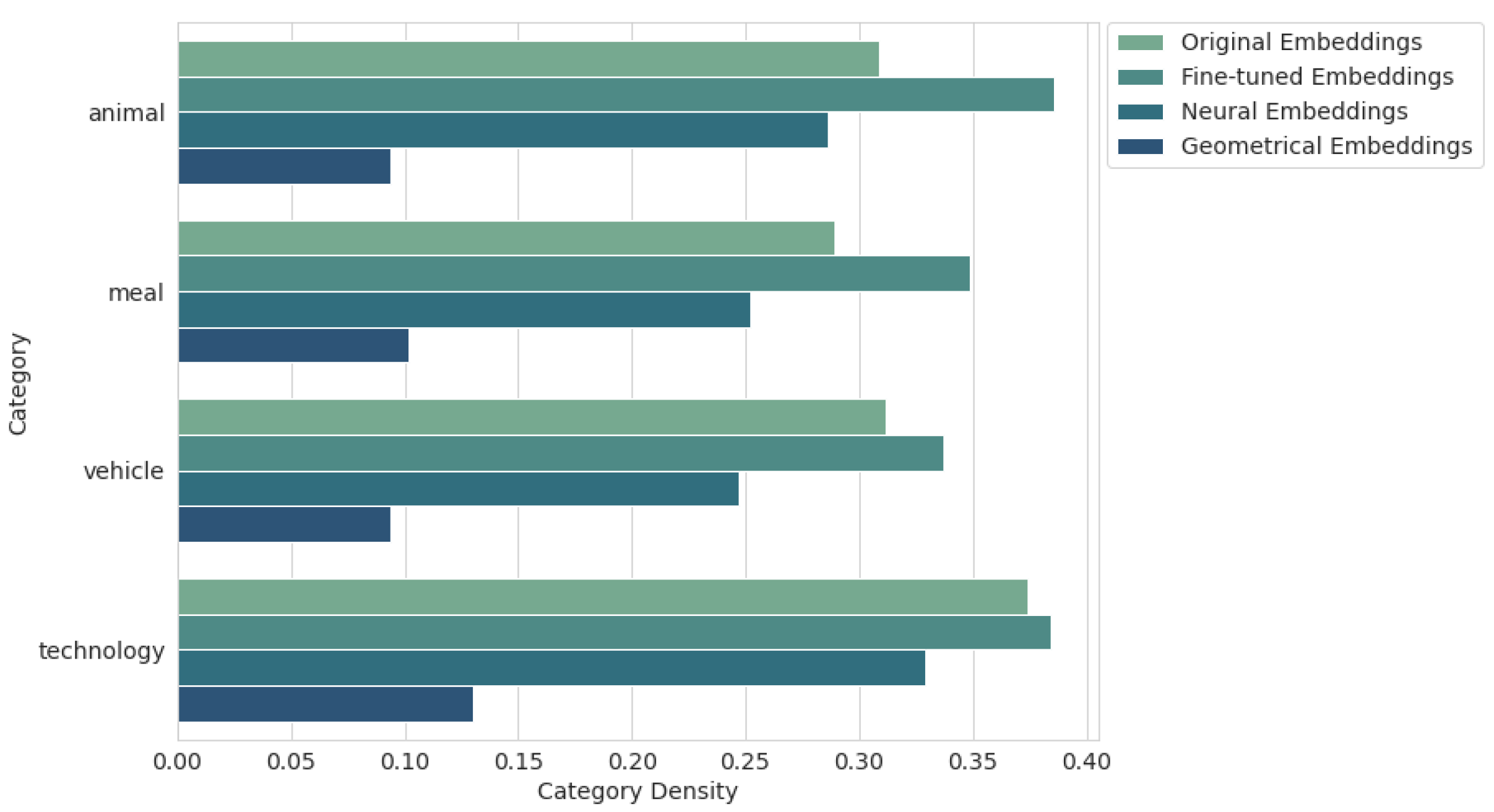
Figure 10 shows the category density results for each category separately. Our suspicion about the problematic meal and animal classes for fine-tuned embeddings, observed in the PCA visualization in Figure 5, was confirmed. In fact, the values for these categories are very high (0.349 and 0.386, respectively), and the technology category also has a low density (0.384). Meanwhile, the least problematic category for most methods is the vehicle class.

The results for the previous two metrics are also reflected in the results for the Silhouette Score. The clusters for the geometric embeddings (0.678) are dense and well separated. The neural embeddings (0.37) still have better cluster quality than the original embeddings (0.24), while the fine-tuned embeddings (0.144) are the worst. Note that none of the embeddings have a silhouette value below zero, so there is little overlap between the categories.

The final test in this section is to see how the K-means method handles class separation.

Table 2. Results for K-means clustering.

Metrics	Original	Neural	Fine-Tuned	Geometrical
Rand Index	1.000	1.000	0.887	1.000
Homogeneity	1.000	1.000	0.747	1.000
Completeness	1.000	1.000	0.762	1.000
V-measure	1.000	1.000	0.754	1.000

shows the results for all metrics tested on the clusters generated by the K-means algorithm, comparing these clusters to the ground truth. It turns out that even in the case of the original embeddings, all these metrics reach the maximum value so that the clustering is performed flawlessly. The same is true for neural and geometric embeddings.

The only method with worse results is again the fine-tuning of pretrained word embeddings, which scores lower than the others for each metric. The misclassified keywords were fish, which was added to the cluster meal instead of animal; phone, which was added to the cluster vehicle instead of technology; and tv, which was added to the cluster animal, instead of technology.

The technology category was the most difficult to cluster correctly. This was not obvious from the PCA visualization (see Figure 5), which only shows the limitations of this method, while it is almost impossible to reduce 300-dimensional data to 2 dimensions without losing relevant information.

Table 3. Summarized results for separability and spatial distribution.

Metrics	Original	Neural	Fine-Tuned	Geometrical
Mean Category Distance	0.600	0.617	0.681	0.170
Category Density	0.321	0.278	0.364	0.105
Silhouette Score	0.240	0.370	0.144	0.678
Rand Index	1.000	1.000	0.887	1.000
Homogeneity	1.000	1.000	0.747	1.000
Completeness	1.000	1.000	0.762	1.000
V-measure	1.000	1.000	0.754	1.000

shows a summary of the results for all metrics. For separability and spatial distribution, the method used to create the geometric embeddings performs by far the best, and the neural embeddings also slightly improve the results compared to the original embeddings. The worst embeddings are the fine-tuned embeddings, which seem to become blurred and degraded during the learning process, which was quite unexpected given that these embeddings performed best for the text classification problem using Random Forest.

5. Discussion

The contribution of our study is the introduction of a supervised method for aligning word embeddings by using the hidden layer of a neural network, their fine-tuning, and vector shifting in the embedding space. For the text classification task, a simpler method that examines the distance between the mean sentence embeddings and category embeddings showed that geometrical embeddings performed best. However, it is important to note that these methods rely heavily on the distance between embeddings, which may not always be the most relevant measure. When using embeddings as input data for the Random Forest classifier, geometrical embeddings performed significantly worse than the other two methods, with fine-tuned embeddings achieving higher accuracy by more than 5 percentage points (97.95% compared to 92.39%).

The implication of this is that when creating embeddings using the vector-shifting method, some information that could be useful for more complex tasks is lost. Additionally, excessively shifting the vectors in space can isolate these embeddings, causing the remaining untrained ones, which intuitively should be close by, to drift apart with each iteration of training. This suggests that for small, isolated sets of semantic word embeddings, geometrical embeddings will perform quite well. However, for open-ended problems with a larger vocabulary and more blurred category boundaries, other methods are likely to be more effective.

While fine-tuned embeddings performed well in the text classification task, they also have their drawbacks. Examining the distribution of vectors in space reveals that embeddings within a class tend to move farther apart, which weakens the semantic relationships between them. This becomes evident in test tasks, such as clustering, where the fine-tuned embeddings performed even worse than the original embeddings. On the other hand, enriching embeddings with domain knowledge improves their performance. Embeddings trained with the GloVe method on specialized texts acquire more semantic depth, as seen in the Random Forest classification results, where they achieved the second-best performance for category queries.

The most well-balanced method appears to be vector training using the trainable embedding layer. Neural embeddings yield very good results for text classification, both with the distance-based method and when using Random Forest. While the embeddings within classes may not be very dense, the classes themselves are highly separable.

6. Conclusions and Future Works

In this paper, we propose a method for aligning word embeddings using a supervised approach that employs the hidden layer of a neural network and shifts the embeddings into the specific categories they correspond to. We evaluate our approach from multiple perspectives: both in an application for supervised and non-supervised tasks and through the analysis of the vector distribution in the representation space. The tests confirm the methods’ usability and provide a deeper understanding of the characteristics of each proposed method.

By comparing our results with state-of-the-art approaches and achieving better accuracy, we confirm the effectiveness of the proposed method. A deep analysis of the vector distributions reveals that there is no one-size-fits-all solution for generating semantic word embeddings; the choice of method should depend on specific design goals and expected outcomes. However, our approach extends traditional methods for creating word vectors.

The results of this research are promising, although some important issues remain unresolved, indicating that further development is needed. The potential applications of semantic word embeddings are vast, and developing new test environments could lead to interesting findings. One rapidly growing area of AI is recommendation systems. McKinsey reports that up to 35% of products purchased on Amazon and 75% of content watched on Netflix come from embedded recommendation systems [45]. Word embedding-based solutions have already been explored and identified as a promising alternative to traditional methods [46].

It is therefore worthwhile to explore whether semantic word embeddings can improve performance. In the context of test environments, embedding weights can be adjusted to enhance prediction accuracy. While IDF weights were used to limit the prediction model, future work could experiment with weights that further emphasize the semantics of the word vectors.

An interesting experiment could involve adding words to the dataset that are strongly associated with multiple categories. For instance, the word jaguar is primarily linked to an animal but also frequently appears in the context of a car brand. It would be valuable to see how different embedding creation methods handle such ambiguous data.

In terms of data modification, leveraging well-established datasets from areas like text classification or information retrieval could be beneficial. This would allow semantic embeddings to be tested on larger datasets and compared against state-of-the-art solutions. The approaches described in this paper have been proven to enhance widely used and well-researched word embedding methods. The $intersect\_word2vec\_format$ method from the Gensim library enables merging the input hidden weight matrix from an existing model with a newly created vocabulary. By setting the lockf parameter to 1.0, the merged vectors can be updated during training.

Another direction worth exploring to extend our research is testing different architectures for embedding creation, particularly with modified cost functions to incorporate semantics. Future research could also expand this to include additional languages, broadening the scope and applicability of these methods.

[custom]