
SCENet: Small Kernel Convolution with Effective Receptive Field Network for Brain Tumor Segmentation


Abstract
1. Introduction
- (1)
- We proposed the Small Kernel Convolution with Effective Receptive Field Network (SCENet) based on UNet, which can effectively improve brain tumor segmentation performance.
- (2)
- We designed an SCER block to enhance the effectiveness and efficiency of extraction of features with effective, receptive filled-in encoder layers.
- (3)
- We used a CSAM attention mechanism to select the more important, detailed features of decoder layers.
- (4)
- The ASPP module was introduced to the bottleneck layer to enlarge the receptive field in order to capture more detailed features.
2. Related Work
2.1. Deep Learning-Based Methods for Medical Image Segmentation
2.2. The Attention-Based Module for Medical Image Segmentation
2.3. Transformer-Based Architecture for Medical Image Segmentation
3. Methodology
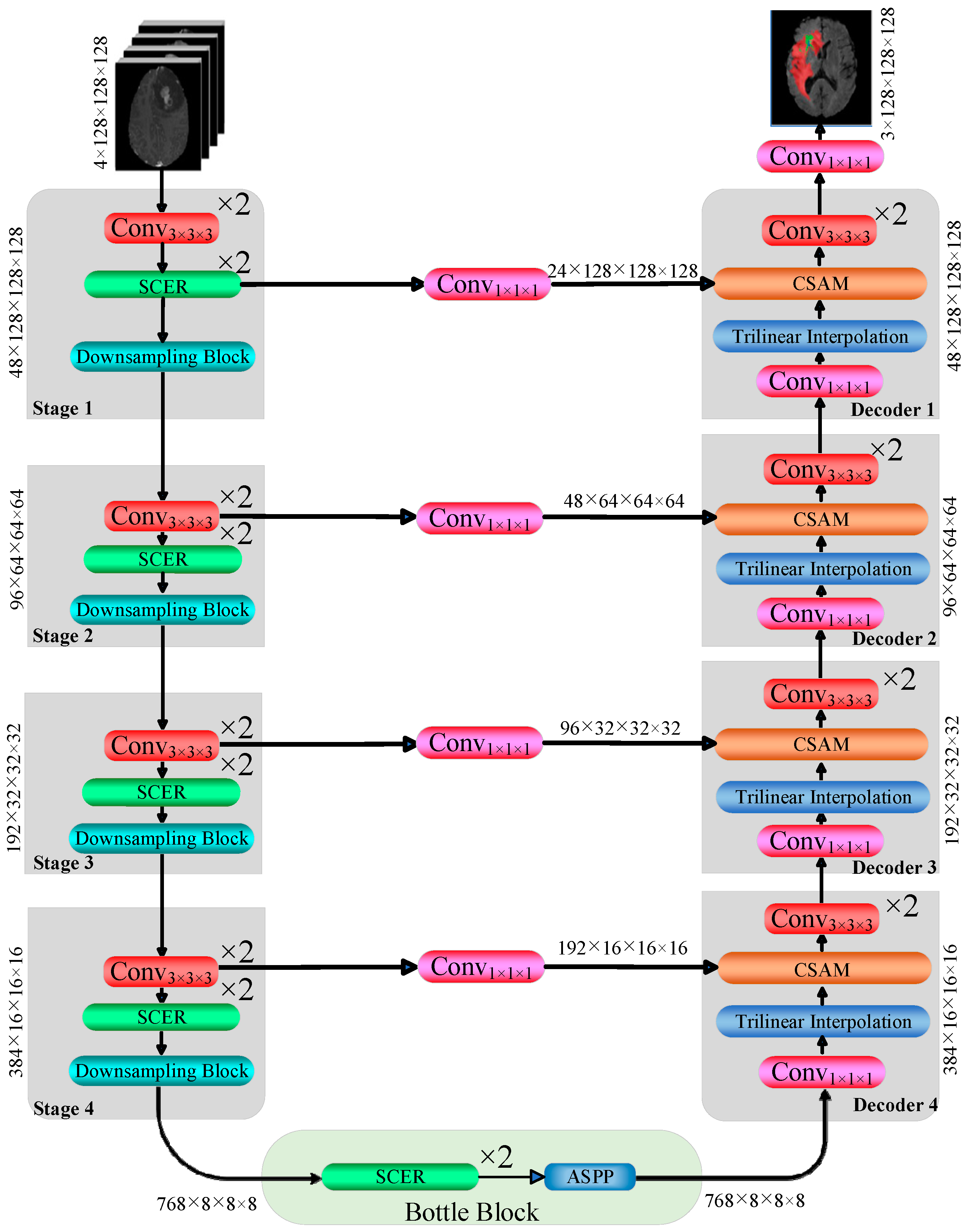
3.1. Network Architecture
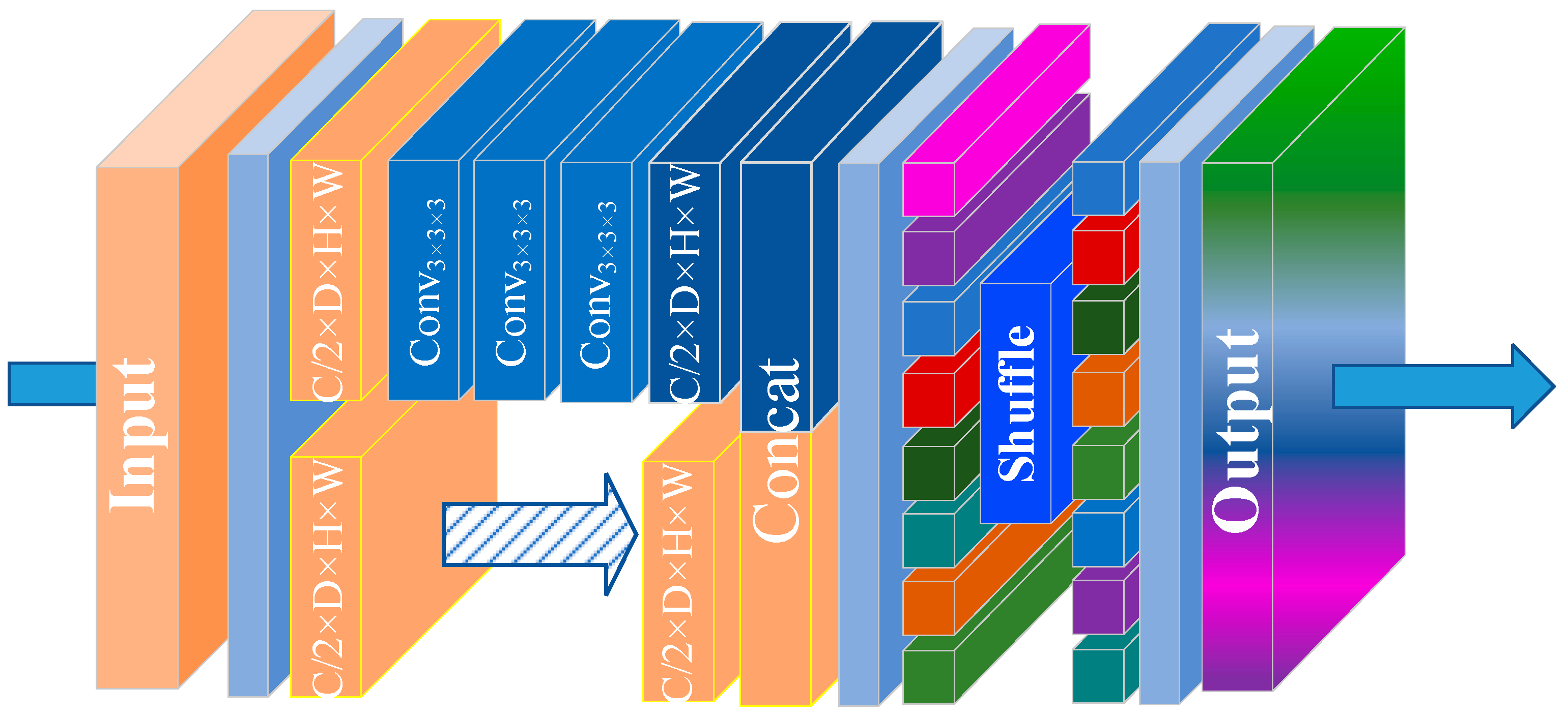
3.2. Small Kernel Convolution with Effective Receptive Field Shuffle Module (SCER)
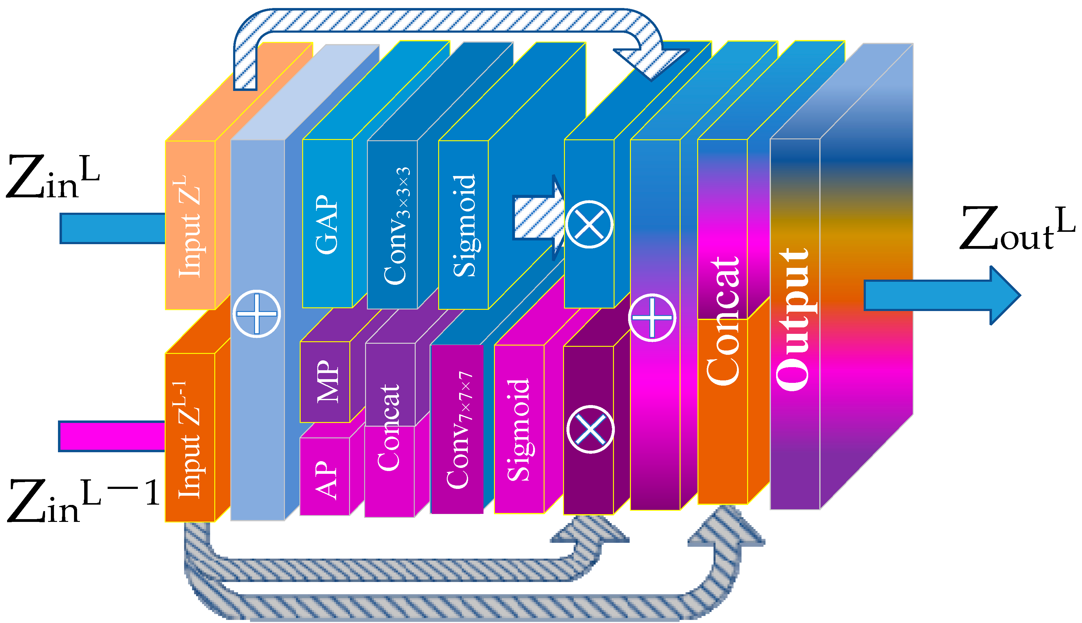
3.3. Channel Spatial Attention Module (CSAM)
4. Experiments and Results
4.1. Datasets and Preprocessing
4.2. Implementation Details
4.3. Evaluation Metrics
4.4. Comparison with Other Methods
4.5. Ablation Experiments
4.5.1. Ablation Study of Each Module in SCENet
4.5.2. Ablation Study of the Number of Stacking Convolution Layers and Kernel Size in the SCER Module
4.5.3. Comparative Experiment SCER Module of SCENet with Shuffle Block of Shufflenet V2
5. Limitations and Future Perspectives
6. Conclusions
Author Contributions
Funding
Institutional Review Board Statement
Informed Consent Statement
Data Availability Statement
Conflicts of Interest
Abbreviations
| AG | Attention Gate |
| AP | Average Pooling |
| ASPP | Atrous Spatial Pyramid Pooling |
| AVG | Average Dice Value |
| CNN | Convolutional Neural Network |
| CSAM | Channel Spatial Attention Module |
| Dice | Dice Similarity Coefficient |
| ET | Enhancing Tumor |
| EVO Norm | Evolving Normalization–Activation Layers |
| Expt | Experiment |
| FCN | Fully Convolutional Networks |
| FLAIR | Fluid Attenuated Inversion Recovery |
| GAP | Global Average Pooling |
| HD | Hausdorff Distance |
| LN | Layer Normalization |
| MP | Max Pooling |
| ROI | Region Of Interest |
| SCENet | Small Kernel Convolution With Effective Receptive Field Network |
| SCER | Small Kernel Convolution With Effective Receptive Field Shuffle Module |
| SGE | Spatial Group-Wise Enhance |
| T1 | T1-Weighted |
| T1ce | T1-Enhanced Contrast |
| T2 | T2-Weighted |
| TC | Tumor Core |
| VIT | Vision Transformer |
| VTUnet | Volumetric Transformer |
| WHO | World Health Organization |
| WT | Whole Tumor |
References
- Ibebuike, K.; Ouma, J.; Gopal, R. Meningiomas among intracranial neoplasms in Johannesburg, South Africa: Prevalence, clinical observations and review of the literature. Afr. Health Sci. 2013, 13, 118–121. [Google Scholar] [CrossRef] [PubMed]
- Herholz, K.; Langen, K.-J.; Schiepers, C.; Mountz, J.M. Brain tumors. Semin. Nucl. Med. 2012, 42, 356–370. [Google Scholar] [CrossRef] [PubMed]
- Wu, J.; Su, R.; Qiu, D.; Cheng, X.; Li, L.; Huang, C.; Mu, Q. Analysis of DWI in the classification of glioma pathology and its therapeutic application in clinical surgery: A case-control study. Transl. Cancer Res. 2022, 11, 805–812. [Google Scholar] [CrossRef]
- Chen, J.; Qi, X.; Zhang, M.; Zhang, J.; Han, T.; Wang, C.; Cai, C. Review on neuroimaging in pediatric-type diffuse low-grade gliomas. Front. Pediatr. 2023, 11, 1149646. [Google Scholar] [CrossRef] [PubMed]
- Verma, N.; Cowperthwaite, M.C.; Burnett, M.G.; Markey, M.K.J. Differentiating tumor recurrence from treatment necrosis: A review of neuro-oncologic imaging strategies. Neuro-Oncology 2013, 15, 515–534. [Google Scholar] [CrossRef]
- Bauer, S.; Wiest, R.; Nolte, L.-P.; Reyes, M. A survey of MRI-based medical image analysis for brain tumor studies. Phys. Med. Biol. 2013, 58, R97. [Google Scholar] [CrossRef]
- Bakas, S.; Akbari, H.; Sotiras, A.; Bilello, M.; Rozycki, M.; Kirby, J.S.; Freymann, J.B.; Farahani, K.; Davatzikos, C. Advancing the cancer genome atlas glioma MRI collections with expert segmentation labels and radiomic features. Sci. Data 2017, 4, 170117. [Google Scholar] [CrossRef]
- Ronneberger, O.; Fischer, P.; Brox, T. U-net: Convolutional networks for biomedical image segmentation. In Proceedings of the Medical Image Computing and Computer-Assisted Intervention–MICCAI 2015: 18th International Conference, Munich, Germany, 5–9 October 2015; pp. 234–241. [Google Scholar]
- Çiçek, Ö.; Abdulkadir, A.; Lienkamp, S.S.; Brox, T.; Ronneberger, O. 3D U-Net: Learning dense volumetric segmentation from sparse annotation. In Proceedings of the Medical Image Computing and Computer-Assisted Intervention–MICCAI 2016: 19th International Conference, Athens, Greece, 17–21 October 2016; pp. 424–432. [Google Scholar]
- LeCun, Y.; Bottou, L.; Bengio, Y.; Haffner, P. Gradient-based learning applied to document recognition. Proc. IEEE 1998, 86, 2278–2324. [Google Scholar] [CrossRef]
- Long, J.; Shelhamer, E.; Darrell, T. Fully convolutional networks for semantic segmentation. In Proceedings of the IEEE Conference on Computer Vision and Pattern Recognition, Boston, MA, USA, 7–12 June 2015; pp. 3431–3440. [Google Scholar]
- Norman, B.; Pedoia, V.; Majumdar, S. Use of 2D U-Net convolutional neural networks for automated cartilage and meniscus segmentation of knee MR imaging data to determine relaxometry and morphometry. Radiology 2018, 288, 177–185. [Google Scholar] [CrossRef]
- Sevastopolsky, A. Optic disc and cup segmentation methods for glaucoma detection with modification of U-Net convolutional neural network. Pattern Recognit. Image Anal. 2017, 27, 618–624. [Google Scholar] [CrossRef]
- Roy, A.G.; Conjeti, S.; Karri, S.P.K.; Sheet, D.; Katouzian, A.; Wachinger, C.; Navab, N. ReLayNet: Retinal layer and fluid segmentation of macular optical coherence tomography using fully convolutional networks. Biomed. Opt. Express. 2017, 8, 3627–3642. [Google Scholar] [CrossRef] [PubMed]
- Skourt, B.A.; El Hassani, A.; Majda, A. Lung CT image segmentation using deep neural networks. Procedia Comput. Sci. 2018, 127, 109–113. [Google Scholar] [CrossRef]
- Chen, C.; Liu, X.; Ding, M.; Zheng, J.; Li, J. 3D dilated multi-fiber network for real-time brain tumor segmentation in MRI. In Proceedings of the Medical Image Computing and Computer Assisted Intervention–MICCAI 2019: 22nd International Conference, Shenzhen, China, 13–17 October 2019; pp. 184–192. [Google Scholar]
- Raza, R.; Bajwa, U.I.; Mehmood, Y.; Anwar, M.W.; Jamal, M.H. dResU-Net: 3D deep residual U-Net based brain tumor segmentation from multimodal MRI. Biomed. Signal Process. Control 2023, 79, 103861. [Google Scholar] [CrossRef]
- Ahmad, P.; Qamar, S.; Shen, L.; Rizvi, S.Q.A.; Ali, A.; Chetty, G. Ms unet: Multi-scale 3d unet for brain tumor segmentation. In Proceedings of the International MICCAI Brainlesion Workshop, Singapore, 18 September 2022; pp. 30–41. [Google Scholar]
- Gammoudi, I.; Ghozi, R.; Mahjoub, M.A. An Innovative Approach to Multimodal Brain Tumor Segmentation: The Residual Convolution Gated Neural Network and 3D UNet Integration. Trait. Signal 2024, 41, 141–151. [Google Scholar] [CrossRef]
- Soni, V.; Singh, N.K.; Singh, R.K.; Tomar, D.S. Multiencoder-based federated intelligent deep learning model for brain tumor segmentation. IMA 2023, 34, e22981. [Google Scholar] [CrossRef]
- Olisah, C.C. SEDNet: Shallow Encoder-Decoder Network for Brain Tumor Segmentation. arXiv 2024, arXiv:2401.13403. [Google Scholar]
- Chen, R.; Lin, Y.; Ren, Y.; Deng, H.; Cui, W.; Liu, W. An efficient brain tumor segmentation model based on group normalization and 3D U-Net. IMA 2024, 34, e23072. [Google Scholar] [CrossRef]
- Oktay, O.; Schlemper, J.; Folgoc, L.L.; Lee, M.; Heinrich, M.; Misawa, K.; Mori, K.; Mcdonagh, S.; Hammerla, N.Y.; Kainz, B.; et al. Attention u-net: Learning where to look for the pancreas. arXiv 2018, arXiv:1804.03999. [Google Scholar]
- Liu, D.; Sheng, N.; He, T.; Wang, W.; Zhang, J.; Zhang, J. SGEResU-Net for brain tumor segmentation. Math. Biosci. Eng. 2022, 19, 5576–5590. [Google Scholar] [CrossRef] [PubMed]
- Tian, W.W.; Li, D.W.; Lv, M.Y.; Huang, P. Axial attention convolutional neural network for brain tumor segmentation with multi-modality mri scans. Brain Sci. 2023, 13, 12. [Google Scholar] [CrossRef]
- Zhang, L.; Lan, C.; Fu, L.; Mao, X.; Zhang, M. Segmentation of brain tumor MRI image based on improved attention module Unet network. SIViP 2023, 17, 2277–2285. [Google Scholar] [CrossRef]
- Liu, D.; Sheng, N.; Han, Y.; Hou, Y.; Liu, B.; Zhang, J. SCAU-net: 3D self-calibrated attention U-Net for brain tumor segmentation. Neural Comput. 2023, 35, 23973–23985. [Google Scholar] [CrossRef]
- Zeeshan Aslam, M.; Raza, B.; Faheem, M.; Raza, A. AML-Net: Attention-based multi-scale lightweight model for brain tumor segmentation in internet of medical things. CAAI Trans. Intell. Technol. 2024; early view. [Google Scholar] [CrossRef]
- Kharaji, M.; Abbasi, H.; Orouskhani, Y.; Shomalzadeh, M.; Kazemi, F.; Orouskhani, M. Brain Tumor Segmentation with Advanced nnU-Net: Pediatrics and Adults Tumors. Neurosci. Inform. 2024, 4, 100156. [Google Scholar] [CrossRef]
- Pang, B.; Chen, L.; Tao, Q.; Wang, E.; Yu, Y. GA-UNet: A Lightweight Ghost and Attention U-Net for Medical Image Segmentation. J. Imaging Inform. Med. 2024, 37, 1874–1888. [Google Scholar] [CrossRef] [PubMed]
- Tang, Y.; Han, K.; Guo, J.; Xu, C.; Xu, C.; Wang, Y. GhostNetV2: Enhance cheap operation with long-range attention. Proc. Adv. Neural Inf. Process. Syst. 2022, 35, 9969–9982. [Google Scholar]
- Peiris, H.; Hayat, M.; Chen, Z.; Egan, G.; Harandi, M. A robust volumetric transformer for accurate 3D tumor segmentation. In Proceedings of the International Conference on Medical Image Computing and Computer-Assisted Intervention, Singapore, 18–22 September 2022; pp. 162–172. [Google Scholar]
- Jia, Q.; Shu, H. Bitr-unet: A cnn-transformer combined network for mri brain tumor segmentation. In Proceedings of the International MICCAI Brainlesion Workshop, Virtual Event, 27 September 2021; pp. 3–14. [Google Scholar]
- Wang, W.; Chen, C.; Ding, M.; Yu, H.; Zha, S.; Li, J. TransBTS: Multimodal brain tumor segmentation using transformer. In Proceedings of the International Conference on Medical Image Computing and Computer-Assisted Intervention, Strasbourg, France, 27 September–1 October 2021; pp. 109–119. [Google Scholar]
- Sun, Q.; Fang, N.; Liu, Z.; Zhao, L.; Wen, Y.; Lin, H. HybridCTrm: Bridging CNN and transformer for multimodal brain image segmentation. J. Healthc. Eng. 2021, 2021, 7467261. [Google Scholar] [CrossRef] [PubMed]
- Hatamizadeh, A.; Tang, Y.; Nath, V.; Yang, D.; Myronenko, A.; Landman, B.; Roth, H.R.; Xu, D. Unetr: Transformers for 3d medical image segmentation. In Proceedings of the IEEE/CVF Winter Conference on Applications of Computer Vision, Waikoloa, HI, USA, 3–8 January 2022; pp. 574–584. [Google Scholar]
- Cai, Y.; Long, Y.; Han, Z.; Liu, M.; Zheng, Y.; Yang, W.; Chen, L. Swin Unet3D: A three-dimensional medical image segmentation network combining vision transformer and convolution. BMC Med. Inform. Decis. Mak. 2023, 23, 33. [Google Scholar] [CrossRef] [PubMed]
- Dosovitskiy, A.; Beyer, L.; Kolesnikov, A.; Weissenborn, D.; Zhai, X.; Unterthiner, T.; Dehghani, M.; Minderer, M.; Heigold, G.; Gelly, S. An image is worth 16 × 16 words: Transformers for image recognition at scale. arXiv 2022, arXiv:2010.11929. [Google Scholar]
- Liu, H.; Brock, A.; Simonyan, K.; Le, Q. Evolving normalization-activation layers. Adv. Neural Inf. Process. Syst. 2020, 33, 13539–13550. [Google Scholar]
- Ba, J.L.; Kiros, J.R.; Hinton, G.E. Layer normalization. arXiv 2016, arXiv:1607.06450. [Google Scholar]
- Chen, L.C.; Papandreou, G.; Kokkinos, I.; Murphy, K.; Yuille, A.L. Deeplab: Semantic image segmentation with deep convolutional nets, atrous convolution, and fully connected CRFs. IEEE Trans. Pattern Anal. Mach. Intell. 2017, 40, 834–848. [Google Scholar] [CrossRef] [PubMed]
- Simonyan, K.; Zisserman, A. Very deep convolutional networks for large-scale image recognition. arXiv 2014, arXiv:1409.1556. [Google Scholar]
- Szegedy, C.; Vanhoucke, V.; Ioffe, S.; Shlens, J.; Wojna, Z. Rethinking the inception architecture for computer vision. In Proceedings of the IEEE Conference on Computer Vision and Pattern Recognition, Las Vegas, NV, USA, 27–30 June 2016; pp. 2818–2826. [Google Scholar]
- Ma, N.; Zhang, X.; Zheng, H.-T.; Sun, J. Shufflenet v2: Practical guidelines for efficient cnn architecture design. In Proceedings of the European Conference on Computer Vision (ECCV), Munich, Germany, 8–14 September 2018; pp. 116–131. [Google Scholar]
- Woo, S.; Park, J.; Lee, J.-Y.; Kweon, I.S. Cbam: Convolutional block attention module. In Proceedings of the European Conference on Computer Vision (ECCV), Munich, Germany, 8–14 September 2018; pp. 3–19. [Google Scholar]
- Baid, U.; Ghodasara, S.; Mohan, S.; Bilello, M.; Calabrese, E.; Colak, E.; Farahani, K.; Kalpathy-Cramer, J.; Kitamura, F.C.; Pati, S. The rsna-asnr-miccai brats 2021 benchmark on brain tumor segmentation and radiogenomic classification. arXiv 2021, arXiv:2107.02314. [Google Scholar]
- Menze, B.H.; Jakab, A.; Bauer, S.; Kalpathy-Cramer, J.; Farahani, K.; Kirby, J.; Burren, Y.; Porz, N.; Slotboom, J.; Wiest, R. The multimodal brain tumor image segmentation benchmark (BRATS). IEEE Trans. Med. Imaging 2014, 34, 1993–2024. [Google Scholar] [CrossRef]
- Lowekamp, B.C.; Chen, D.T.; Ibáñez, L.; Blezek, D. The design of SimpleITK. Front. Neuroinformatics 2013, 7, 45. [Google Scholar] [CrossRef]
- Wright, L.; Demeure, N. Ranger21: A synergistic deep learning optimizer. arXiv 2021, arXiv:2106.13731. [Google Scholar]
- Dice, L.R. Measures of the amount of ecologic association between species. Ecology 1945, 26, 297–302. [Google Scholar] [CrossRef]
- Kim, I.S.; McLean, W. Computing the Hausdorff distance between two sets of parametric curves. Commun. Korean Math. Soc. 2013, 28, 833–850. [Google Scholar] [CrossRef]
- Aydin, O.U.; Taha, A.A.; Hilbert, A.; Khalil, A.A.; Galinovic, I.; Fiebach, J.B.; Frey, D.; Madai, V.I. On the usage of average Hausdorff distance for segmentation performance assessment: Hidden error when used for ranking. Eur. Radiol. Exp. 2021, 5, 4. [Google Scholar] [CrossRef]
- Wu, Q.; Pei, Y.; Cheng, Z.; Hu, X.; Wang, C. SDS-Net: A lightweight 3D convolutional neural network with multi-branch attention for multimodal brain tumor accurate segmentation. Math. Biosci. Eng. 2023, 20, 17384–17406. [Google Scholar] [CrossRef] [PubMed]
- Håversen, A.H.; Bavirisetti, D.P.; Kiss, G.H.; Lindseth, F. QT-UNet: A self-supervised self-querying all-Transformer U-Net for 3D segmentation. IEEE Access 2024, 12, 62664–62676. [Google Scholar] [CrossRef]
- Akbar, A.S.; Fatichah, C.; Suciati, N.; Za’in, C. Yaru3DFPN: A lightweight modified 3D UNet with feature pyramid network and combine thresholding for brain tumor segmentation. Neural Comput. Appl. 2024, 36, 7529–7544. [Google Scholar] [CrossRef]
- Papacocea, S.I.; Vrinceanu, D.; Dumitru, M.; Manole, F.; Serboiu, C.; Papacocea, M.T. Molecular Profile as an Outcome Predictor in Glioblastoma along with MRI Features and Surgical Resection: A Scoping Review. Int. J. Mol. Sci. 2024, 25, 9714. [Google Scholar] [CrossRef] [PubMed]


| Basic Configuration | Value |
|---|---|
 PyTorch Version PyTorch Version | 1.11.0 |
 Python Python | 3.8.10 |
 GPU GPU | NVIDIA RTX A5000 (24G) |
 Cuda Cuda | cu113 |
| Learning Rate | 1 × 10⁴ |
| Optimizer | Ranger |
| Batch Size | 1 |
| Input Size | 128 × 128 × 128 |
| Output Size | 128 × 128 × 128 |
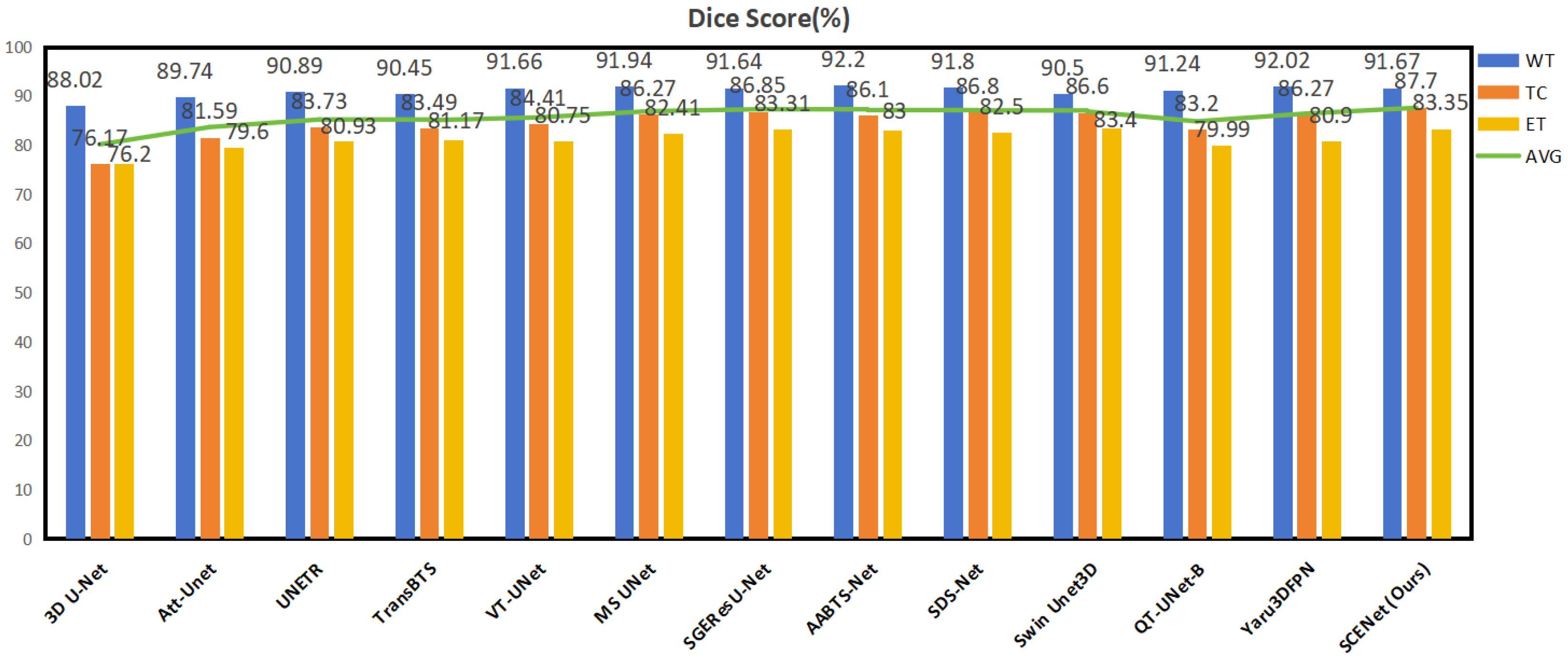
| Methods | Dice (%) | Hausdorff 95 (mm) | Ref. | ||||||
|---|---|---|---|---|---|---|---|---|---|
| WT | TC | ET | AVG | WT | TC | ET | AVG | ||
| 3D U-Net | 88.02 | 76.17 | 76.20 | 80.13 | 9.97 | 21.57 | 25.48 | 19.01 | [9] |
| Att-Unet | 89.74 | 81.59 | 79.60 | 83.64 | 8.09 | 14.68 | 19.37 | 14.05 | [23] |
| UNETR | 90.89 | 83.73 | 80.93 | 85.18 | 4.71 | 13.38 | 21.39 | 13.16 | [36] |
| TransBTS | 90.45 | 83.49 | 81.17 | 85.03 | 6.77 | 10.14 | 18.94 | 11.95 | [34] |
| VT-UNet | 91.66 | 84.41 | 80.75 | 85.61 | 4.11 | 13.20 | 15.08 | 10.80 | [32] |
| MS UNet (2022) | 91.94 | 86.27 | 82.41 | 86.87 | - | - | - | - | [18] |
| SGEResU-Net (2022) | 91.64 | 86.85 | 83.31 | 87.27 | 5.95 | 7.57 | 19.28 | 10.93 | [24] |
| AABTS-Net (2022) | 92.20 | 86.10 | 83.00 | 87.10 | 4.00 | 11.18 | 17.73 | 10.97 | [25] |
| SDS-Net (2023) | 91.80 | 86.80 | 82.50 | 87.03 | 21.07 | 11.99 | 13.13 | 15.40 | [53] |
| Swin Unet3D (2023) | 90.50 | 86.60 | 83.40 | 86.83 | - | - | - | - | [37] |
| QT-UNet-B (2024) | 91.24 | 83.2 | 79.99 | 84.81 | 4.44 | 12.95 | 17.19 | 11.53 | [54] |
| Yaru3DFPN (2024) | 92.02 | 86.27 | 80.9 | 86.4 | 4.09 | 8.43 | 21.91 | 11.48 | [55] |
| SCENet (Ours) | 91.67 | 87.70 | 83.35 | 87.57 | 5.34 | 8.03 | 19.41 | 10.93 | |
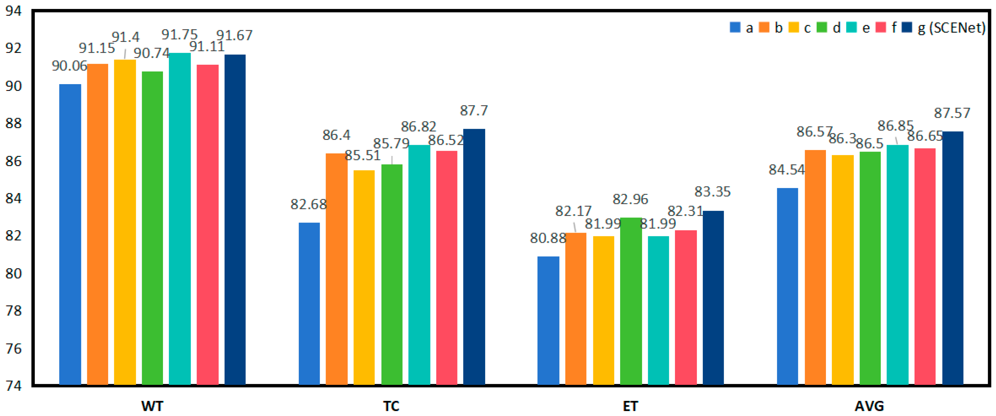
| Expt | SCER | CSAM | ASPP | Dice(%) | |||
| WT | TC | ET | AVG | ||||
| A | 90.06 | 82.68 | 80.88 | 84.54 | |||
| B | √ | 91.15 | 86.40 | 82.17 | 86.57 | ||
| C | √ | 91.40 | 85.51 | 81.99 | 86.30 | ||
| D | √ | 90.74 | 85.79 | 82.96 | 86.50 | ||
| E | √ | √ | 91.75 | 86.82 | 81.99 | 86.85 | |
| F | √ | √ | 91.11 | 86.52 | 82.31 | 86.65 | |
| G (SCENet) | √ | √ | √ | 91.67 | 87.70 | 83.35 | 87.57 |
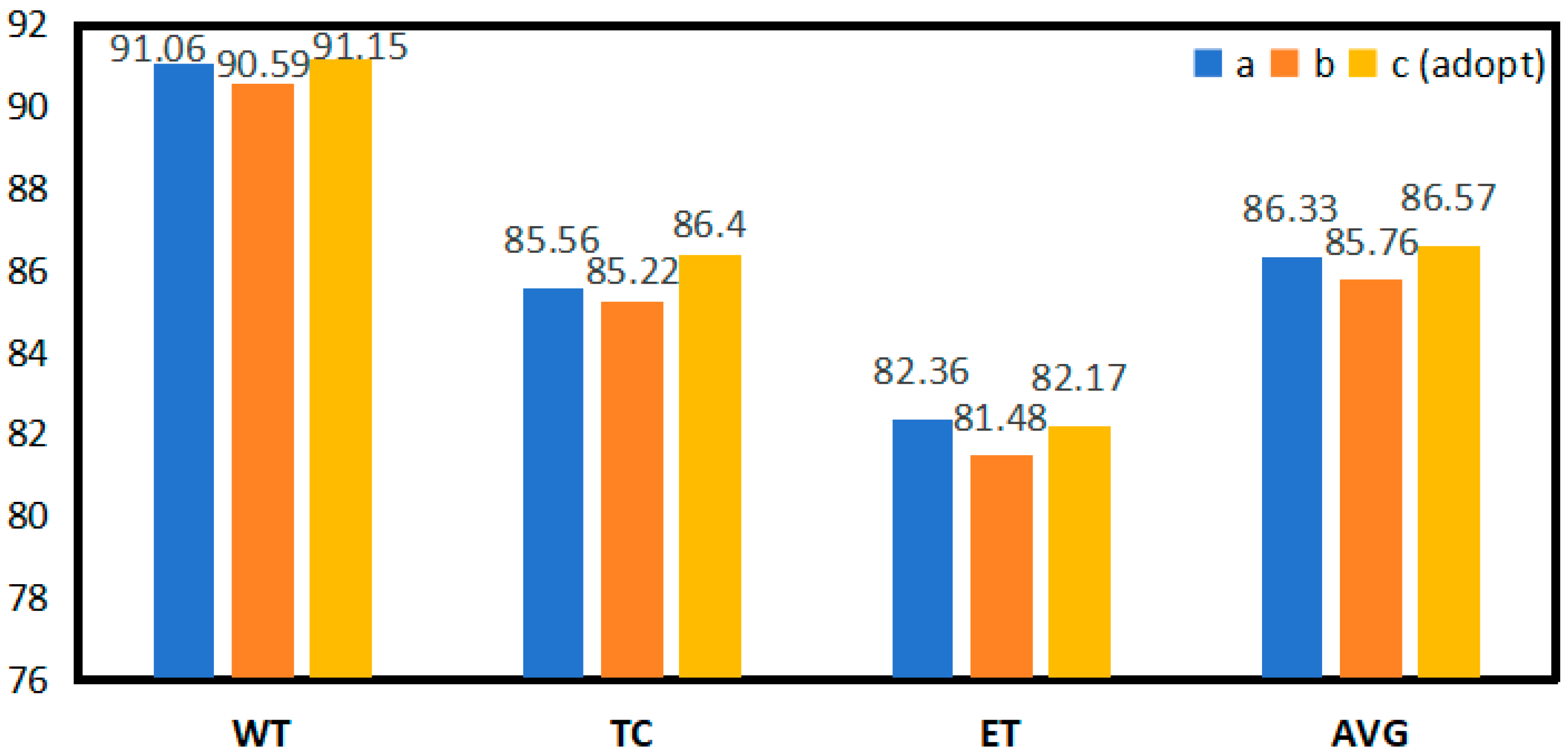
| Expt | Conv Num | Kernel Size | Dice (%) | FLOPs | Parameter | |||
| WT | TC | ET | AVG | |||||
| A | 1 | 7 × 7 × 7 | 91.06 | 85.56 | 82.36 | 86.33 | 2763.476 G | 228.368 M |
| B | 2 | 3 × 3 × 3 | 90.59 | 85.22 | 81.48 | 85.76 | 1410.731 G | 114.840 M |
| C (SCENet) | 3 | 3 × 3 × 3 | 91.15 | 86.40 | 82.17 | 86.57 | 1537.095 G | 125.446 M |
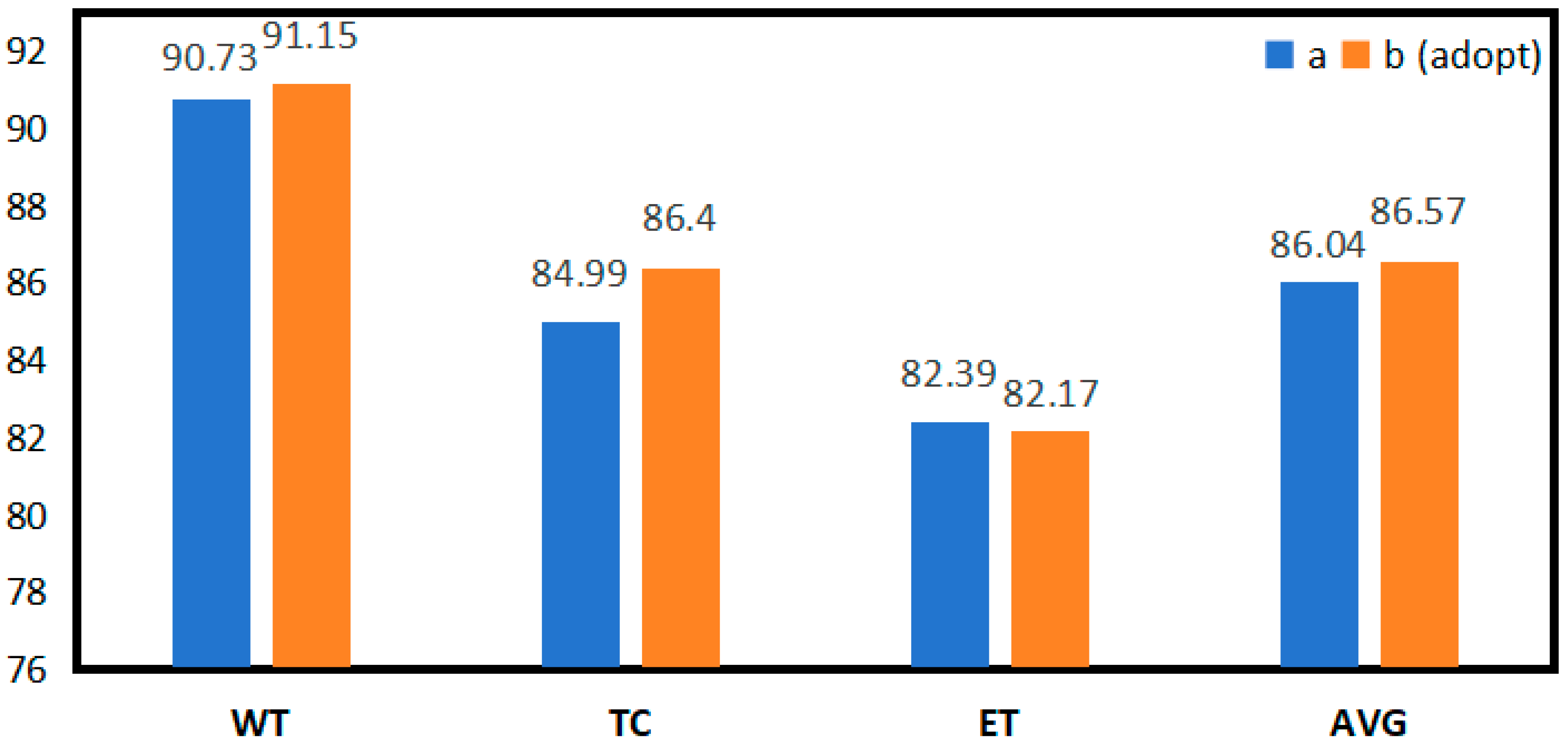
| Expt | Dice(%) | ||||
| WT | TC | ET | AVG | ||
| A | shuffle block | 90.73 | 84.99 | 82.39 | 86.04 |
| B (adopt) | SCER | 91.15 | 86.40 | 82.17 | 86.57 |
Disclaimer/Publisher’s Note: The statements, opinions and data contained in all publications are solely those of the individual author(s) and contributor(s) and not of MDPI and/or the editor(s). MDPI and/or the editor(s) disclaim responsibility for any injury to people or property resulting from any ideas, methods, instructions or products referred to in the content. |
© 2024 by the authors. Licensee MDPI, Basel, Switzerland. This article is an open access article distributed under the terms and conditions of the Creative Commons Attribution (CC BY) license (https://creativecommons.org/licenses/by/4.0/).
Share and Cite
Guo, B.; Cao, N.; Zhang, R.; Yang, P. SCENet: Small Kernel Convolution with Effective Receptive Field Network for Brain Tumor Segmentation. Appl. Sci. 2024, 14, 11365. https://doi.org/10.3390/app142311365
Guo B, Cao N, Zhang R, Yang P. SCENet: Small Kernel Convolution with Effective Receptive Field Network for Brain Tumor Segmentation. Applied Sciences. 2024; 14(23):11365. https://doi.org/10.3390/app142311365
Chicago/Turabian StyleGuo, Bin, Ning Cao, Ruihao Zhang, and Peng Yang. 2024. "SCENet: Small Kernel Convolution with Effective Receptive Field Network for Brain Tumor Segmentation" Applied Sciences 14, no. 23: 11365. https://doi.org/10.3390/app142311365
APA StyleGuo, B., Cao, N., Zhang, R., & Yang, P. (2024). SCENet: Small Kernel Convolution with Effective Receptive Field Network for Brain Tumor Segmentation. Applied Sciences, 14(23), 11365. https://doi.org/10.3390/app142311365