Study of the Characteristics of Second-Order Underdamped Unsaturated Stochastic Resonance System Driven by OFDM Signals

Abstract

Aiming at the issue of suboptimal demodulation performance in OFDM signal enhancement processes due to slow response speeds in first-order overdamped stochastic resonance systems, this paper designs an OFDM signal enhancement and demodulation system based on second-order underdamped unsaturated bistable stochastic resonance (SUUBSR). Firstly, a nonsaturated bistable potential function model is constructed by combining a traditional monostable potential function with a Gaussian potential function, and a damping coefficient is introduced simultaneously to build the SUUBSR system. Subsequently, the transient and steady-state output response analytical expressions of the SUUBSR system under OFDM signal excitation are derived, the energy loss of OFDM symbol waveforms caused by the transient response of the system is discussed, and the relationship between the damping coefficient and the steady-state output response of the system is explored. Finally, simulations are conducted to evaluate the enhancement and demodulation process of OFDM signals using the SUUBSR system. The simulation results show that at an input signal–noise ratio of 2 dB, compared to the first-order unsaturated bistable stochastic resonance (FUBSR) system, the proposed system reduces the system response time by 3.956% of a symbol period and decreases the demodulation bit error rate for OFDM signals by approximately 35%.

1. Introduction

Orthogonal frequency division multiplexing (OFDM) has been widely used in wireless local area networks, mobile communications, and other fields due to its high-frequency band utilization and ease of engineering implementation. In recent years, scholars have been dedicated to research on the detection of weak OFDM signals in complex electromagnetic environments. Stochastic resonance (SR) has broken the traditional concept that noise is harmful in weak signal detection methods, using noise as an energy source to enhance weak signals. Applying the stochastic resonance theory to the detection of OFDM signals has great research significance and application prospects.

Currently, scholars at home and abroad have conducted extensive research on communication signal detection based on stochastic resonance. Ji C et al. [1] applied traditional bistable stochastic resonance to OFDM signal detection, improving the detection effect of OFDM signals. However, due to the limitations of the traditional potential function structure, the system suffers from output saturation issues. Jiao S et al. [2] constructed a new piecewise potential function model to improve the antisaturation performance of the system, but their system model is a first-order system and does not consider the effect of combining a nonsaturating potential function model with a second-order underdamped system. Addressing the poor anti-noise performance of traditional stochastic resonance systems, Zhengmu Ma Z et al. [3] constructed a second-order underdamped periodic potential resonance system, demonstrating that stochastic resonance can occur in second-order underdamped systems. Ding J et al. [4] built a second-order underdamped nonsaturating stochastic resonance system, and the experimental results showed that this system can detect weak signals in different noise environments. Zhang C et al. [5] proposed a signal detection method based on an underdamped tristable stochastic resonance system which exhibits stronger noise suppression capabilities and better signal enhancement effects. Zhai Y et al. [6] theoretically derived the signal–noise ratio formula for second-order underdamped systems, proving that the anti-noise performance of underdamped systems is superior to that of overdamped systems. The aforementioned literature demonstrates the superiority of underdamped systems in signal enhancement but does not analyze and compare the advantages and disadvantages of underdamped and overdamped systems in terms of response speed. Jin Y et al. [7] and Li M et al. [8] derived theoretical formulas for the mean first passage time and particle transition rate of second-order underdamped systems, indirectly proving that underdamped systems respond faster than overdamped systems from the perspective of particle transitions. However, they did not directly discuss system response speed from the perspective of system response. Peng. L et al. [9,10,11,12] proposed a tristable intra-well stochastic resonance system and analyzed its transient stable response, but did not provide a detailed analysis of system response speed and its influencing factors.

Therefore, this paper proposes an enhancement and demodulation system for OFDM signals based on SUUBSR. The main contributions and innovations of this study are as follows:

• A method for enhancing and demodulating OFDM signals based on SUUBSR is proposed.
• OFDM signals are divided into in-phase and quadrature components, which are processed separately by stochastic resonance, addressing the limitation that stochastic resonance systems cannot directly process OFDM signals.
• Analytical expressions for the transient and steady-state responses, as well as time-resolved expressions, of the OFDM signal enhancement and demodulation system based on SUUBSR are theoretically derived. The influence of various parameters on the transient and steady-state responses of the system is analyzed.
• The potential energy loss of OFDM signals during enhancement processing by stochastic resonance is theoretically analyzed.
• The enhancement and demodulation system based on SUUBSR is implemented for OFDM signals with different subcarrier modulation schemes.

Section 2 of this paper introduces the mathematical expressions for the unsaturated potential function model, the OFDM signal model, and the OFDM signal enhancement and demodulation system model based on SUUBSR. Section 3 theoretically derives the analytical expression for the transient and steady-state responses of the system, and analyzes the factors influencing the performance of the proposed system. Section 4 presents the experimental simulations of the proposed method, applying the proposed system to the enhancement and demodulation of communication signals with different carrier modulation schemes to further verify the feasibility and versatility of the proposed system. Section 5 presents all the conclusions of this study, as well as future work and the reasons behind it.

2. Model of Second-Order Underdamped Unsaturated Bistable Stochastic Resonance System Driven by OFDM Signals

This section provides a detailed introduction to the mathematical models of each component of the SUUBSR system driven by OFDM signals, serving as the theoretical foundation for the construction of the SUUBSR system proposed in this paper. Additionally, the overall steps of the OFDM signal enhancement and demodulation algorithm presented in this paper, as well as the method for segmenting OFDM signals, are proposed, providing a theoretical basis for subsequent research work.

2.1. Potential Function Model

The traditional monostable potential function model is the most studied monostable potential function model in stochastic resonance, with the advantages of fewer parameters and the easy adjustment of the potential function structure. Its potential function expression is as follows:

$$U_s(x)={\displaystyle \frac{1}{2}}a{x}^2$$

(1)

where a represents the width of the monostable potential field.

The Gaussian potential function model is a relatively complex monostable potential function model [13]. By adjusting the system parameters, the depth and width of the potential well can be flexibly controlled. Its expression is as follows:

$$U_g(x)=-v\exp (-{\displaystyle \frac{x^2}{r^2}})$$

(2)

where v represents the intensity of the Gaussian potential field, and r represents the depth of the Gaussian potential field.

Combining the advantages of the traditional monostable potential function and Gaussian potential function, this paper introduces the Gaussian potential function on the basis of the traditional monostable potential function and combines the traditional monostable potential function with Gaussian potential function to obtain an unsaturated bistable potential function, which is expressed as follows:

$$U(x)=U_s(x)-U_g(x)={\displaystyle \frac{1}{2}}a{x}^2-(-v\exp (-{\displaystyle \frac{x^2}{r^2}}))$$

(3)

Take the first derivative of the unsaturated bistable potential function, let $U^{\prime }(x)=0$, and when $a{r}^2<2v$, the unsaturated potential function has 2 stable points and 1 unstable point, which are, respectively:

$$\left\{\begin{array}{l}{x}_{s1}=\sqrt{r^2\ln ({\displaystyle \frac{2v}{a{r}^2}})}\\ x_{un}=0\\ x_{s2}=-\sqrt{r^2\ln ({\displaystyle \frac{2v}{a{r}^2}})}\end{array}\right.$$

(4)

2.2. OFDM Baseband Complex Signal Model and the SUUBSR System Model

OFDM Baseband Complex Signal Model

The OFDM baseband signal received by the receiver of the SUUBSR system is as follows:

$$\begin{array}{l}s(t)=\mathrm{Re}\left[{\displaystyle \sum _{m=0}^{M-1}{\displaystyle \sum _{k=0}^{K-1}{d}_{m,k}g}(t-m{T}_s)e^{j\left(2\pi f_{k}t+{\theta }_k\right)}}\right]\\ ={\displaystyle \sum _{m=0}^{M-1}{\displaystyle \sum }_{k=0}^{K-1}\left[{\alpha }_{m,k}\cos (2\pi f_{k}t+{\theta }_k)-{\beta }_{m,k}\sin (2\pi f_{k}t+{\theta }_k)\right]}g\left(t-m{T}_s\right)\end{array}$$

(5)

where M represents the number of subcarriers in the OFDM signal; d_m,k stands for the complex value of the symbol mapped onto the kth subcarrier of the mth OFDM symbol; T_s is the duration of the OFDM signal for one symbol period; and f_k is the frequency of the kth subcarrier.

OFDM signal is a classic multicarrier signal, and each subcarrier is mutually orthogonal. It is relatively difficult to directly perform stochastic resonance processing on OFDM signals using the SUUBSR system. Therefore, the OFDM signal input to the system is first segmented according to the symbol period, and then the signal of one symbol period is decomposed into in-phase and quadrature components through orthogonal transformation, which are sent to two stochastic resonance systems, respectively, for the simultaneous stochastic resonance enhancement processing of these two components. The in-phase and quadrature components within the mth OFDM symbol period can be expressed as follows:

$$\left\{\begin{array}{l}{s}_{\mathrm{I}}(m,n)={\displaystyle \sum _{k=0}^{K-1}{\alpha }_k}\cos \left({\omega }_{k}n+{\theta }_k\right)\\ s_{\mathrm{Q}}(m,n)={\displaystyle \sum _{k=0}^{K-1}{\beta }_k}\sin \left({\omega }_{k}n+{\theta }_k\right)\end{array}\right.$$

(6)

where ${\omega }_k=2\pi f/\Delta f$, $\Delta f$ as the subcarrier spacing, $\Delta f=K/T_s$.

In order to better enhance the OFDM baseband complex signal received by the system through stochastic resonance, this paper constructs the SUUBSR system model, which is divided into I-path and Q-path. The real part and imaginary part of the weak OFDM signal are simultaneously processed by stochastic resonance. The system model is as follows:

$$\left\{\begin{array}{l}{\displaystyle \frac{{\mathrm{d}}^2{x}_{\mathrm{I}}(t)}{\mathrm{d}{t}^2}}=-{\displaystyle \frac{\mathrm{d}U(x_{\mathrm{I}}(t))}{\mathrm{d}{x}_{\mathrm{I}}(t)}}-\gamma {\displaystyle \frac{d{x}_{\mathrm{I}}(t)}{dt}}+s_{\mathrm{I}}(t)+n_{\mathrm{I}}(t)\\ {\displaystyle \frac{{\mathrm{d}}^2{x}_{\mathrm{Q}}(t)}{\mathrm{d}{t}^2}}=-{\displaystyle \frac{\mathrm{d}U(x_{\mathrm{Q}}(t))}{\mathrm{d}{x}_{\mathrm{Q}}(t)}}-\gamma {\displaystyle \frac{d{x}_{\mathrm{Q}}(t)}{dt}}+s_{\mathrm{Q}}(t)+n_{\mathrm{Q}}(t)\end{array}\right.$$

(7)

U(x) is the unsaturated potential function; $\gamma$ is the damping coefficient; the in-phase component of the OFDM baseband complex signal is the input signal for channel I of the system, $s_{\mathrm{I}}(t)$; the quadrature component of the OFDM baseband complex signal is the input signal for channel Q of the system, $s_{\mathrm{Q}}(t)$; the number of subcarriers is N; ${\alpha }_k$ and ${\beta }_k$ represent the real and imaginary parts of the complex value for OFDM symbol mapping, respectively; and $f_k$ and ${\theta }_k$ are, respectively, the frequency and phase of the kth subcarrier. $n_{\mathrm{I}}(t)$ and $n_{\mathrm{Q}}(t)$ represent Gaussian white noise with a mean of 0 and a variance of ${\sigma }^2=2D$, where D denotes the magnitude of the noise intensity. By substituting Equation (3) into Equation (7), the following equation for the SUUBSR is obtained:

$$\left\{\begin{array}{l}{\displaystyle \frac{{\mathrm{d}}^2{x}_{\mathrm{I}}(t)}{\mathrm{d}{t}^2}}={\displaystyle \frac{2v}{r^2}}{x}_{\mathrm{I}}(t)\exp (-{\displaystyle \frac{x_{\mathrm{I}}^2(t)}{r^2}})-a{x}_{\mathrm{I}}(t)-\gamma {\displaystyle \frac{d{x}_{\mathrm{I}}(t)}{dt}}+s_{\mathrm{I}}(t)+n_{\mathrm{I}}(t)\\ {\displaystyle \frac{{\mathrm{d}}^2{x}_{\mathrm{Q}}(t)}{\mathrm{d}{t}^2}}={\displaystyle \frac{2v}{r^2}}{x}_{\mathrm{Q}}(t)\exp (-{\displaystyle \frac{x_{\mathrm{Q}}^2(t)}{r^2}})-a{x}_{\mathrm{Q}}(t)-\gamma {\displaystyle \frac{d{x}_{\mathrm{Q}}(t)}{dt}}+s_{\mathrm{Q}}(t)+n_{\mathrm{Q}}(t)\end{array}\right.$$

(8)

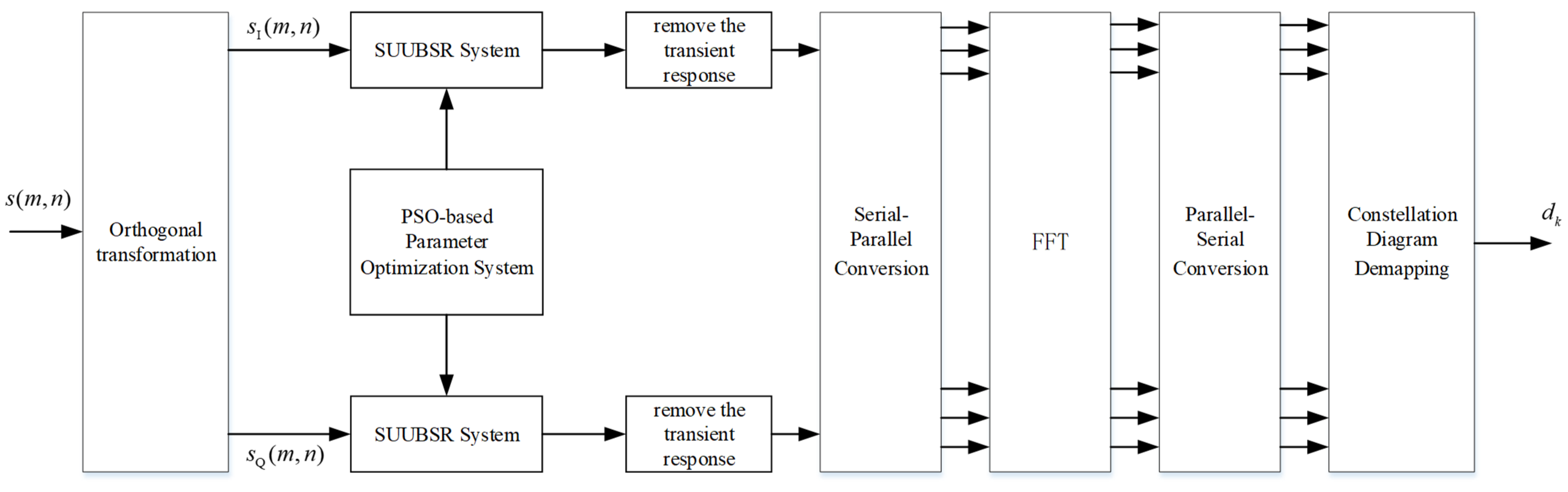
2.3. OFDM Signal Enhancement and Demodulation Model Based on Second-Order Underdamped Unsaturated Stochastic Resonance System

The OFDM signal detection system model based on the SUUBSR system proposed in this paper is shown in Figure 1. In Figure 1, firstly, the received OFDM signal is segmented according to the symbol period, and the orthogonal transform is performed on the OFDM signal waveform within one symbol period to obtain the I-path signal s_I(m,n) and the Q-path signal s_Q(m,n); secondly, the two signals are input into the PSO algorithm parameter optimization system to obtain the optimal parameter sets for the I- and Q-paths of the SUUBSR system, respectively; then, the signals are input into the optimized SUUBSR system, and the transient influence is removed from the two resonance output signals; finally, the signals, after removing the transient response, are demodulated through serial-to-parallel conversion, FFT, parallel-to-serial conversion, constellation inverse mapping, and other steps.

3. Transient Response Analysis of Second-Order Underdamped Stochastic Resonance System Excited by OFDM Signals

Based on the mathematical model of the system proposed in the previous section, in order to theoretically demonstrate the feasibility of the system presented in this paper, this section analyzes the performance of the proposed system from three aspects: first passage time of system response, transient response, and steady-state response. Furthermore, a theoretical comparative analysis is conducted on the response of the SUUBSR system and the FUBSR system.

3.1. First Passage Time Analysis of System Response

The mean first passage time (MFPT) [14,15,16] is one of the indicators reflecting the response speed of the system, which is defined as the average time for a Brownian particle to make the first transition from an initial steady-state point to another steady-state point. Since the methods for solving the MFPT of the I- and Q-channels of the system are the same, the following analysis takes the Q-channel of the system as an example, and the MFPT of the I-channel can be obtained in the same way. Firstly, let $d{x}_{\mathrm{Q}}(t)/dt=y_{\mathrm{Q}}(t)$, and reduce the Q-channel system’s analytical expression in Equation (6) to a one-dimensional system of equations:

$$\left\{\begin{array}{l}{\displaystyle \frac{d{x}_{\mathrm{Q}}(t)}{dt}}=y_{\mathrm{Q}}(t)\\ {\displaystyle \frac{d{y}_{\mathrm{Q}}(t)}{dt}}={\displaystyle \frac{2v}{r^2}}{x}_{\mathrm{Q}}(t)\exp (-{\displaystyle \frac{x_{\mathrm{Q}}^2(t)}{r^2}})-a{x}_{\mathrm{Q}}(t)-\gamma y_{\mathrm{Q}}(t)+s_{\mathrm{Q}}(t)+n_{\mathrm{Q}}(t)\end{array}\right.$$

(9)

Secondly, the steady-state probability density function $\rho (x_{\mathrm{Q}},y_{\mathrm{Q}},t)$ of the system in state $\left(x_{\mathrm{Q}},y_{\mathrm{Q}}\right)$ at time t is derived through the Fokker–Planck equation, which is expressed as follows:

$${\displaystyle \frac{\partial \rho (x_{\mathrm{Q}},y_{\mathrm{Q}},t)}{\partial t}}=D{\displaystyle \frac{{\partial }^2}{\partial {y_{\mathrm{Q}}}^2}}\rho (x_{\mathrm{Q}},y_{\mathrm{Q}},t)-{\displaystyle \frac{\partial }{\partial x_{\mathrm{Q}}}}[y_{\mathrm{Q}}\rho (x_{\mathrm{Q}},y_{\mathrm{Q}},t)]-{\displaystyle \frac{\partial }{\partial y_Q}}\{[f(x_{\mathrm{Q}})-\gamma y_{\mathrm{Q}}]\rho (x_{\mathrm{Q}},y_{\mathrm{Q}},t)\}$$

(10)

Let $\partial \rho (x_{\mathrm{Q}},y_{\mathrm{Q}},t)/\partial t=0$; according to the detailed balance condition [17,18,19], derive the conditions satisfied by the stationary probability density function ${\rho }_s(x_{\mathrm{Q}},y_{\mathrm{Q}},t)$:

$$\left\{\begin{array}{l}{\displaystyle \frac{\partial }{\partial x_{\mathrm{Q}}}}[y_{\mathrm{Q}}{\rho }_s(x_{\mathrm{Q}},y_{\mathrm{Q}},t)]-{\displaystyle \frac{\partial }{\partial y_Q}}\{[U(x_{\mathrm{Q}}){]}^{\prime }{\rho }_s(x_{\mathrm{Q}},y_{\mathrm{Q}},t)\}=0\\ \gamma y_{\mathrm{Q}}{\rho }_s(x_{\mathrm{Q}},y_{\mathrm{Q}},t)+D{\displaystyle \frac{\partial {\rho }_s(x_{\mathrm{Q}},y_{\mathrm{Q}},t)}{\partial y_{\mathrm{Q}}}}=0\end{array}\right.$$

(11)

The steady-state probability density function expression can be derived from Equation (11):

$${\rho }_s(x_{\mathrm{Q}},y_{\mathrm{Q}},t)=P\exp \left(-{\displaystyle \frac{\tilde{U}(x_{\mathrm{Q}},y_{\mathrm{Q}},t)}{D}}\right)$$

(12)

where P is the normalization constant, and $\tilde{U}(x_{\mathrm{Q}},y_{\mathrm{Q}},t)$ is the generalized potential function, which is expressed as follows:

$$\tilde{U}(x_{\mathrm{Q}},y_{\mathrm{Q}},t)=\gamma ({\displaystyle \frac{1}{2}}{y}_{\mathrm{Q}}^2+U(x_{\mathrm{Q}})-x_{\mathrm{Q}}{\displaystyle \sum _{k=0}^{K-1}{\beta }_k}\sin \left(2\pi f_{k}t+{\theta }_k\right))$$

(13)

Then, in Equation (9), let ${\displaystyle \frac{d{y}_{\mathrm{Q}}(t)}{dt}}=0$, ${\displaystyle \frac{d{x}_{\mathrm{Q}}(t)}{dt}}=0$, $D=0$, and ${\beta }_k=0$, then the values of the three singular points are determined, $Q_{u1}(x_{s1},0)$, $Q_{u2}(x_{s2},0)$, and $Q_{un}(x_{un},0)$. And, the expression of the Hessian matrix of Equation:

$$H=\left[\begin{array}{l}0\\ M_x\end{array}\right.\left.\begin{array}{l}1\\ -\gamma \end{array}\right]$$

(14)

In the matrix $H$, the expression for M_x is as follows:

$$M_x=-4x_{\mathrm{Q}}^2\exp (-x_{\mathrm{Q}}^2)+2\exp (-x_{\mathrm{Q}}^2)-a$$

(15)

And then, the corresponding eigenvalues of matrix H at the three singular points $Q_{u1}$, $Q_{u2}$, and $Q_{un}$ in Formula (14) are obtained as ${\lambda }_{s1}^{\pm }$, ${\lambda }_{s2}^{\pm }$, and ${\lambda }_{un}^{\pm }$, respectively.

$$\begin{array}{l}{\lambda }_{s1}^{\pm }={\displaystyle \frac{-\gamma \pm \sqrt{{\gamma }^2-4U^{″}\left(x_{s1}\right)}}{2}}\\ {\lambda }_{s2}^{\pm }={\displaystyle \frac{-\gamma \pm \sqrt{{\gamma }^2-4U^{″}\left(x_{s2}\right)}}{2}}\\ {\lambda }_{un}^{\pm }={\displaystyle \frac{-\gamma \pm \sqrt{{\gamma }^2-4U^{″}\left(x_{un}\right)}}{2}}\end{array}$$

(16)

According to the bistable theory and the two-state model theory, the transition rate of particles between the two stable states can be expressed as follows:

$$R_{1,2}(t)={\displaystyle \frac{1}{2\pi }}\sqrt{{\displaystyle \frac{{\lambda }_{s1}^{+}{\lambda }_{s1}^{-}{\lambda }_{un}^{+}}{\left|{\lambda }_{un}^{-}\right|}}}\exp \left({\displaystyle \frac{\tilde{U}\left(x_{s1},0,t\right)-\tilde{U}\left(x_{un},0,t\right)}{D}}\right)$$

(17)

$$R_{2,1}(t)={\displaystyle \frac{1}{2\pi }}\sqrt{{\displaystyle \frac{{\lambda }_{s2}^{+}{\lambda }_{s2}^{-}{\lambda }_{un}^{+}}{\left|{\lambda }_{un}^{-}\right|}}}\exp \left({\displaystyle \frac{\tilde{U}\left(x_{s2},0,t\right)-\tilde{U}\left(x_{un},0,t\right)}{D}}\right)$$

(18)

Finally, the expression for the average time of the system’s first transition from the steady-state point $x_{s1}$ to the steady-state point $x_{s2}$, also known as the MFPT of the system, is derived from Equations (16)–(18).

$$T_{12}=T(x_{s1}\to x_{s2})=2\pi \sqrt{{\displaystyle \frac{\left|{\lambda }_{un}^{-}\right|}{{\lambda }_{s1}^{+}{\lambda }_{s1}^{-}{\lambda }_{un}^{+}}}}\exp \left({\displaystyle \frac{\tilde{U}\left(x_{un},0,0\right)-\tilde{U}\left(x_{s2},0,0\right)}{D}}\right)$$

(19)

As can be seen from the graph in Figure 2 showing the relationship between the damping coefficient and the MFPT of the particle, when the noise intensity remains constant, as the damping coefficient increases, the MFPT of the particle also increases, indicating that the presence of the damping coefficient causes the particle to be disturbed by damping forces during the transition, hindering the particle’s movement. Conversely, when the damping coefficient remains constant, the greater the noise intensity, the shorter the mean first passage time of the particle, suggesting that during the particle’s motion, the noise energy is converted into kinetic energy required for the particle’s transition, promoting the particle’s transition.

3.2. Transient Steady-State Response Analysis of Underdamped Stochastic Resonance System

3.2.1. Transient Response Theory Derivation

At the beginning of the second-order underdamped nonsaturated bistable stochastic resonance process, the particle does not immediately undergo transition, but randomly selects one of the two potential wells as the initial potential well for particle motion, and performs a local periodic oscillation motion, namely the intra-well motion, for a certain period of time within the initial potential well. This process is the transient response process of the system, and the corresponding time is the transient response time. In order to better study the transient response of the system, the Q-channel of the system is also selected for analysis. The output of the Q-channel of the system is $x_{\mathrm{Q}}(t)$, and the system output is only related to the motion of the particle within the initial well. Then, the nonsaturated bistable potential function can be equivalently regarded as two monostable potential functions, whose expressions are as follows, respectively:

$$U_{+}^{*}(x_{\mathrm{Q}})\approx U^{\prime }(x_{s1}){(x_{\mathrm{Q}}-x_{s1})}^2/2$$

(20)

$$U_{-}^{*}(x_{\mathrm{Q}})\approx U^{\prime }(x_{s2}){(x_{\mathrm{Q}}-x_{s2})}^2/2$$

(21)

where the steady-state points $x_{s1}$ and $x_{s2}$ satisfy the following:

$$\left\{\begin{array}{l}{U}^{\prime }(x_{\mathrm{Q}})={\displaystyle \frac{2v}{r^2}}{x}_{\mathrm{Q}}\exp (-{\displaystyle \frac{{x_{\mathrm{Q}}}^2}{r^2}})-a{x}_{\mathrm{Q}}-s_{\mathrm{Q}}(t)=0\hfill \\ U^{\prime \prime }(x_{\mathrm{Q}})>0\hfill \end{array}\right.$$

(22)

Consequently, the motion equations of the particle near the two stable points of the unsaturated potential function under the influence of a second-order underdamped system are obtained as follows:

$${\displaystyle \frac{{\mathrm{d}}^2{x}_{\mathrm{Q}+}(t)}{\mathrm{d}{t}^2}}=-U^{″}(x_{s1})(x_{\mathrm{Q}+}(t)-x_{s1})-\gamma {\displaystyle \frac{d{x}_{\mathrm{Q}+}(t)}{dt}}+n_{\mathrm{Q}+}(t)$$

(23)

$${\displaystyle \frac{{\mathrm{d}}^2{x}_{\mathrm{Q}-}(t)}{\mathrm{d}{t}^2}}=-U^{″}(x_{s2})(x_{\mathrm{Q}-}(t)-x_{s2})-\gamma {\displaystyle \frac{d{x}_{\mathrm{Q}-}(t)}{dt}}+n_{\mathrm{Q}-}(t)$$

(24)

Based on Equations (23) and (24), the motion of the particle within the left and right wells can be represented by the following deterministic equations:

$${\displaystyle \frac{{\mathrm{d}}^2{x}_{\mathrm{Q}+}(t)}{\mathrm{d}{t}^2}}=-b{x}_{\mathrm{Q}+}(t)-\gamma {\displaystyle \frac{d{x}_{\mathrm{Q}+}(t)}{dt}}+n_{\mathrm{Q}+}(t)$$

(25)

$${\displaystyle \frac{{\mathrm{d}}^2{x}_{\mathrm{Q}-}(t)}{\mathrm{d}{t}^2}}=-b{x}_{\mathrm{Q}-}(t)-\gamma {\displaystyle \frac{d{x}_{\mathrm{Q}-}(t)}{dt}}+n_{\mathrm{Q}-}(t)$$

(26)

When a weak baseband OFDM signal $s(t)$ is input into the system, the input signal is segmented according to the symbol period and subjected to orthogonal transformation to obtain the OFDM complex baseband signal of each symbol period. At this time, the system has Q input signals denoted as $s_{\mathrm{Q}}(t)$, and the output $x_{\mathrm{Q}\pm }(t)$ within the left and right potential wells can be expressed by the following equation:

$$x_{\mathrm{Q}+}(t)={\langle x_{\mathrm{Q}}(t)\rangle }_0+{\displaystyle {\int }_{-\infty }^{T_d}\left[{\displaystyle \sum _{k=0}^{K-1}{\beta }_k}\sin \left(2\pi f_k\tau +{\theta }_k\right)\right]}.h(t-\tau )d\tau$$

(27)

$$x_{\mathrm{Q}-}(t)={\langle x_{\mathrm{Q}}(t)\rangle }_0+{\displaystyle {\int }_{-\infty }^{T_d}\left[{\displaystyle \sum _{k=0}^{K-1}{\beta }_k}\sin \left(2\pi f_k\tau +{\theta }_k\right)\right]}.h(t-\tau )d\tau$$

(28)

$$s_{\mathrm{Q}}(t)={\displaystyle \sum _{k=0}^{K-1}{\beta }_k}\sin \left(2\pi f_k\tau +{\theta }_k\right)$$

(29)

where ${〈x_{\mathrm{Q}}(t)〉}_0$ represents the average response value of the system output when there is no signal input, and $T_d$ is the transient response time. $h(t)$ is the SUUBSR system response function, and its equation is expressed as follows:

$$h(t)=-{\displaystyle \frac{u(t)}{D}}{\displaystyle \frac{\mathrm{d}}{\mathrm{d}t}}{K}_{xx}^0(t)$$

(30)

In the equation, $u(t)=\left\{\begin{array}{l}0,t<0\hfill \\ 1,t>0\hfill \end{array}\right.$ represents the unit step function, and $K_{xx}^0(\tau ,D)$ is the autocorrelation function of the SUUBSR system without being disturbed by an external periodic signal, which is described as follows:

$$K_{xx}^0(\tau ,D)=x_{s1,2}^2\exp \left(-2R_{1,2}\tau \right)$$

(31)

Without the addition of external noise, under the combined influence of a SUUBSR system and a weak OFDM signal, the equation of motion for the particle within the initial trap is as follows:

$${\displaystyle \frac{{\mathrm{d}}^2{x}_{\mathrm{Q}}(t)}{\mathrm{d}{t}^2}}=-b{x}_{\mathrm{Q}}(t)-\gamma {\displaystyle \frac{d{x}_{\mathrm{Q}}(t)}{dt}}+{\displaystyle \sum _{k=0}^{K-1}{\beta }_k}\sin \left(2\pi f_{k}t+{\theta }_k\right)$$

(32)

The general solution to Equation (32) is as follows:

$$x_{\mathrm{Q}}(t)=e^{-{\displaystyle \frac{\gamma }{2}}t}\left[C_1\sin \left({\displaystyle \frac{\sqrt{4b-{\gamma }^2}}{2}}t\right)+\left[C_2\cos \left({\displaystyle \frac{\sqrt{4b-{\gamma }^2}}{2}}t\right)\right]\right]-{\displaystyle \frac{{\mathrm{e}}^{-2R_{1,2}t}{r}^2}{D}}\cdot \ln \left({\displaystyle \frac{2v}{k{r}^2}}\right).{\displaystyle \int {\displaystyle \sum _{k=0}^{K-1}{\beta }_k}}\sin \left(2\pi f_{k}t+{\theta }_k\right){\mathrm{e}}^{2R_{1,2}t}dt$$

(33)

Substitute the initial conditions $t=0$, $x_{\mathrm{Q}}(0)=0$, and $x_{\mathrm{Q}}^{\prime }(0)=0$ into Formula (33) to obtain the values of the undetermined coefficients C₁ and C₂ in the general solution.

$$C_1=\ln \left({\displaystyle \frac{2v}{a{r}^2}}\right){\displaystyle \sum _{k=0}^{K-1}\frac{2\pi f_k{\beta }_k\gamma (\sin {\theta }_k+R_{1,2}\cos {\theta }_k)}{4D{R_{1,2}}^2(1+\frac{{\pi }^2{f_k}^2}{{R_{1,2}}^2})\sqrt{(4b-{\gamma }^2)}}}$$

(34)

$$C_2=-\ln \left({\displaystyle \frac{2v}{a{r}^2}}\right){\displaystyle \sum _{k=0}^{K-1}\frac{r^2{\beta }_k\left(R_{1,2}\sin {\theta }_k-\cos {\theta }_k\right)}{2D{R_{1,2}}^2(1+\frac{{\pi }^2{f_k}^2}{{R_{1,2}}^2})}}$$

(35)

By substituting C₁ and C₂ into Equation (33), the expression for the transient response of the particle’s motion within one symbol period in the SUUBSR system is determined.

$$\begin{array}{l}{x}_{\mathrm{Q}}(t)=\ln \left({\displaystyle \frac{2v}{a{r}^2}}\right)e^{-{\displaystyle \frac{\gamma }{2}}t}{\displaystyle \sum _{k=0}^{K-1}\frac{2\pi f_k{A}_k\gamma (\sin {\theta }_k+R_{1,2}\cos {\theta }_k)}{4D{R_{1,2}}^2(1+\frac{{\pi }^2{f_k}^2}{{R_{1,2}}^2})\sqrt{(4b-{\gamma }^2)}}}\sin \left({\displaystyle \frac{\sqrt{4b-{\gamma }^2}}{2}}t\right)\\ +\ln \left({\displaystyle \frac{2v}{a{r}^2}}\right)e^{-{\displaystyle \frac{\gamma }{2}}t}{\displaystyle \sum _{k=0}^{K-1}\frac{r^2{\beta }_k\left(R_{1,2}\sin {\theta }_k-\cos {\theta }_k\right)}{2D{R_{1,2}}^2(1+\frac{{\pi }^2{f_k}^2}{{R_{1,2}}^2})}}\cos \left({\displaystyle \frac{\sqrt{4b-{\gamma }^2}}{2}}t\right)\\ +\ln \left({\displaystyle \frac{2v}{a{r}^2}}\right){\displaystyle \sum _{k=0}^{K-1}\frac{r^2{\beta }_k\cos (2\pi f_{k}t+{\theta }_k)}{2D{R_{1,2}}^2(1+\frac{{\pi }^2{f_k}^2}{{R_{1,2}}^2})}}-\ln \left({\displaystyle \frac{2v}{a{r}^2}}\right){\displaystyle \sum _{k=0}^{K-1}\frac{r^2{A}_k\sin (2\pi f_{k}t+{\theta }_k)}{2D{R}_{1,2}(1+\frac{{\pi }^2{f_k}^2}{{R_{1,2}}^2})}}\end{array}$$

(36)

where $0<t<T_d$. Similarly, the transient response expression of the OFDM signal enhancement and demodulation system based on FUBSR can be obtained.

$$\begin{array}{l}{z}_{\mathrm{Q}}(t)={\displaystyle \sum _{k=0}^{N-1}\frac{\pi f_k{A}_k\left(r_k\sin {\theta }_k-\cos {\theta }_k\right)}{r_k(1+\frac{4{\pi }^2{f_k}^2}{{r_k}^2})}}{e}^{-bt}-\ln \left({\displaystyle \frac{2v}{a{r}^2}}\right){\displaystyle \sum _{k=0}^{N-1}\frac{{\beta }_k{r}^2\sin (2\pi f_{k}t+{\theta }_k)}{2D{r}_k(1+\frac{{\pi }^2{f_k}^2}{{r_k}^2})}}\\ +\ln \left({\displaystyle \frac{2v}{a{r}^2}}\right){\displaystyle \sum _{k=0}^{N-1}\frac{{\beta }_k{r}^2\cos (2\pi f_{k}t+{\theta }_k)}{2D{r_k}^2(1+\frac{{\pi }^2{f_k}^2}{{r_k}^2})}}\end{array}$$

(37)

In the equation, r_k is a function that represents the Kramers’ escape rate for OFDM signal enhancement and demodulation system based on FUBSR [10].

$$r_k={\displaystyle \frac{a{r}^2\ln (2v/a{r}^2)}{v\sqrt{2\pi }}}\exp \left(-{\displaystyle \frac{a{r}^2(\ln (2v/a{r}^2)+1)}{2D}}\right)$$

(38)

From Equations (36) and (37), it can be derived that the transient response component in the response of the SUUBSR system and the FUBSR system determines the speed of the system’s response. Subsequently, an analysis of the transient processes of the two systems reveals that as time increases, the magnitude of the transient response will approach 0 indefinitely. When the difference between the transient value and the steady-state value falls within a 2% range, the system can be considered to have entered a steady-state process. When $\gamma \in \left(0,1\right)$, the response speed graphs of the SUUBSR system and the FUBSR system are depicted in Figure 3.

In Figure 3, it can be observed that when both systems are in the transient phase, the system response values deviate from their respective steady-state values, leading to partial energy loss in the OFDM signal. After the transient process begins, the SUUBSR system curve rises rapidly, first entering the steady-state phase at time $T1$. After a period of decaying oscillation within the potential well, the system fully enters the steady-state phase at time $T2$. The FUBSR system’s response curve rises smoothly, performing non-steady periodic motion between two potential wells, and enters the steady-state phase at time $T3$. The response speed of the SUUBSR system is significantly better than that of the FUBSR system. After entering the steady state, the range of particle motion in the SUUBSR system is $[-x1,x1]$, and the range of particle motion in the FUBSR system is $[-x2,x2]$. This indicates that the presence of damping coefficients can improve the system’s utilization of noise, resulting in a wider range of particle transitions and higher amplitude values of the system’s output signal.

Before the system enters the steady state, the response generated by the particle’s motion within the trap is composed of two parts: the system’s transient response and the excitation response of the input signal. Among them, the system parameters, damping coefficient, signal frequency, and the number of subcarriers all affect the size of the system’s transient response. In addition, according to Equation (36), the time required for particles to transition between the left and right potential wells, as well as the transient response time, can be calculated. When the SUUBSR system processes OFDM signals symbol by symbol, due to the influence of the transient response, each OFDM symbol will lose part of its energy, affecting the resonance effect of the system. The method adopted in this paper to remove the transient response is to splice the current OFDM symbol being processed with the latter segment of length $T_d$ of the previous symbol period’s OFDM symbol, thus forming an OFDM data segment with a data length of $T_s+T_d$. This ensures that the data segment of the current symbol period is not destroyed when the system has a transient response.

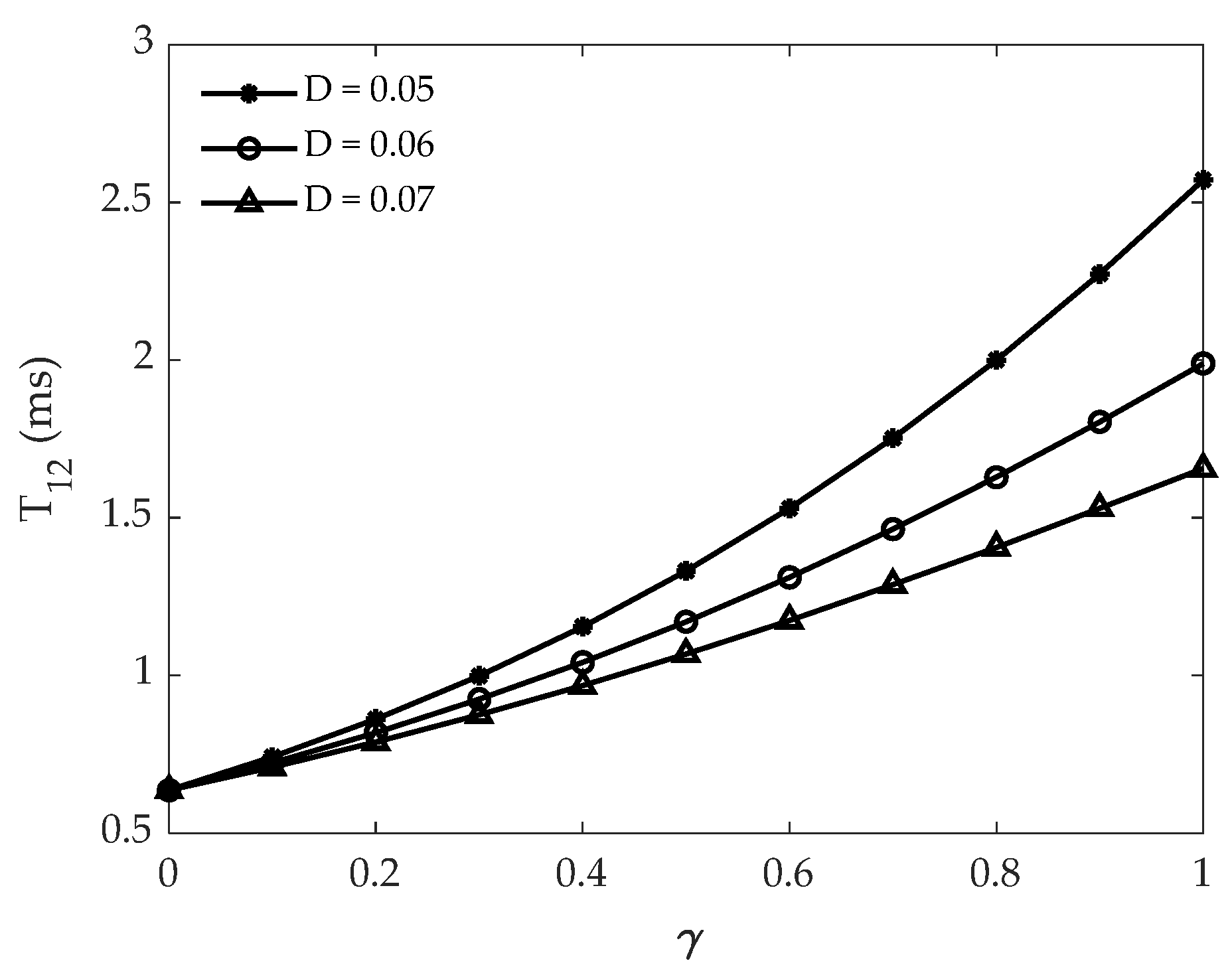
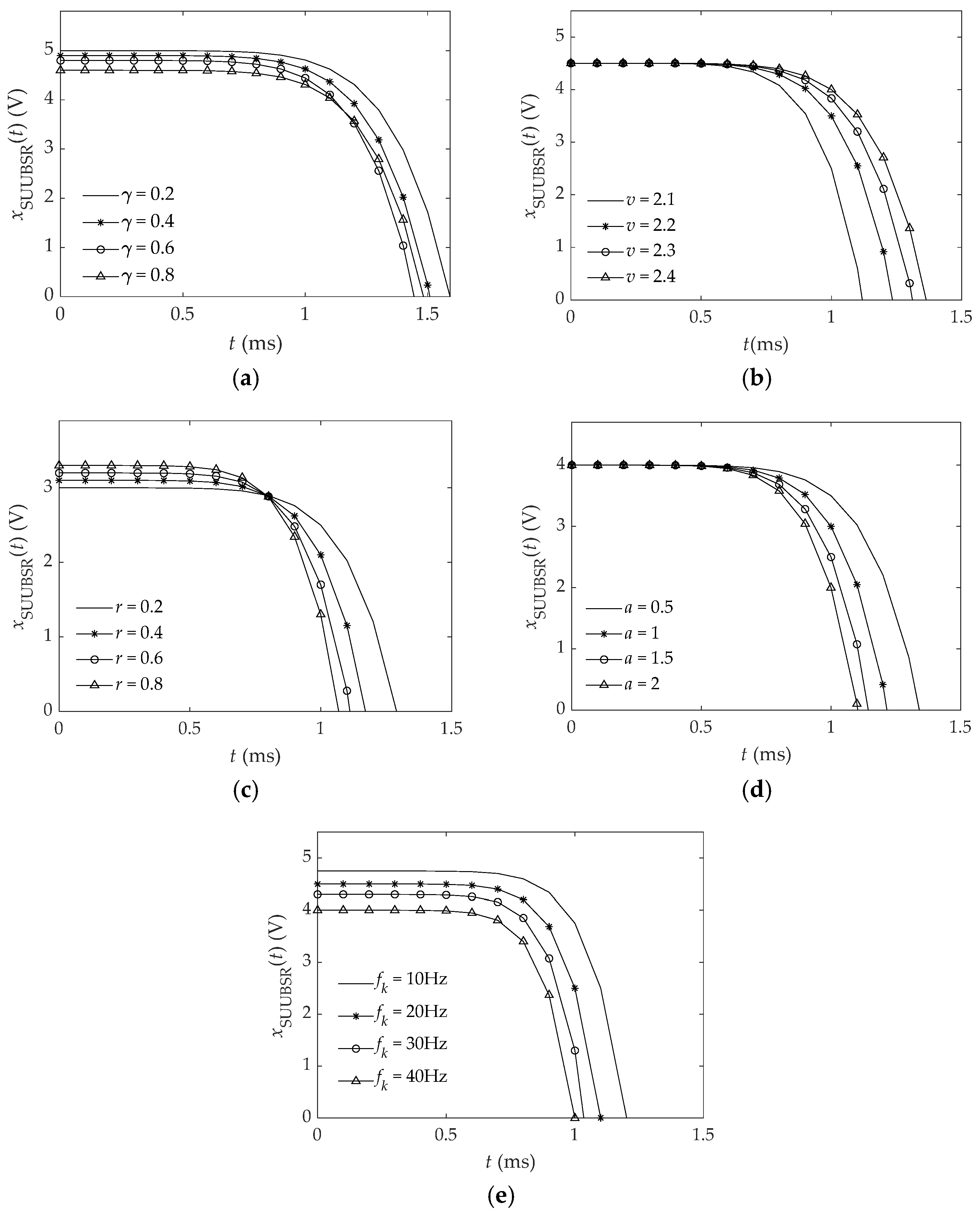
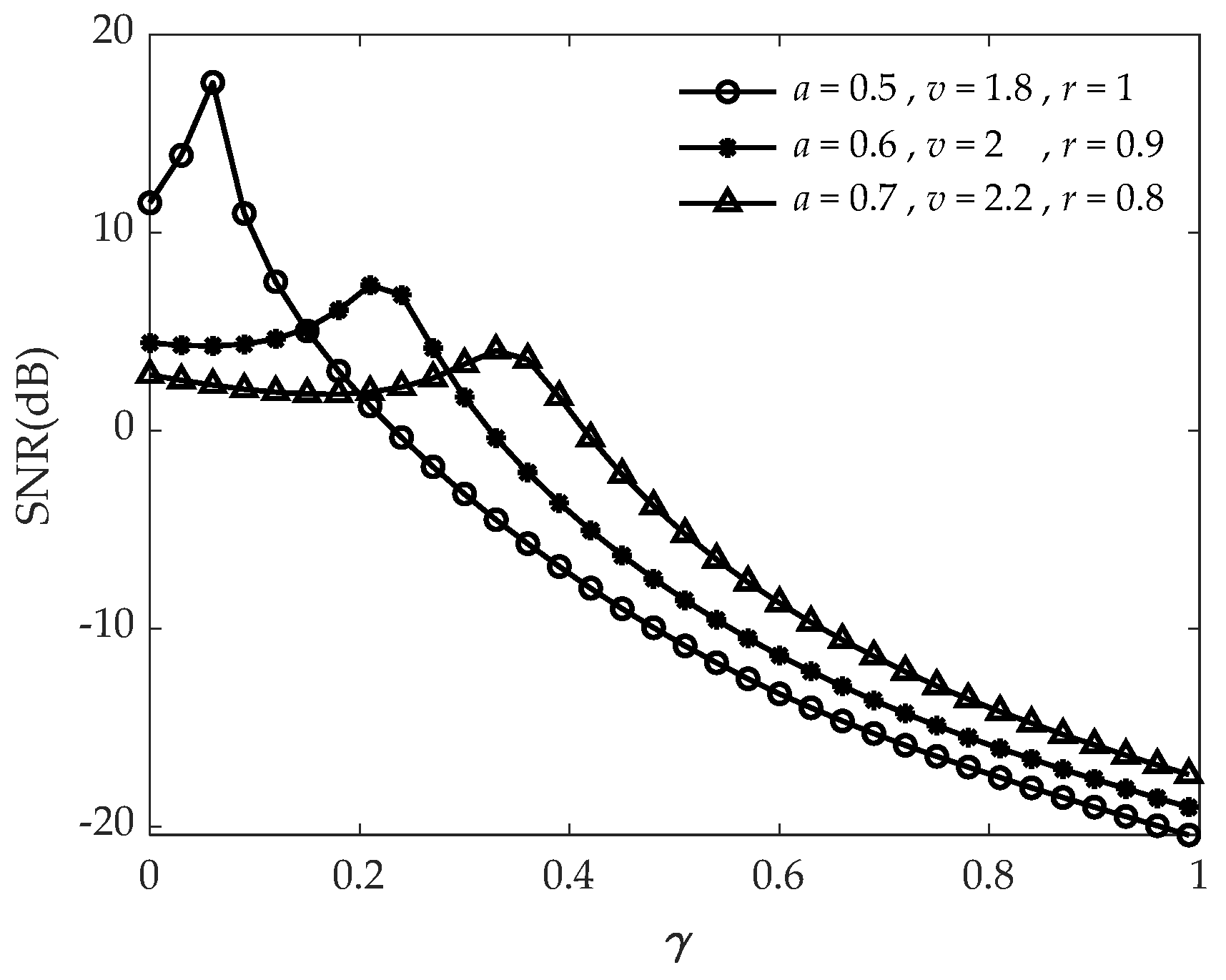
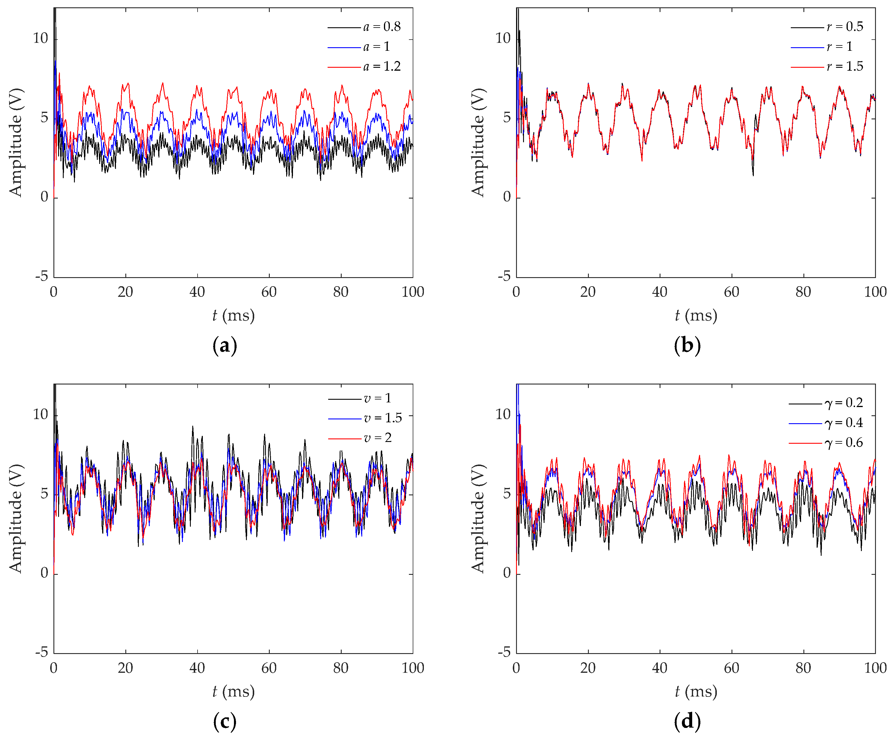
3.2.2. Influence of System Parameters and Input Signal Frequency on the System Response Speed

There are two main factors affecting the system response speed, one is the system parameters, and the other is the frequency of external input signals. In order to further explore the influencing factors of system response speed, this paper takes the exponential decay term in Formula (36) for analysis:

$$\begin{array}{l}{x}_{UUBSR}(t)=\ln \left({\displaystyle \frac{2v}{a{r}^2}}\right)e^{-{\displaystyle \frac{\gamma }{2}}t}{\displaystyle \sum _{k=0}^{N-1}\frac{2\pi f_k{\beta }_k\gamma (\sin {\theta }_k+R_{1,2}\cos {\theta }_k)}{4D{R_{1,2}}^2(1+\frac{{\pi }^2{f_k}^2}{{R_{1,2}}^2})\sqrt{(4b-{\gamma }^2)}}}\sin \left({\displaystyle \frac{\sqrt{4b-{\gamma }^2}}{2}}t\right)\\ +\ln \left({\displaystyle \frac{2v}{a{r}^2}}\right)e^{-{\displaystyle \frac{\gamma }{2}}t}{\displaystyle \sum _{k=0}^{N-1}\frac{r^2{\beta }_k\left(R_{1,2}\sin {\theta }_k-\cos {\theta }_k\right)}{2D{R_{1,2}}^2(1+\frac{{\pi }^2{f_k}^2}{{R_{1,2}}^2})}}\cos \left({\displaystyle \frac{\sqrt{4b-{\gamma }^2}}{2}}t\right)\end{array}$$

(39)

After combining and simplifying Formula (39), Formula (40) is obtained as follows:

$$x_{UUBSR}(t)=e^{-{\displaystyle \frac{\gamma }{2}}t}\sqrt{{\left(C_1\right)}^2+{\left(C_2\right)}^2}\sin \left({\displaystyle \frac{\sqrt{4b-{\gamma }^2}}{2}}t+\varphi \right)$$

(40)

where $\varphi =\arctan {\displaystyle \frac{r^2\left(R_{1,2}\sin {\theta }_k-\cos {\theta }_k\right)}{\pi f_k\gamma \left(\sin {\theta }_k+R_{1,2}\cos {\theta }_k\right)}}$.

By performing a Taylor series expansion on Formula (40), the Taylor series expansion of Formula (41) is obtained as follows:

$$x_{\mathrm{SUUBSR}}(t)=\sqrt{{\left(C_1\right)}^2+{\left(C_2\right)}^2}{\displaystyle \sum _{L=0}^{\infty }\frac{{(-1)}^{3L+1}{\gamma }^L{\left(\frac{\sqrt{4b-{\gamma }^2}}{2}t+\varphi \right)}^{2L+1}{t}^L}{2^{L}L!\left(2L+1\right)!}}$$

(41)

The influence diagram of system parameters and input signal frequency on the system response speed obtained from Formula (41) is shown in Figure 4. It can be seen from Figure 4a that the larger the damping coefficient value, the smaller the initial value of the transient response, and the faster the system response speed. When the damping coefficient value is too large, the system response speed becomes slow. In Figure 4c, as the parameter r increases, the initial value of the system transient response decreases, and the system response speed slows down. In Figure 4b,d, the parameters a and v do not affect the initial value of the transient response. As a increases, the system response speed becomes faster, and as v increases, the system response speed slows down. In Figure 4e, as the input signal frequency increases, the initial value of the transient response decreases, and the system response speed slows down.

Furthermore, an approximate functional expression between time $T_d$, $\gamma$, and input signal frequency $f_k$ can be obtained.

$$T_d=\sqrt[3L+1]{{\displaystyle \sum _{L=0}^{\infty }\frac{x_{si}{2}^{2L}L!\left(2L+1\right)!}{{(-1)}^{3L+1}{\gamma }^L\sqrt{{\left(4b-{\gamma }^2\right)}^{2L+1}}\sqrt{{\left(C_1\right)}^2+{\left(C_2\right)}^2}}}}$$

(42)

In Formula (42), L is a positive integer; in this case, $T_d>0$, and it can be seen from the formula that the transient response time is related to the damping coefficient, particle transition rate, and signal frequency. The higher the input signal frequency and the greater the particle transition rate, the shorter the transient response time of the system. Meanwhile, the relationship between the damping coefficient and the transient response time is not completely monotonic. When the damping coefficient is within the range of $\left(0,\sqrt{4b/3}\right)$, an increase in the damping coefficient leads to a shorter transient response time. However, when the damping coefficient is within the range of $\left(\sqrt{4b/3},1\right)$, an increase in the damping coefficient gradually exhibits an overdamping characteristic, resulting in a longer transient time and a slower response speed.

3.3. Steady-State Response Analysis

After a transient response of duration $T_d$, the system begins to enter a steady-state phase during which the particle moves within the initial trap. To solve for the steady-state output of the system, the generalized Langevin gradient equation is chosen to represent the steady-state output state equation of the system.

$${\displaystyle \frac{d^2{x}_{\mathrm{Q}}(t)}{d{t}^2}}+\gamma {\displaystyle \frac{d{x}_{\mathrm{Q}}(t)}{dt}}=f(x_{\mathrm{Q}}(t),t)+\epsilon (x_{\mathrm{Q}}(t),t)$$

(43)

In the equation, $f(x_{\mathrm{Q}}(t),t)$ is the deterministic component, and $\epsilon (x_{\mathrm{Q}}(t),t)$ is the external random force.

For the convenience of solving, Equation (43) can be rewritten into the form of Equation (44) based on statistical theory:

$${\displaystyle \frac{d^2{x}_{\mathrm{Q}}(t)}{d{t}^2}}+\gamma {\displaystyle \frac{d{x}_{\mathrm{Q}}(t)}{dt}}=f(x_{\mathrm{Q}}(t),t)+\mathit{G}{\nabla }_x\ln J(x_{\mathrm{Q}}(t),t)$$

(44)

where $\mathit{G}$ represents the diffusion matrix of the state vector in the state space, ${\nabla }_x$ represents the gradient operator, and $J(x_{\mathrm{Q}}(t),t)$ represents the Jacobian determinant, $\ln J(x_{\mathrm{Q}}(t),t)=-\ln \rho (x_{\mathrm{Q}}(t),t)$.

First, the deterministic component in Equation (44) is analyzed. Assuming that when the system initially reaches $x_{si}$$\left(i=1,2\right)$ steady-state condition, the particle is located near the steady-state point a of the SUUBSR system. The deterministic component is Taylor expanded at the two steady-state points, $x_{s1}$ and $x_{s2}$, of the nonsaturating potential function. Then, Taylor series expansions $f_1(x_{\mathrm{Q}}(t),t)$ and $f_2(x_{\mathrm{Q}}(t),t)$ are obtained, which can be expressed as follows:

$$\begin{array}{l}{f}_i(x_{\mathrm{Q}}(t),t)={\displaystyle \sum _{j=1}^n{a}_{ij}(t)x_j(t)+{\displaystyle \sum _{j_1=1}^n{\displaystyle \sum _{j_2=1}^n{a}_{i{j}_1{j}_2}(t){x_{\mathrm{Q}}}_{j_1}(t){x_{\mathrm{Q}}}_{j_2}(t)}}}+\cdots \\ +{\displaystyle \sum _{j_1=1}^n{\displaystyle \sum _{j_2=1}^n\cdots {\displaystyle \sum _{j_s=1}^n{a}_{i{j}_1{j}_2\cdots j_s}(t){x_{\mathrm{Q}}}_{j_1}(t){x_{\mathrm{Q}}}_{j_2}(t)\cdots {x_{\mathrm{Q}}}_{j_s}(t)}}+\cdots }\end{array}$$

(45)

where $x_j(t)$ represents the Taylor expansion term at the expected value point $x_{si}$ of the SUUBSR system.

For ease of writing, Equation (43) can be written as follows:

$${\displaystyle \frac{d^2{x}_{\mathrm{Q}}(t)}{d{t}^2}}+\gamma {\displaystyle \frac{d{x}_{\mathrm{Q}}(t)}{dt}}=\mathit{A}(t)x_{\mathrm{Q}}(t)+\psi (x_{\mathrm{Q}}(t),t)+\mathit{G}{\nabla }_x\ln J(x_{\mathrm{Q}}(t),t)$$

(46)

In the equation, $\mathit{A}(t)={[a_{ij}(t)]}_{n\times n}$ is a matrix of size $n\times n$, and $\psi (x_{\mathrm{Q}}(t),t)$ represents the higher-order terms in the equation $f_i(x_{\mathrm{Q}}(t),t)$.

Assuming that the stochastic resonance system driven by the current OFDM signal has entered the steady-state response phase, and the duration of the steady-state response is one period of the OFDM signal, the output state equation is solved using the successive approximation method to obtain the following solution:

$$\begin{array}{l}{x}_{\mathrm{Q}}(t)=(1+\gamma )\mathit{R}(t)x_{\mathrm{Q}}(0)+\mathit{R}(t){\displaystyle {\int }_{T_d}^{T_s}{\mathit{R}}^{-1}(\tau )}\phi (x_{\mathrm{Q}}(\tau ),\tau )d\tau \\ +\mathit{R}(t){\displaystyle {\int }_{T_d}^{T_S}{\mathit{R}}^{-1}(\tau )\mathit{G}{\nabla }_x\ln J(x_{\mathrm{Q}}(\tau ),\tau )d\tau }\end{array}$$

(47)

where $R(t)$ is the solution to the equation ${\displaystyle \frac{d{x}_{\mathrm{Q}}(t)}{dt}}=\mathit{A}(t)x_{\mathrm{Q}}(t)$, the initial value is $\mathit{R}(0)=\mathrm{E}$, $\mathrm{E}$ is an identity matrix of size $n\times n$, and the general form of $\mathit{R}(t)$ is as follows:

$$\begin{array}{l}\mathit{R}(t)=E+{{\displaystyle \int }}_0^t\mathit{A}\left(t_1\right)\mathrm{d}{t}_1+{{\displaystyle \int }}_0^t{{\displaystyle \int }}_0^{t_1}\mathit{A}\left(t_1\right)\mathit{A}\left(t_2\right)\mathrm{d}{t}_1\mathrm{d}{t}_2+\cdots \\ +{{\displaystyle \int }}_0^1{{\displaystyle \int }}_0^{t_1}\cdots {{\displaystyle \int }}_0^{t_{n-1}}\mathit{A}\left(t_1\right)\mathit{A}\left(t_2\right)\cdots \mathit{A}\left(t_n\right)\mathrm{d}{t}_1\mathrm{d}{t}_2\cdots \mathrm{d}{t}_{n-1}\mathrm{d}{t}_n\cdots \end{array}$$

(48)

According to Formula (47) and (48), when the particle passes through the left and right stable points during the transition process, DC bias components with a magnitude of $\left(1+\gamma \right)x_{si}$ will be generated at the left and right stable points. During a complete inter-trap stochastic resonance motion of the particle, due to the symmetry of the potential function, the positive and negative DC bias components generated at the positive and negative potential wells cancel each other out, so the DC bias component will not affect the steady-state output value of the system. At this time, under the steady-state limit condition of the system, when $t_0\to T_s$, the expression of the autocorrelation function of the steady-state response of the system is obtained as follows:

$$\begin{array}{l}\underset{t_0\to T_s}{\lim }〈x_{\mathrm{Q}}\left(t+\tau \right)x_{\mathrm{Q}}\left(t\right)|x_{\mathrm{Q}}\left(0\right),t_0〉=〈x_{\mathrm{Q}}\left(t+\tau \right)x_{\mathrm{Q}}\left(t\right)〉\\ =x_{si}^2\exp \left(-2R_{1,2}\left|\tau \right|\right)\left[1-\kappa {\left(t\right)}^2\right]+x_{si}^2\kappa \left(t+\tau \right)\kappa \left(t\right)\end{array}$$

(49)

where $\kappa \left(t\right)$ can be described as follows:

$$\kappa \left(t\right)={\displaystyle \sum _{k=0}^{K-1}\frac{2R_{1,2}{\beta }_k{x}_{s_i}\sin \left(w_{k}t+{\theta }_k\right)}{D\sqrt{4{R_{1,2}}^2+{w_k}^2}}}$$

(50)

The time-domain average of the autocorrelation function of the steady-state output of the system excited by an OFDM signal with a single symbol period is obtained as follows:

$$\begin{array}{l}〈〈x_{\mathrm{Q}}\left(t\right)x_{\mathrm{Q}}\left(t+\tau \right)〉〉={\displaystyle \frac{1}{T_s}}{\displaystyle {\int }_{T_d}^{T_s}〈x_{\mathrm{Q}}\left(t\right)x_{\mathrm{Q}}\left(t+\tau \right)〉}dt={\displaystyle \sum _{k=0}^{K-1}{x}_{si}^2\exp \left(-2R_{1,2}\left|\tau \right|\right)}\\ \left[1-{\displaystyle \frac{1}{2}}{\left({\displaystyle \frac{{\beta }_k{x}_{s_i}}{D}}\right)}^2{\displaystyle \frac{4R_{1,2}^2}{4R_{1,2}^2+{w_k}^2}}\right]+{\displaystyle \sum _{k=0}^{K-1}\frac{x_{si}^2}{2}}{\left({\displaystyle \frac{{\beta }_k{x}_{s_i}}{D}}\right)}^2{\displaystyle \frac{4R_{1,2}^2}{4R_{1,2}^2+{w_k}^2}}\cos \left(w_k\tau +{\theta }_k\right)\end{array}$$

(51)

Performing a Fourier transform on Equation (51) yields the analytical expression for the power spectrum of the steady-state output of the system:

$$\begin{array}{l}X\left(w\right)=X_N\left(w\right)+X_S\left(w\right)={\displaystyle \sum _{k=0}^{K-1}\left[1-\frac{1}{2}{\left(\frac{{\beta }_k{x}_{s_i}}{D}\right)}^2\frac{4R_{1,2}^2}{4R_{1,2}^2+{w_k}^2}\right]}{\displaystyle \frac{4R_{1,2}^2{x}_{si}^2}{4R_{1,2}^2+w^2}}+\\ {\displaystyle \sum _{k=0}^{K-1}\frac{\pi }{2}}{\left({\displaystyle \frac{{\beta }_k{x}_{si}}{D}}\right)}^2{\displaystyle \frac{4R_{1,2}^2}{4R_{1,2}^2+{w_k}^2}}\left[\delta \left(w-w_k\right)+\delta \left(w+w_k\right)\right]\end{array}$$

(52)

The steady-state output SNR is the ratio of the total signal power at each subcarrier frequency of the system output signal to the total noise power at each subcarrier frequency when the system reaches a steady state. Its expression is as follows:

$$\left\{\begin{array}{l}SNR={\displaystyle \frac{P_s}{{\displaystyle \sum _{k=0}^{K-1}{X}_N\left(w_k\right)}}}\\ P_s=\underset{\Delta w\to 0}{\lim }{\displaystyle \sum _{k=0}^{K-1}{\displaystyle {\int }_{w_k-\Delta w}^{w_k+\Delta w}{X}_S\left(w\right)dw}}\end{array}\right.$$

(53)

The steady-state output SNR expression of the SUUBSR system is derived from Equation (53):

$$SNR={\displaystyle \sum _{k=0}^{K-1}\frac{R_{1,2}\pi {A_k}^2{r}^2\ln \left(\frac{2v}{a{r}^2}\right)}{2}{\left[1-\frac{4R_{1,2}^2{r}^2{A_k}^2\ln \left(\frac{2v}{a{r}^2}\right)}{2D^2\left(4R_{1,2}^2+{w_k}^2\right)}\right]}^{-1}}$$

(54)

Based on Equation (54), a relationship curve between the steady-state output SNR and the damping coefficient under different parameters is plotted as shown in Figure 5. As can be observed from Figure 5, under the same damping coefficient, the smaller v is, the larger a and r are, and the higher the peak of the signal–noise ratio curve will be. This indicates that a lower potential barrier in the potential function favors particle transitions. When the system parameters remain constant, the value of the steady-state output SNR first increases and then decreases with the increase in the damping coefficient, showing that there is not a monotonic relationship between the damping coefficient and the SNR value. Instead, there exists an optimal damping coefficient that optimizes the value of the steady-state output SNR.

4. Experimental Simulation

4.1. Detection Simulation of Communication Signal Waveform by FUBSR and SUUBSR

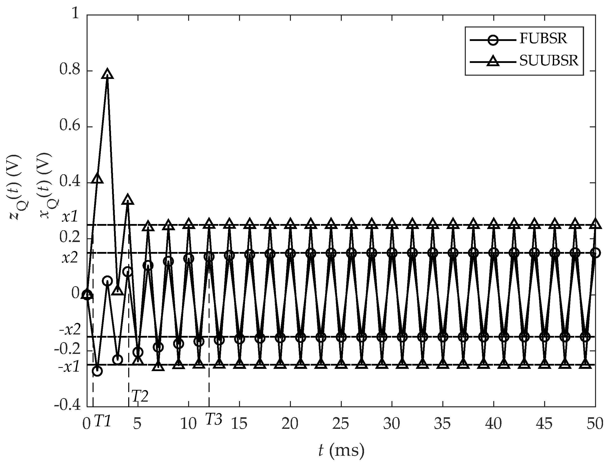
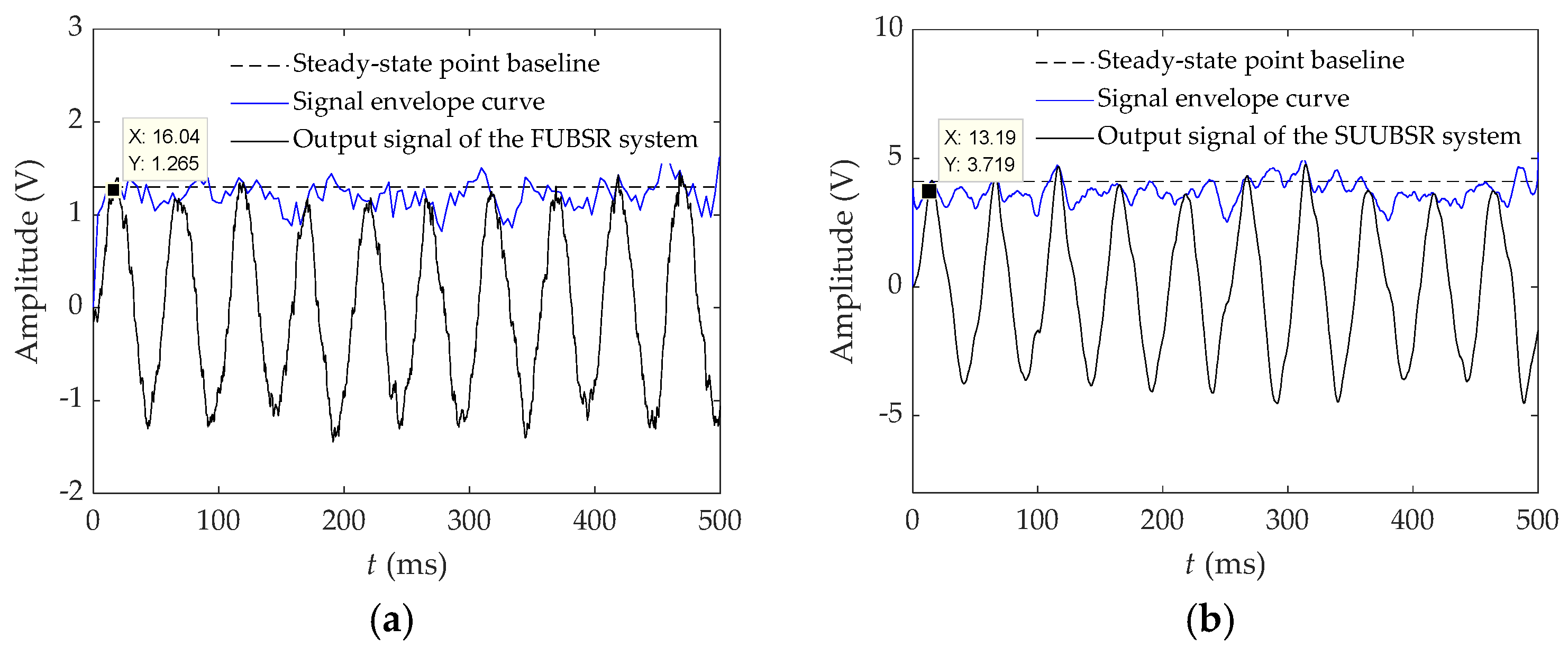
4.1.1. Detection Simulation of Single-Carrier Signal Waveform by FUBSR and SUUBSR

Through experimental simulation, the detection effects of SUUBSR and FUBSR systems on single-carrier signal waveforms under high background noise were tested. The simulation parameter settings were as follows: the input signal $s_{\mathrm{Q}}(t)=Q_m\sin \left(2\pi f_{c}t+{\theta }_c\right)$ was the quadrature component of a single-carrier signal; $Q_m$ was the imaginary part of the complex value mapped by the binary data stream after 16 QAM modulation; carrier frequency $f_c=10\mathrm{Hz}$; carrier phase ${\theta }_c=\pi /4$; noise intensity $D=1$; and quantum particle swarm optimization was used to optimize the parameters of the FUBSR system and the SUUBSR system to obtain the optimal parameter combination of $a=0.7793$, $v=4.2755$, and $r=3.4298$; $a=0.0973$, $v=0.6391$, $r=4.8007$, and $\gamma =0.9030$; sampling frequency $f_s=4.55\mathrm{Hz}$; and sampling step size $h=1/f_s$.

Figure 6 presents the detection results of the FUBSR and SUUBSR systems for the waveform of a faint single-carrier signal, respectively. It can be observed from the figure that both systems can enhance the faint single-carrier signal. The output signal of the SUUBSR system has a higher amplitude value and fewer spikes caused by noise interference, indicating that the SUUBSR system has better noise resistance. From the perspective of the upper envelope curves of the output signals of the two systems, the FUBSR system enters a steady state at 3.38% of the symbol period, while the SUUBSR system enters a steady state within 1.93% of the symbol period, demonstrating that the SUUBSR system has a faster response speed.

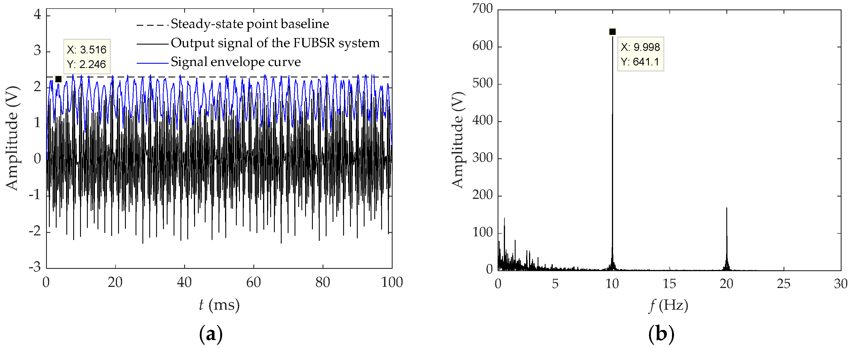
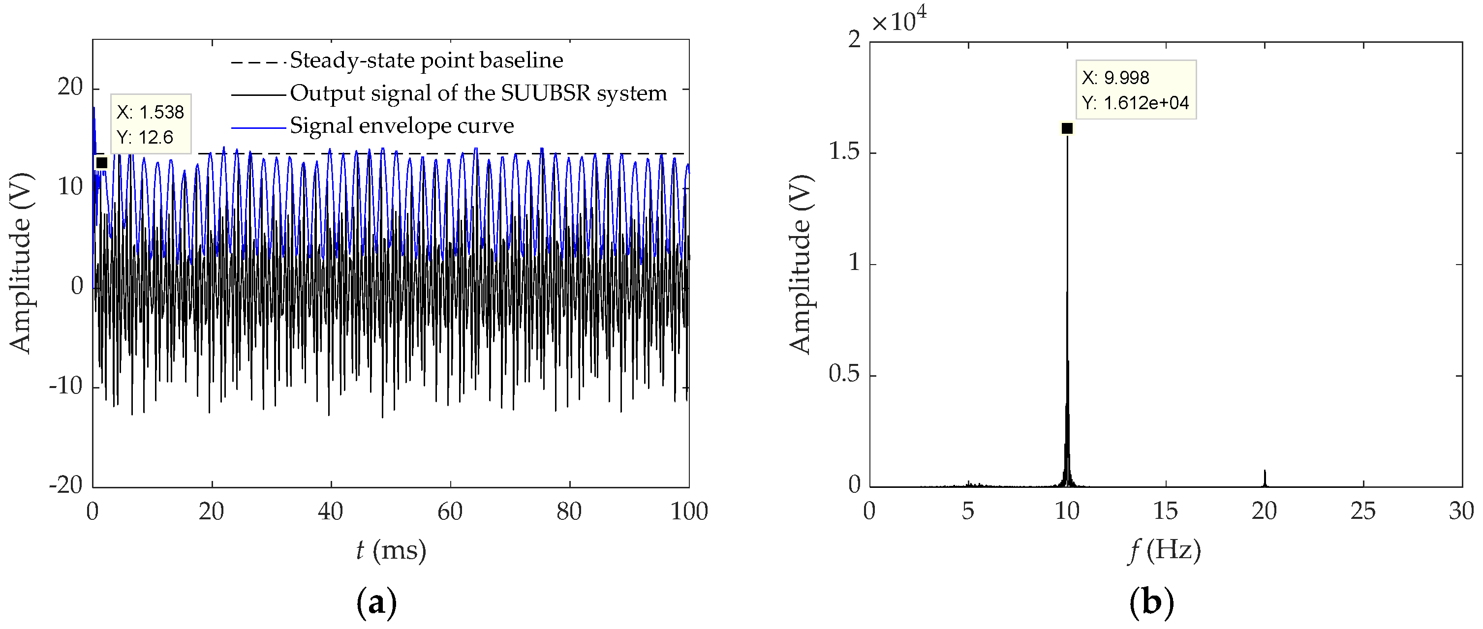
4.1.2. Simulation of Detection of OFDM Signal Waveforms by FUBSR Stochastic Resonance and SUUBSR Systems

The following is an experimental simulation of the detection effect of FUUBSR and UBSR systems on weak OFDM signals under high background noise. Take the signal $s_{\mathrm{Q}}(t)={\displaystyle {\sum }_{k=0}^{K-1}{\beta }_k}\sin \left(2\pi f_{k}t+{\theta }_k\right)$, the number of subcarriers $K=2$, the carrier spacing $\Delta f=10 \mathrm{Hz}$, individual carrier frequencies $f_{1,2}=\left[10,20\right]$ Hz, individual carrier phases ${\theta }_{1,2}=[0,\pi /2]$, and noise intensity $D=1$. Let the sampling frequency $f_s=4000 \mathrm{Hz}$, and the sampling step size $h=1/f_s$, through the use of a quantum particle swarm optimization algorithm to optimize the parameters of the FUBSR system and SUUBSR system, the optimal parameter combination is obtained as $a=3.51,v=2.8493,r=1.835$; $a=1.2306$, $v=0.778$, $r=1.389$, and $\gamma =0.63$.

As can be seen from Figure 7a,b, the upper envelope line of the FUBSR system output signal reaches the system steady-state value point at 3.516% of the symbol period. The amplitude in the time–frequency domain is significantly improved compared to the original noisy signal, and the output SNR is −1.6753 dB. The irregularity of the upper envelope waveform indicates that the time-domain waveform is still greatly affected by the background noise, and the burrs on the waveform have not been weakened. This shows that the nonsaturation model can effectively enhance the amplitude of weak signals, but it cannot solve the poor anti-noise performance of the first-order system.

From Figure 8a,b, it can be seen that the SUUBSR system output signal reaches the system steady-state value point at 1.538% of the symbol period with an output SNR of −0.0256 dB. The amplitude in the output time–frequency domain has been significantly enhanced, far higher than the enhancement effect of the FUBSR system on weak OFDM signals. After reaching the steady state, the upper envelope waveform is regular, and the burrs on the time-domain waveform have basically disappeared. This indicates that the SUUBSR system has better anti-noise performance and faster system response speed compared to the FUBSR system.

The envelope can better reflect the changing trend of signal amplitude. By observing the change in the envelope, the response speed of the system can be analyzed. Figure 9 shows the changing trend of the output signal envelope of the SUUBSR system under different system parameters. In Figure 9a, as the system parameter a increases, the envelope amplitude value increases, and the oscillation slope increases, indicating that the system response speed becomes faster and the signal enhancement effect becomes better. In Figure 9b, the parameter r only affects the oscillation slope of the envelope and has little effect on the envelope amplitude. The smaller the parameter r, the faster the system response speed is. In Figure 9c, as v increases, the envelope amplitude and oscillation slope both decrease, and the system response speed slows down. In Figure 9d, when the damping coefficient is too small, the envelope oscillation slope becomes smaller, and the envelope also oscillates due to the system oscillation. As the damping coefficient increases, the envelope slope increases, and the envelope waveform is more regular, indicating that increasing the damping coefficient within a certain range can speed up the system response speed and increase the system stability.

4.2. Performance Analysis of OFDM Signal Demodulation

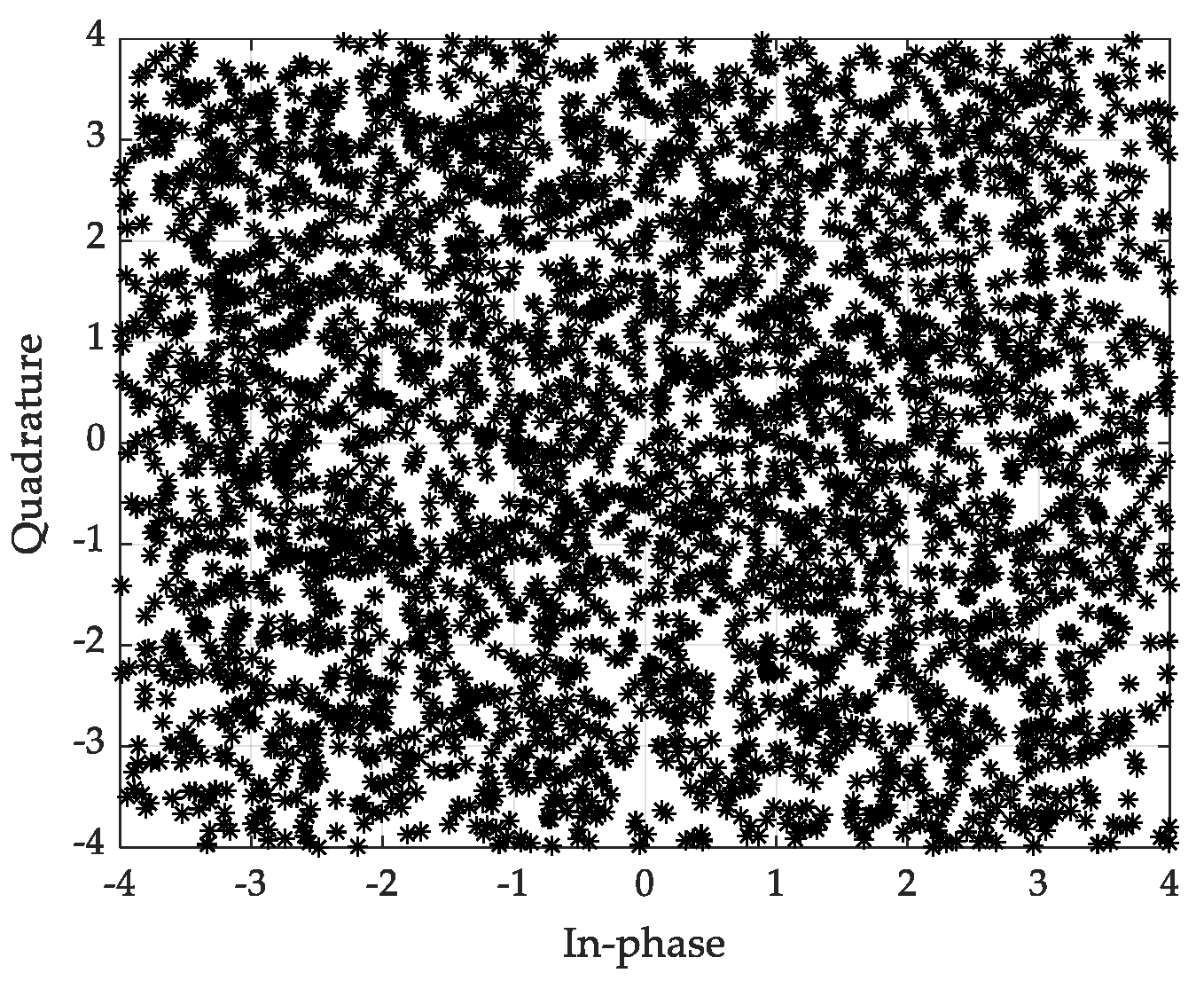
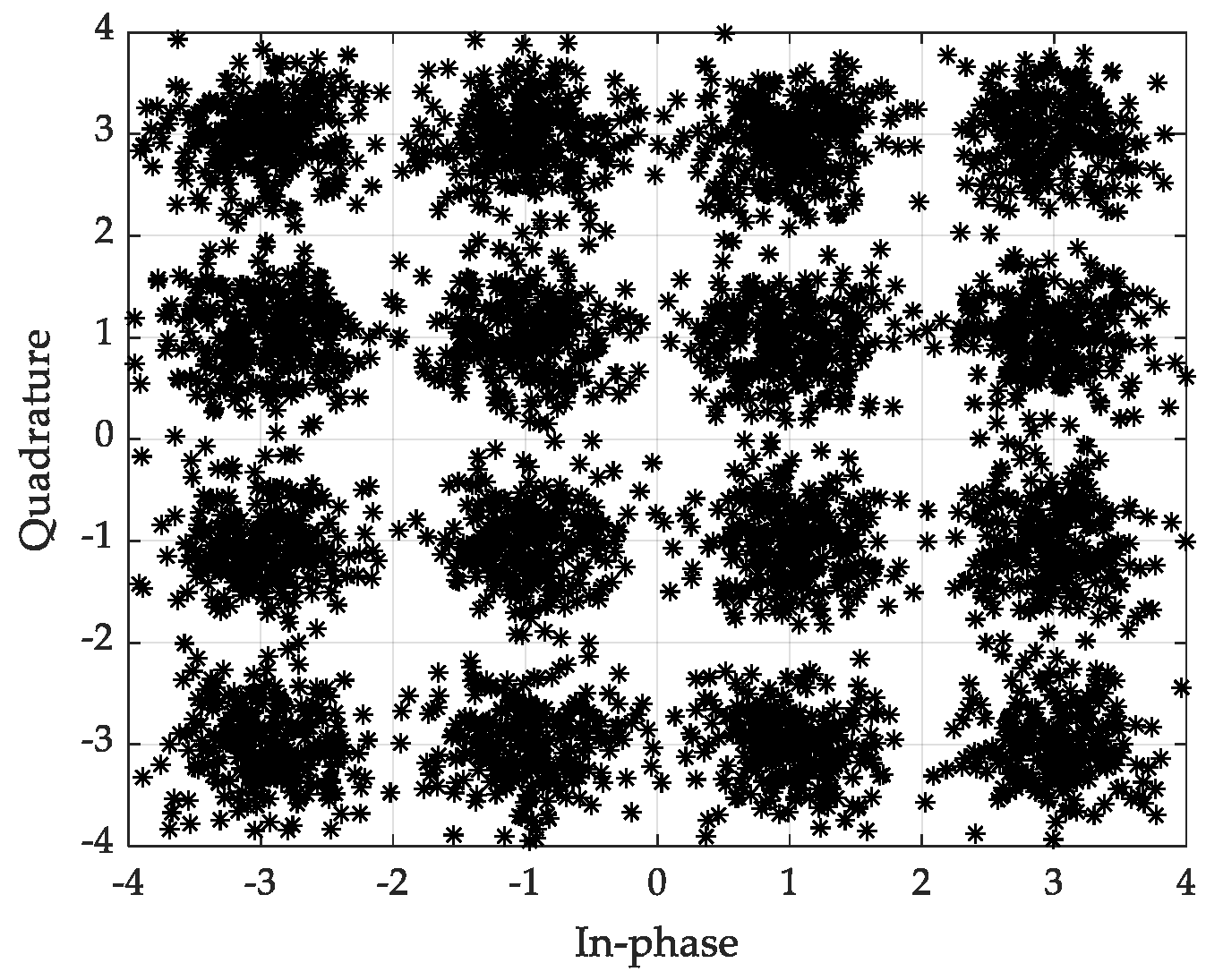
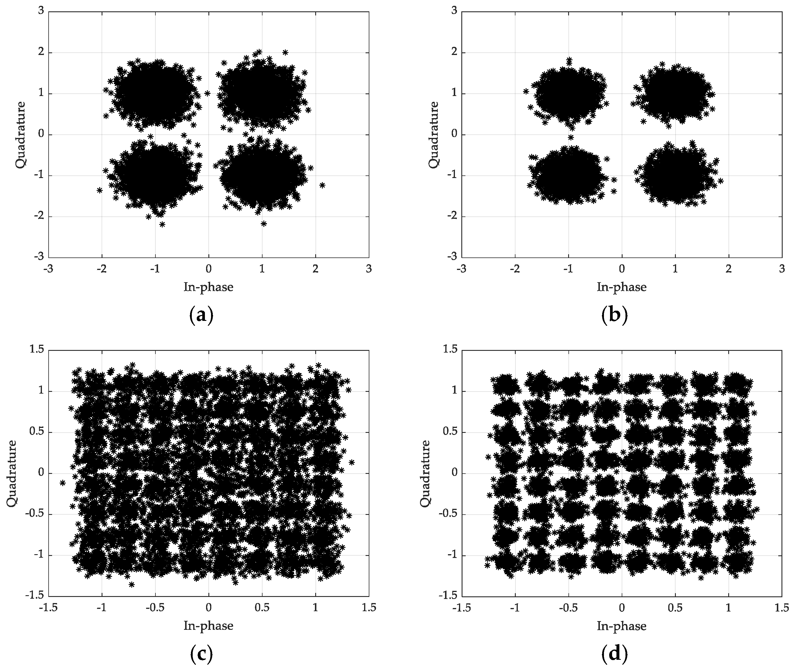
4.2.1. Simulation of Demodulation Process of OFDM Signals by FUBSR and SUUBSR Systems

To further verify the demodulation effect of OFDM signals in the FUBSR and SUUBSR systems, as well as the integration of these two systems with the OFDM signal demodulation process, constellation diagrams at the receiver end of different stochastic resonance systems are plotted under the condition of an SNR of 2 dB. The demodulation performance of the system for OFDM signals is analyzed by examining the deviation of each point in the constellation diagram from the central position. The simulation parameters are set as follows: the number of subcarriers is 64, the number of OFDM signal symbols is 20, and the modulation method is 16 QAM. Under the condition of an SNR of 2 dB, using the quantum particle swarm optimization algorithm, the optimal parameter sets $a=4.71,v=3.3493,r=1.6614$; $a=1.1,v=0.4161,r=1.6,\gamma =0.511$, for the two systems are obtained by optimizing the system parameters based on the OFDM signal SNR as the evaluation metric. The constellation diagrams before and after the demodulation of the OFDM signal processed by the FUBSR system under 16 QAM modulation are shown in Figure 10 and Figure 11.

Figure 10 shows the constellation diagram of the OFDM signal after passing through a Gaussian channel. As can be seen from Figure 10, due to the influence of Gaussian noise, the constellation diagram of the OFDM signal becomes very chaotic. Figure 11 depicts the constellation diagram of the OFDM signal demodulated by the FUBSR system. Compared to Figure 10, the points in Figure 11 are more concentrated around the 16 initial central points, indicating that the FUBSR system can be combined with the demodulation process of OFDM signals. However, there are still many points deviating, indicating that the demodulation effect is not ideal.

Figure 12 shows the constellation diagram of the OFDM signal demodulated by the SUUBSR system proposed in this paper. Most of the points in Figure 12 are clustered around the 16 initial central points, with only a small number of points deviating. This indicates that the demodulation performance of the SUUBSR system for OFDM signals is better than that of the FUBSR system.

To further verify the demodulation performance of the proposed system in this paper for OFDM signals under different subcarrier modulation schemes, the simulation parameters are kept consistent with those for 16 QAM subcarrier modulation. The FUBSR system and the SUUBSR system are used to demodulate and simulate OFDM signals with QPSK and 64 QAM modulation schemes. The constellation diagrams of the OFDM signals processed by the FUBSR system and the SUUBSR system after demodulation, under QPSK and 64 QAM subcarrier modulation schemes, are shown in Figure 13. From Figure 13, it can be observed that under both QPSK and 64 QAM subcarrier modulation schemes, the constellation diagrams of the OFDM signals processed by the SUUBSR system exhibit better clustering than those processed by the FUBSR system.

4.2.2. Demodulation Effect of OFDM Signals in Different Stochastic Resonance Systems

After verifying the superiority of the demodulation performance of the proposed SUUBSR system compared to the FUBSR system, the following discussion will focus on the impact of the damping coefficient on the demodulation performance of the system. The analysis method adopted is to fix the noise intensity and system parameters while only varying the value of the damping coefficient. By observing the deviation degree of the constellation points at the system output end compared to the initial 16 points, the influence of the damping coefficient and noise intensity on the demodulation effect of OFDM signals can be analyzed. The simulation parameters are set as follows: the number of subcarriers is 64; the number of OFDM signal symbols is 20, taking 16 QAM modulation as an example; and the fixed system parameters are $a=0.2306$, $v=0.4398$, and $r=3.5615$.

Let D = 100, and the damping coefficient values are set to 0.5, 0.6, 0.7, and 1 sequentially. The demodulation constellation diagrams of OFDM signals corresponding to each damping coefficient value are plotted in Figure 14. As can be seen from Figure 14, when the damping coefficient value exceeds the critical damping value, with the increase in the damping coefficient, the data points of the OFDM signal in the constellation diagram tend to cluster around the initial 16 points first and then gradually deviate. The demodulation effect of the damping coefficient above the critical damping is significantly better than that of the damping coefficient below the critical damping. However, the value of the damping coefficient is not necessarily better as it increases, but rather has a certain range. Only when the optimal damping coefficient value is achieved will the anti-noise performance of the SUUBSR system and the demodulation effect of the OFDM signal be improved.

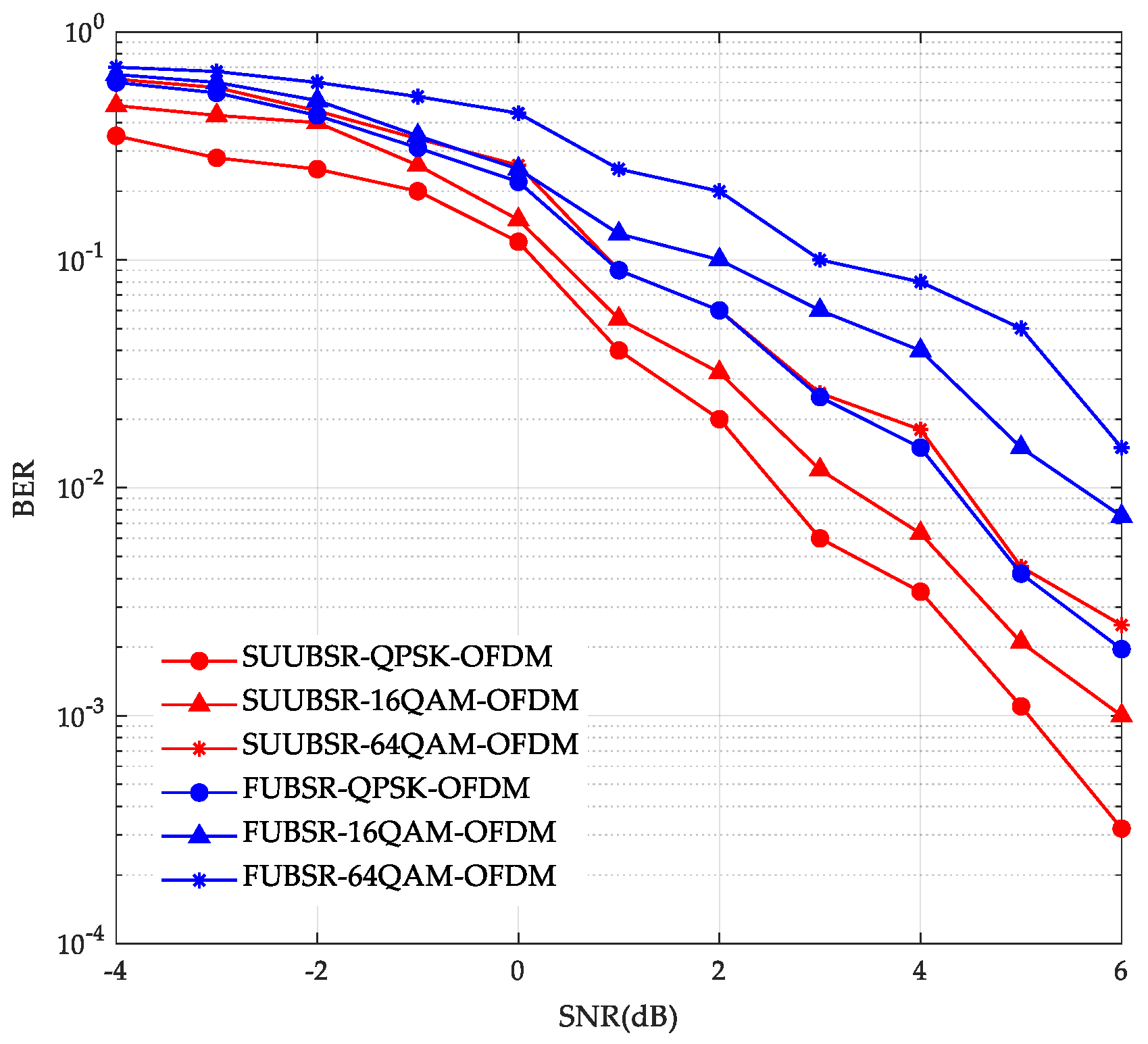
4.3. System Bit Error Rate Analysis

The following further validates the conclusions drawn above through the system’s bit error rate (BER). BER curves for OFDM signals demodulated by the FUBSR system and the SUUBSR system under different subcarrier modulation schemes were plotted within an SNR range of −4 to 6 dB, as shown in Figure 15. From Figure 15, it can be observed that as the SNR increases, both systems can improve the demodulation performance of OFDM signals with different modulation schemes, and the demodulation effect is better for OFDM signals modulated with QPSK than for those modulated with 16 QAM and 64 QAM. During the demodulation process of OFDM signals with different subcarrier modulation schemes, the system proposed in this paper demonstrates significantly superior demodulation performance compared to the FUBSR system, especially for the 64 QAM modulation scheme, which requires a higher noise environment, where the proposed system exhibits stronger noise resistance and demodulation effectiveness. In summary, the system proposed in this paper can achieve the enhancement and demodulation of OFDM signals with different subcarrier modulation schemes, demonstrating universality. Furthermore, under the same SNR conditions, it has a lower BER compared to the FUBSR system, providing advantages in terms of demodulation performance for OFDM signals.

4.4. Algorithm Complexity Analysis

To assess the complexity of an algorithm, one needs to consider the number of multiplication and addition operations performed within the algorithm. The computational complexity of the method proposed in this paper is primarily composed of three parts: the Runge–Kutta algorithm for the stochastic resonance system, the quantum particle swarm optimization algorithm, and FFT. When the system proposed in this paper processes an OFDM signal with one symbol period, the number of sampling points is n, and the maximum number of iterations for the quantum particle swarm algorithm is I. The number of real multiplication and addition operations required to implement the enhancement and demodulation process of an OFDM signal with one symbol period using the two systems is shown in

Table 1. Comparison of computational complexity between the two systems.

System	Number of Multiplications	Number of Additions
FUBSR	$(133I+40)n+2n(1+I){\log }_{2}n$	$n(22+18I)+7I+3(I+1){\log }_{2}n$
SUUBSR	$(201I+67)n+2n(1+I){\log }_{2}n$	$n(27+45I)+2I+(I+1)3n\log (2n)$

. From Table 1, it can be observed that compared to the OFDM signal enhancement and demodulation method based on the FUBSR system, the proposed method has a higher computational complexity but achieves better enhancement and demodulation performance as well as improved noise resistance.

5. Conclusions

In this paper, a second-order underdamped system is applied to the enhancement and demodulation of OFDM signals. A method for enhancing and demodulating OFDM signals based on SUUBSR is proposed. The expressions for the first passage time, transient, and steady-state responses of the system driven by OFDM signals are derived, respectively. It is found that the existence of a transient response can lead to energy loss in OFDM. The output response analytical expressions of the FUBSR system and the SUUBSR system are analyzed, theoretically proving that the response speed of the SUUBSR system is superior to that of the FUBSR system. The relationship between system parameters, damping coefficient, input signal frequency, and system response speed and transient response is explored. It is found that the above parameters have an impact on both the magnitude of the system’s transient response and its response speed. Larger values of parameters a and f_k result in shorter transient processes, while larger values of parameters v and r lead to longer transient processes. The damping coefficient is not linearly related to the length of the transient process, indicating that selecting appropriate parameters can minimize the impact of transient response on OFDM signals. During the steady-state response analysis, it is found that there is no DC offset component in the system that affects the steady-state output, and there exists an optimal damping that maximizes the steady-state output SNR. The simulation results show that the proposed system can eliminate the transient response of the system and enhance and demodulate OFDM signals with different subcarrier modulations such as QPSK, 16 QAM, and 64 QAM. Compared to the FUBSR system, the proposed system demonstrates better enhancement of weak OFDM signals, lower demodulation bit error rate, faster system response speed, and better noise resistance in low SNR environments.

As the noise environment in current communication systems becomes increasingly complex, this paper only discusses and analyzes the system performance of the proposed system in Gaussian white noise environments. Therefore, for future research work on this paper, the first priority should be to comprehensively consider the system’s ability to enhance and demodulate OFDM signals in different types of noise environments. Secondly, the objects processed by the proposed system should not be limited to communication signals. In the future, the system’s good noise resistance can be utilized for image processing. Finally, increasing the system order means increased computational complexity, so future research should also focus on how to reduce computational complexity.

References

1. Ji, C.; Zhao, Q.; Yu, Y.; Dai, W. Detection of Weak Signals Under Low SNR Stochastic Resonance System. IEEE Access 2023, 11, 101881–101889. [Google Scholar] [CrossRef]
2. Gao, R.; Jiao, S.; Xue, Q. Research and application of composite stochastic resonance in enhancement detection. Chin. Phys. B 2024, 33, 37–46. [Google Scholar] [CrossRef]
3. Ma, Z.; Jin, Y. Stochastic resonance in periodic potential driven by dichotomous noise. Acta Phys. Sin. 2015, 64, 84–90. [Google Scholar] [CrossRef]
4. Ding, J.; Guo, Y.; Mi, L. The transient characteristics of an underdamped periodic potential system excited by two different kinds of noise. Probabilistic Eng. Mech. 2023, 72, 103450. [Google Scholar] [CrossRef]
5. Zhang, C.; Lai, Z.; Tu, Z.; Liu, H. Stochastic resonance induced weak signal enhancement in a second-order tri-stable system with single-parameter adjusting. Appl. Acoust. 2024, 216, 109753. [Google Scholar] [CrossRef]
6. Zhai, Y.; Fu, Y.; Kang, Y. Incipient Bearing Fault Diagnosis Based on the Two-State Theory for Stochastic Resonance Systems. IEEE Trans. Instrum. Meas. 2023, 72, 1–11. [Google Scholar] [CrossRef]
7. Jin, Y.; An, Y. Weak Bearing Fault Diagnosis Based on Improved Stochastic Resonance of the Multi-Stable System. Trans. Beijing Inst. Technol. 2024, 44, 447–457. [Google Scholar] [CrossRef]
8. Li, M.; Shi, P.; Zhang, W.; Han, D. A novel underdamped continuous unsaturation bistable stochastic resonance method and its application. Chaos Solitons Fractals 2021, 151, 111228. [Google Scholar] [CrossRef]
9. Liu, G.; Peng, L. Research on the Application of Random Resonance in Three Stable Traps in Weak OFDM Signal Detection. Acta Metrol. Sin. 2023, 44, 1872–1881. [Google Scholar]
10. Liu, G.; Liang, Y. Research on OFDM signal detection method based on random resonance in bistable well. J. Syst. Simul. 2022, 34, 2046–2055. [Google Scholar] [CrossRef]
11. Wang, X.; Xiong, X.; Li, C.; Wu, B.; Niu, L. Impact of potential function asymmetry on the performance of a novel stochastic resonance system. Chin. J. Phys. 2024, 91, 11–24. [Google Scholar] [CrossRef]
12. Shu, Y.; Shen, J.; Lin, Y. Early Weak Fault Signal Enhancement and Recognition Method of Rudder Paddle Bearings Based on Parameter Adaptive Stochastic Resonance. IEEE Access 2024, 12, 9458–9467. [Google Scholar] [CrossRef]
13. Fu, Y.; Kang, Y.; Liu, R. Novel Bearing Fault Diagnosis Algorithm Based on the Method of Moments for Stochastic Resonant Systems. IEEE Trans. Instrum. Meas. 2021, 70, 1–10. [Google Scholar] [CrossRef]
14. Zhang, D.; Ma, Q. Time-delayed feedback bistable stochastic resonance system and its application in the estimation of the Polyester Filament Yarn tension in the spinning process. Chaos Solitons Fractals 2023, 168, 1113133. [Google Scholar] [CrossRef]
15. Hu, G. Time-dependent solution of multidimensional Fokker–Planck equations in the weak noise limit. J. Phys. A—Math. Gen. 1989, 22, 365–377. [Google Scholar]
16. Ding, Y.; Kang, Y.; Zhai, Y. Rolling Bearing Fault Diagnosis Based on Exact Moment Dynamics for Underdamped Periodic Potential Systems. IEEE Trans. Instrum. Meas. 2023, 72, 1–12. [Google Scholar] [CrossRef]
17. Gong, X.; Xu, P. Stochastic resonance of multi-stable energy harvesting system with high-order stiffness from rotational environment. Chaos Solitons Fractals 2023, 172, 113534. [Google Scholar] [CrossRef]
18. Mcnamara, B.; Wiesenfeld, K. Theory of stochastic resonance. Phys. Rev. A 1989, 39, 48544869. [Google Scholar] [CrossRef]
19. Xu, H.; Zhou, S. Periodicity-assist double delay-controlled stochastic resonance for the fault detection of bearings. Measurement 2024, 225, 114018. [Google Scholar] [CrossRef]
Figure 1. OFDM signal enhancement and demodulation model based on SUUBSR system.
Applsci 14 11324 g001
Figure 2. The graph of the influence of noise intensity and damping coefficient on the transition probability.
Applsci 14 11324 g002
Figure 3. Response curve graph of two systems.
Applsci 14 11324 g003
Figure 4. The influence of system parameters on the response speed of the system: (a) the influence of damping coefficient on the response speed of the system, (b) the influence of parameter v on the system’s response speed, (c) the influence of parameter r on the system’s response speed, (d) the influence of parameter a on the system’s response speed, and (e) the influence of parameter fk on the system’s response speed.
Applsci 14 11324 g004
Figure 5. The relationship graph between the damping coefficient and the steady-state output SNR.
Applsci 14 11324 g005
Figure 6. Detection of single-carrier waveform by FUBSR and SUUBSR systems. (a) Detection of single-carrier waveform by FUBSR. (b) Detection of single-carrier waveform by SUUBSR.
Applsci 14 11324 g006
Figure 7. Time–frequency domain diagram of the FUBSR system output signal. (a) Time-domain diagram of the FUBSR system output signal. (b) Frequency-domain diagram of the FUBSR system output signal.
Applsci 14 11324 g007
Figure 8. Time–frequency domain diagram of the SUUBSR system output signal. (a) Time-domain diagram of the SUUBSR system output signal. (b) Frequency-domain diagram of the SUUBSR system output signal.
Applsci 14 11324 g008
Figure 9. The impact of different system parameters on the envelope of the system output signal. (a) The influence of parameter a on the system’s response speed. (b) The influence of parameter r on the system’s response speed. (c) The influence of parameter v on the system’s response speed. (d) The influence of the damping coefficient on the response speed of the system.
Applsci 14 11324 g009
Figure 10. Constellation diagram of an OFDM signal passing through a Gaussian channel.
Applsci 14 11324 g010
Figure 11. Constellation diagram of the demodulated OFDM signal processed by the FUBSR system.
Applsci 14 11324 g011
Figure 12. Constellation diagram of the demodulated OFDM signal processed by the SUUBSR system.
Applsci 14 11324 g012
Figure 13. Simulation of the demodulation effects of OFDM signals under different modulation methods for the two systems. (a) Simulation of the demodulation effects of OFDM signals with QPSK modulation for the FUBSR system. (b) Simulation of the demodulation effects of OFDM signals with QPSK modulation for the FUBSR system. (c) Simulation of the demodulation effects of OFDM signals with 64 QAM modulation for the FUBSR system. (d) Simulation of the demodulation effects of OFDM signals with 64 QAM modulation for the FUBSR system.
Applsci 14 11324 g013
Figure 14. The influence of damping coefficient on the demodulation effect of OFDM signal. (a) The demodulation effect of the system when γ = 0.5 is met. (b) The demodulation effect of the system when γ = 0.6 is met. (c) The demodulation effect of the system when γ = 0.7 is met. (d) The demodulation effect of the system when γ = 1 is met.
Applsci 14 11324 g014
Figure 15. The BER of OFDM signal demodulation under different subcarrier modulation schemes for two systems.
Applsci 14 11324 g015