Article

Estimation of the Occurrence and Significance of Noise Effects on Pedestrians Using Acoustic Variables Related to Sound Energy in Urban Environments

by
Juan Miguel Barrigón Morillas
,
David Montes González
*,
Rosendo Vílchez-Gómez
and
Guillermo Rey-Gozalo
Laboratorio de Acústica (Lambda), Departamento de Física Aplicada, Instituto Universitario de Investigación para el Desarrollo Territorial Sostenible (INTERRA), Escuela Politécnica, Universidad de Extremadura, Avda. de la Universidad, s/n, 10003 Cáceres, Spain
*
Author to whom correspondence should be addressed.
Appl. Sci. 2024, 14(23), 11212; https://doi.org/10.3390/app142311212
Submission received: 5 October 2024 / Revised: 21 November 2024 / Accepted: 28 November 2024 / Published: 2 December 2024
(This article belongs to the Special Issue Recent Advances in Soundscape and Environmental Noise)

Abstract

:
The impact of environmental noise on the health and well-being of people living in cities is an issue that has been addressed in the scientific literature to try to develop effective environmental policies. In this context, road traffic is the main source of noise in urban environments, but it is not the only source of noise that pedestrians hear. This paper presents an experimental study using in situ surveys and acoustic measurements to analyse the capacity of acoustic variables related to sound energy to estimate the occurrence and importance of noise effects in urban environments. The results revealed that average sound energy indicators can be considered most significant in terms of the perception of the noise effects studied on pedestrians. When estimating noise effects from them, frequency weightings related to flat or nearly flat spectra (Z and C weightings) were found to provide better results than an A weighting; however, it was also concluded that if the average energy is considered, the use of a temporal I weighting did not lead to improvements. The perception of how noisy a street is, it is strongly associated with a low frequency, and annoyance was the effect that generally showed the strongest significant correlations with acoustic indicators. The indicators of minimum sound levels explained a larger proportion of the variability of noise effects than the indicators of maximum energy; they were even better in this regard than any of the average energy indicators in terms of explaining the variability of startle and annoyance in the ears, and they were found to be equivalent when interruption of a telephone conversation was assessed. Both acoustic variables associated with sound energy in different parts of the audible spectrum and Leq in each one-third octave band showed significant correlations with the effects of noise on pedestrians. Similarities in the structure of the spectra were found between some of these effects.

1. Introduction

The impact of environmental noise on people residing in urban areas is a subject of interest due to its negative effects on well-being and various spheres of human health [1,2,3,4]. Although various types of noise sources are present in cities, transport infrastructure is the main cause of noise [5,6,7], and road traffic has been identified as the most significant source [8]. In this context, a target has been set in Europe to reduce the number of people chronically disturbed by transport noise by 30% by 2030 [9].
Strategic noise maps have become a very useful tool, both for assessing the acoustic situation of a given environment and for implementing action plans for transport noise mitigation [10,11,12]. However, given that the reality in urban environments is often fairly complex, due to the presence of noise sources whose behaviour cannot always be predicted by software models, it is essential to carry out in situ acoustic measurements to validate the results provided by noise maps for noise indicators [13,14,15]. Several strategies can be followed to reduce the exposure of the population to environmental noise in cities, such as those associated with changes in urban mobility, actions on the noise sources, and pedestrianisation of urban areas [16,17,18]. The scientific literature also shows that variables associated with urban planning are closely linked to noise pollution in cities, and that it would be advisable to take them into consideration in the process of the urban development of cities [19,20,21]. These measures can also be combined with other initiatives that contribute to improving the sense of well-being of people living in cities, such as increasing the number of green urban areas to provide quiet and less-polluted spaces for relaxation and leisure activities [22,23,24,25].
However, another aspect that is just as important as collecting objective data on noise levels in a given environment to assess the acoustic situation is an understanding of people’s subjective perception of the sound quality of urban spaces [26,27,28]. Research carried out by means of questionnaires allows for the collection of useful information on people’s satisfaction and annoyance with different features of urban environments, including noise [29,30,31,32,33]. Surveys have also been used to study noise disturbance to activities such as conversing, thinking, reading and resting, as well as the effects of noise such as irritability, starle, and annoyance in the ears [31,34]. From data collected via on-site sound registers and questionnaires, the association between people’s perceptions of urban noise and objective sound variables can be analysed. Noise indicators such as LAeq, Leq, Ldn, LAeq,24h, Lmin, Lmax, LN, and L10–L90 have been employed in the scientific literature to study the relationships between the characteristics of environmental noise and some of the effects it has on people [27,30,31,35,36]. Some of these indicators have shown, in previous studies on noise effects, a clear dose–response relationship, unlike the psychoacoustic parameters that are usually used in soundscape studies based on ISO 12913 [37].
The human response to environmental sounds is conditioned in a complex way by the energetic, spectral, and temporal characteristics of the sound wave and, of course, by the characteristics of individuals [38]. Two very broad lines of work are common for analysing the human response to sounds, the study of noise effects and the study of the soundscape. In this paper, the authors focus their attention on the study of the effects of noise on people in the urban environment. The term “noise” is commonly used for sounds that have negative human effects. To estimate the occurrence and intensity of each of the effects of noise, different sound indicators have been developed, each of which evaluates different aspects of the characteristics of the sound. The present study is based on indicators that are usually found in class 1 sound level meter–analysers. These were grouped based on the way in which they deal with the energy aspects that characterise the sound wave. This allowed for the analysis of the relevance of these characteristics, and the way in which they are considered in the sound indicators, to estimate the occurrence and significance of certain effects of noise on people.
To sum up, the aim of this paper is to analyse the capacity of acoustic variables related to sound energy in estimating the occurrence and significance of some noise effects on pedestrians, considering the different sound sources that are usually present in these street environments. This study seeks to identify which acoustic indicators are most strongly correlated with perceived noise effects, such as annoyance and others not usually taken into account like irritability, startle, or some effects related to interference with spoken communication, through in situ surveys and acoustic measurements.

2. Materials and Methods

An investigation was carried out in the streets of Cáceres, Spain, using a method based on surveys and on-site sound measurements. Four researchers carried out sampling to record objective and subjective variables simultaneously. Sampling points were randomly selected on different urban roads according to their functionality for vehicle mobility [39] (Figure 1). Measurements and surveys were performed in 2020, during daytime hours, before the declaration of the state of emergency and the lockdown due to COVID-19. A total of 105 individuals, aged between 18 and 80 years, with a roughly equal gender ratio (44% male, 56% female) and varying educational levels (from primary school to university), completed the survey (Table 1). The questionnaires can be found in the Supplementary Materials.
Table 2 shows all the subjective variables collected via the surveys and the objective variables obtained from acoustic measurements, together with a brief description of their meaning and the range of values for each of them. This survey was validated by the ethics and bioethics committee of the University of Extremadura in the report with reference 37//2020 and, following the Declaration of Helsinki, each participant filled out a declaration of informed consent. In cases where evidence of hearing loss was detected by the interviewer during the survey, the respondent’s answers were not considered. Regarding the subjective variables, pedestrians were first interviewed to determine the extent to which or how often the environmental noise in that street caused the following: (a) irritability; (b) startle; (c) annoyance in the ears; (d) interruption of a conversation with someone nearby; (e) them to raise the volume of their voice to speak with someone nearby; (f) interruption of a phone conversation; and (g) them to raise the volume of their voice during a phone conversation. They were then asked to rate their (h) acoustic perception of the environment on that street, and (i) the degree to which the noise annoyed them during the survey. A box plot of the answers for the subjective variables (a)–(i) is shown in Figure 2.
The response rate for the in-situ surveys was 25%. A response rate of 20–25% is considered acceptable for surveys, as shown by previous studies [41,42,43]. This rate did not affect the study’s objective of achieving a power of at least 0.8 in the statistical tests to be used [44] and a medium effect size [44,45]. In fact, a power of 0.94 was achieved with the number of surveys conducted (105 participants) [45]. Considering the 96,000 inhabitants of the city of Cáceres [46] and the variability of item responses in preliminary studies (σ ≈ 2.8), an acceptable error of 0.5 for the population average was obtained for this population size [47]. Therefore, the sample interviewed was representative of the city of Cáceres for the analyses carried out. Recent survey studies in large cities interviewed a similar number of citizens [48,49].
The acoustic objective variables were collected by means of a class 1 sound level meter–analyser and were classified into three categories based on their association with different aspects of the sound energy (see Table 2). In situ measurements over 15 min were carried out using a microphone 1.5 m above ground level [50] and, where possible, free field conditions were considered [51]. In cases where the microphone had to be placed at a distance of between 0.5 and 2 m from building façades, a correction of −3 dB was made following the guidelines of the ISO 1996-2 standard [51,52,53]. The distance between the microphone and the closest point of the main sound source (road traffic) was 2 m, and there were no obstacles between the source and receiver [54]. A class 1 sound calibrator was used to verify the calibration of the sound level meter–analyser before and after each series of measurements. Since the measurements were carried out at the same time as the surveys, the team member responsible for the sound measurements moved to a sufficient distance to ensure that the recorded sound levels were not influenced by the interviews. During the surveys, the sound sources present in the environment were noted. In a review of these sound sources, in addition to the different sources associated with road traffic (related to the engine, exhaust, brakes, etc.), the following types of sources and examples can be distinguished:
  • Sound events associated with traffic, but excluding sounds due to the engine and rolling noise: ambulance sirens, horn usage, loud music coming from inside the vehicle, car doors closing, traffic light sounds for visually impaired pedestrians, etc. These sounds were detected in 18.8% of the surveys conducted.
  • Sounds related to natural sound sources: birdsong without specifying the type, stork sounds, sounds generated by the wind, and sounds generated by water. These appeared in 35.2% of the surveys.
  • Sounds of human origin or from their pets: conversations, footsteps, children playing, a baby crying, a dog barking, footsteps, phone call sounds, etc. These appeared in 82.0% of the surveys.
  • Finally, sounds of work or machinery origin: unspecified construction noises, lawnmowers, grinders, chainsaws, cranes, etc. These appeared in 9.4% of the surveys.
One-third octave band noise profile of the measurements at the different points considered are shown in Figure 3, where the lines of various colors refer to the different measurement locations.
The acoustic variables associated with the sound energy of the sound environments, which were obtained from the sound level meter, were structured into three blocks for analysis based on the different aspects that characterise the sound wave (Table 2). The first group included variables that essentially measure the energy of the sound wave over the full audible spectrum and represented average values over the 15 min of measurement, with higher or lower adaptations to the response of human hearing. Although the NR, NC, and NCB indices are commonly used in enclosures and buildings to evaluate their suitability for certain uses, they were considered to be of interest when characterising the streets under assessment, since they are indicators of the maximum values in an environment above which disturbance to certain activities is produced. The second group consisted of variables measuring the maximum or minimum values of the sound-wave energy over the whole audible spectrum during the 15 min measurement period, with certain spectral adaptations (A, C) to the response of the human ear, some temporal considerations on the signal treatment (F, S, I), and considering the signal without temporal treatment (peak). Finally, the third group of acoustic variables included those measuring the energy aspects of the sound wave and were based on the absolute or relative significance of certain parts of the audible spectrum over the 15 min measurement period.
An inferential analysis of the association between the subjective variables (perception of noise effects) and objective variables (indicators related to sound energy) was carried out. For this purpose, a bivariate relationship was analysed using a Pearson test of the values registered at the sampled points. This parametric test was applied since the distribution of the data fulfilled the assumptions of normality. For this purpose, the residuals of the correlated variables were analysed by the Shapiro–Wilk test. The p-value was greater than 0.05; therefore, the hypothesis that the data did not differ significantly from a normal distribution was accepted.

3. Results and Discussion

This section presents an analysis of the results obtained for the relationships between the subjective variables related to the effects of noise on pedestrians and the acoustic variables. It is divided into three subsections, based on the different types of acoustic variables involved in the study.

3.1. Acoustic Variables Associated with Sound Energy over the Whole Audible Spectrum

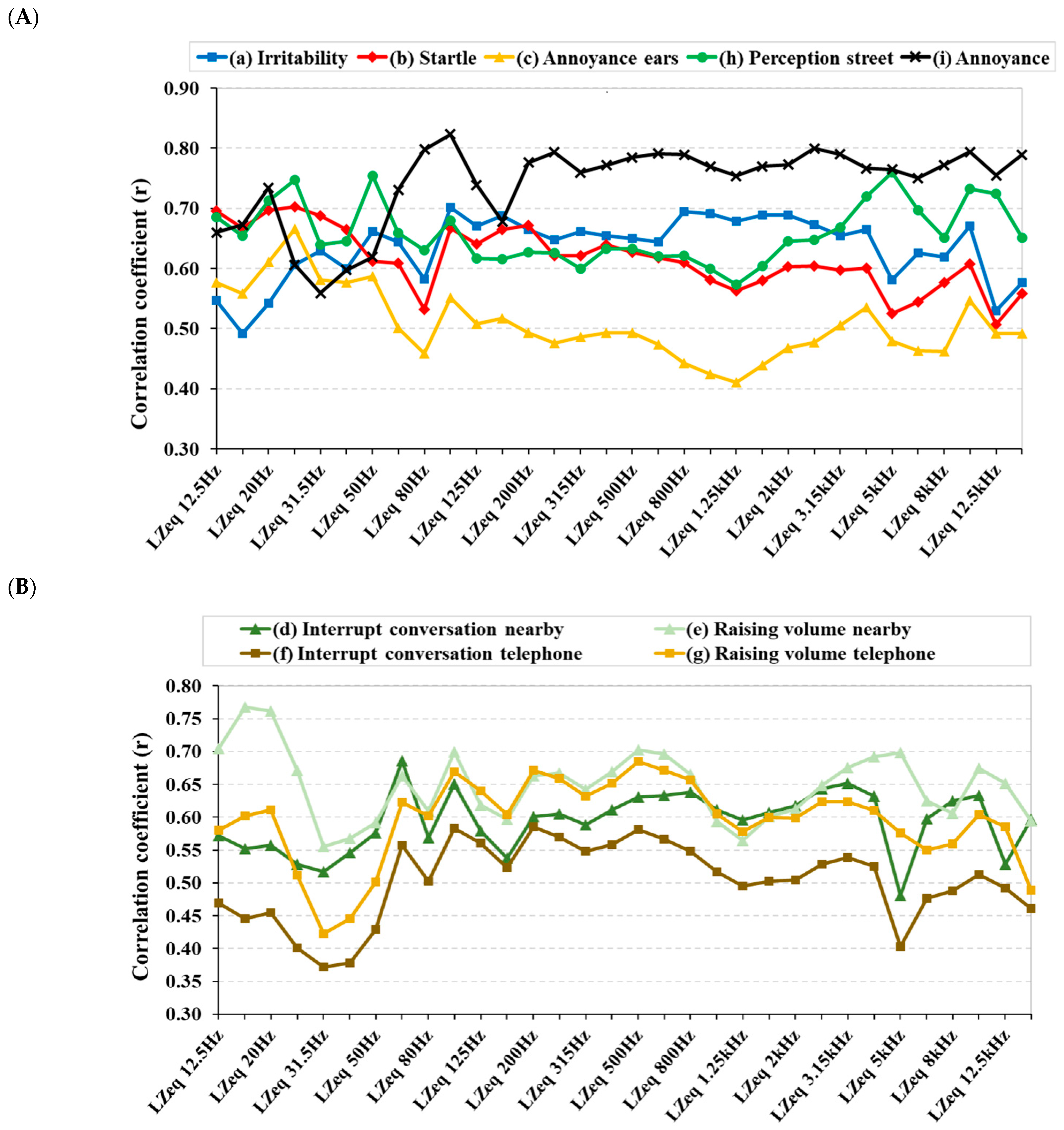
In this section, an analysis is conducted of the explanatory capacity of the acoustic variables that essentially measure sound energy over the whole audible spectrum using different adaptation levels to the response of the human ear (Table 3). According to the way in which these indicators consider the human response in the frequency spectrum, they can be grouped into two blocks. The first are those that have an adaptation independent of sound intensity (equivalent levels), while the second are those in which this adaptation depends on the sound energy. This second group of variables can be further divided into two types: those that consider masking effects (loudness and loudness level), and those that do not (NR, NC, and NCB). From Table 3, it can be seen that all the acoustic variables associated with sound energy over the whole audible spectrum can explain, with significant relations, the occurrence and intensity of all the effects of noise on pedestrians considered in this study.
From a general analysis of Table 3, several points can be noted. It can be seen that the sound variables in the first group (LZeq, LAeq, LCeq, LAIeq, LCIeq) are better able to explain the variability in the effects of noise on pedestrians than those in the second group (loudness, loudness level, NR, NC, NCB), or at least in an equivalent way. From the variables in the first group, for almost all of the subjective variables, LZeq or LCeq are better than or similar to LAeq in terms of explaining the variability in the effects analysed here. Even some of the effects of noise that could be considered in a classic study, such as startle (b), annoyance in the ears (c), and an assessment of the street as noisy (h), the commonly used LAeq indicator is poor in explaining the variability of these three subjective variables and is clearly worse than LZeq. Moreover, the I time weighting, which was used for the LAIeq and LCIeq indicators, had no significant influence on the values of the correlation coefficients for any of the effects studied. In relation to the second group, which relates to different adaptations depending on the sound level, it can firstly be observed that the loudness level or NCB are better than or equivalent to the other three variables (loudness, NR, and NC) in terms of explaining the variability in the effects. Loudness is an indicator that was specifically developed to allow a good relationship with the perception of sound level, and this can be seen to be rather worse than LZeq for the effects of startle (b); annoyance in the ears (c), and in particular (as it is closely related to the objective of this variable), a perception of the street as noisy (h). However, when the values of annoyance (i) were analysed, the results were more as expected. It should also be highlighted that, in general, none of the energy indicators studied here were very effective in explaining the appearance or variability of the effects related to face-to-face or telephone communication, although loudness and loudness level had the highest correlation coefficients in regard to interrupting a phone conversation (f) and raising the volume of their voice on a phone conversation (g), respectively. In this sense, it is worth noting that the difference found for the effect of raising the volume of their voice in a conversation with a nearby person (e) if we compare with the results with the rest of the effects related to verbal communication, (d), (f), and (g), for all the energy indicators except NR and NC. Moreover, for the remaining effects, NR and NC seemed to play a weaker role in explaining the variability of all the subjective variables apart from annoyance (i) and irritability (a). In view of these results, it may be useful to take into account indicators such as NR, NC, and NCB in noise characterisation studies in urban outdoor environments, regardless of whether they are generally used indoors. The outcome for the NCB indicator is of particular interest; it was better than or similar to the others, even when compared to the loudness and loudness level, which are rather more complex indices to obtain, since they take into account in greater detail the way in which humans perceive sounds.
After describing the general aspects listed in Table 3, a detailed analysis was conducted of the implications of these results. Firstly, it is important to point out that the average energy of the sound wave over the full spectrum is a relevant sound characteristic for estimating the occurrence and importance of effects such as irritability (a), startle (b), raising the volume of the conversation in situ (e), the noisy street (h), and annoyance (i), with Pearson correlation coefficients of between 0.70 and 0.81. The highest values for the explanation of variability were obtained for annoyance, and this has a certain uniformity for all the acoustic variables analysed in this section.
In relation to conversations, some differences were found between the variables of raising the volume of the conversation in situ (e) and on the phone (g). When a conversation is held in person, the average energy over the full spectrum is a relevant aspect, and the indicators that do not include weights for low frequencies, such as LZeq or LCeq, seem to explain a higher proportion of the variability than those that do, such as LAeq. On the other hand, if a conversation is held on the phone, the average energy in the full spectrum is less useful, and the medium–high frequency seems to be more important in explaining the variability than the low frequency. When the results for in situ (d) and phone (f) conversation interruption are studied, the in-situ effect is explained to a greater extent. Since all of the acoustic variables have basically the same explanatory power for this effect of noise, this means that high, medium, or low frequencies all seem to have a similar impact.
It is worth noting the result obtained for the loudness indicator, which, in addition to a variable frequency correction depending on the intensity of the sound, takes into account an exponential expression based on the loudness level and the masking effect of some frequencies on others, since it does not seem to be important in the estimation of the relevance of the effects that may be caused by environmental noise. Raising the volume of a telephone conversation (g) is the only effect for which the correlation coefficient for loudness is higher than for the other acoustic indicators of this section. When compared with the values found for LZeq, for example, the loudness results are especially poor for annoyance in the ears (c), with values similar to those obtained for NR and NC. It is important to note that for the variable of annoyance (i), the loudness level and NCB are better indicators than the others with frequency-varying corrections for intensity, including loudness.
As can be observed from Table S1 of the Supplementary Materials, all of the subjective variables were positively correlated with the objective acoustic variables associated with sound energy over the whole audible spectrum, with slope values ranging between 0.13 and 0.35. In general, the highest slope values were found for the relationships between the variables of irritability (a), raising the volume of the conversation (e), interrupting a phone conversation (f), raising the volume of a phone conversation (g), a noisy street (h), and annoyance (i), and the sound indicators LZeq, LCeq, and LCIeq. The results show that a variation of 3 dB in these acoustic variables represents a variation of approximately one point on the 0–10 rating scale for the variables associated with the perception of noise effects.

3.2. Acoustic Variables Associated with Maximum or Minimum Values of Sound Energy

An analysis is presented in this section of the explanatory capacity of acoustic variables that basically measure the maximum and minimum values of the sound energy over the whole audible spectrum and the measurement time, with certain spectral adaptations (A, C) to the response of the human ear, certain temporal considerations with regard to the signal treatment (F, S, I), and also taking into account the signal without temporal treatment (peak). Table 4 shows the correlation coefficients and the levels of significance obtained for the linear relations between the subjective variables and the acoustic variables related to the maximum values of the sound energy.
The first observation that can be made from the group of indicators related to the maximum values of the sound energy, compared to those analysed in the previous section, is that there is a significant loss in their capacity to explain the appearance and intensity of the noise effects analysed. In particular, it is remarkable that the maximum levels have little or no capacity to explain effects such as annoyance in the ears (c) and interruption of a phone conversation (f). This is even unexpected given that effects such as startle (b) or annoyance in the ears (c) could be expected to be explained by the maximum values. Hence, at least for the sound level ranges measured here (see Table 2), the maximum levels are not good estimators of the analysed noise effects.
Despite this, it may be of interest to highlight that an increase in the value of the correlation coefficient is observed for all noise effects when moving from an S weighting to F and I weightings for medium and high frequencies (A weighting). This does not occur for the C-weighted sound indicator columns. This effect may be related to the stronger influence of low frequencies on the value of the indicator when the C weighting is used, and to the fact that a smaller influence from the time weighting is to be expected for longer wavelengths of the sound.
Once the findings related to the maximum values have been analysed, Table 5 shows the correlation coefficients and the levels of significance obtained for the linear relations between the subjective variables and the acoustic variables related to the minimum values of the sound energy. From a first approximation, it can be seen that the indicators of the minimum sound levels analysed here explain a greater proportion of the variability in the noise effects than the indicators of maximum energy. In the case of some of the effects analysed, they are even better in terms of explaining the variability (b, c) or are equivalent (f) to the average energy indicators; this may be an unexpected result, and to the best of the authors’ knowledge, has not been reported previously. The result for effect (c) is particularly remarkable, with a significant increase in the value of the correlation coefficient with respect to that obtained with the average sound energy indicators.
From an overall analysis of this type of indicator in terms of frequency and time weightings, it can be seen that the indicators of minimum values that take into account low frequencies (C weighting) can explain a higher proportion of the variability than those with an A weighting. It should be noted that, so far, the relevance of a low frequency was clear for only three of the effects. For the minimum energy sound indicators, it seems that for all the effects, the C weighting gives better results than the A weighting. These results may indicate that, for some of the effects studied here, both the average and minimum energies may help to explain the appearance or importance of an effect.
Similar behaviour is observed for all in the case of time weightings, although an F weighting achieves the best results. It should be pointed out that for some effects, and mainly those associated with conversation, the I weighting differs more significantly from the F weighting. Finally, it should be noted that, unlike the indicators in the previous section, the least amount of explanation of variability is obtained for annoyance (i). It therefore appears that this effect is most specifically related to the average energy. As is shown in the previous section, this may be the reason why the indicators currently used to measure the effects of environmental noise are mainly based on average energy values. In addition, the results for the A weighting for this effect justify the continued use of this weighting to some extent, even though it is not optimal for other effects, according to the results found in this research.
From Table S1 of the Supplementary Materials, it can be seen that all subjective variables are correlated with the indicators associated with the maximum or minimum values of sound energy, with slope values ranging between 0.07 and 0.29. However, the highest slope values are seen for the indicators of the minimum sound levels. In general, a variation in these minimum energy indicators of between 3.5 and 5 dB corresponds to a variation of approximately one point on the 0–10 rating scale for all subjective variables.

3.3. Acoustic Variables Associated with Sound Energy in Different Parts of the Audible Spectrum

3.3.1. Variables Related to Specific Parts of the Audible Spectrum

This third section shows the results of an analysis of the capacity of the acoustic variables representing the sound energy over the whole period of measurement to explain the variability in the noise effects, by considering the absolute or relative relevance of certain parts of the audible spectrum. Table 6 shows that the acoustic variables Leq20–200Hz, SIL3, SIL, and PSIL are significantly related to the effects of noise under study on pedestrians. For some effects, it could be calculated that they explain around or more than 50% of their variability.
The results for this group of sound indices corroborate the previous findings in Section 3.1, and reinforce the conclusions drawn from them. For the effects of irritability (a), interrupting a conversation (d, and interrupting a phone conversation (f), the low-frequency indicator Leq20–200Hz or the medium- and high-frequency indicators SIL3, SIL, and PSIL give similar results. This also occurs for raising the volume of a conversation (e) with these indicators, although this was not exactly the same as in Section 3.1 for indicators that cover the whole frequency spectrum. In turn, for startle (b), annoyance in the ears (c), and a noisy street (h), it is the low-frequency indicator that explains a higher proportion of its variability, whereas for the effect of raising the volume of a phone conversation (g), the medium- and high-frequency indicators give slightly better results, as in Section 3.1. The medium- and high-frequency indicators again provide the greatest explanation of the variability for annoyance (i).
It can also be seen that indicators that take into account the average energy in some specific parts of the audible spectrum give better results than those that reflect the relative importance of some parts of the spectrum with respect to others. In fact, Leq20–200Hz shows similar results to those obtained with the LZeq, LCeq, and LCIeq indicators, for all the effects analysed here except annoyance (i). In addition, apart from annoyance, the SIL3, SIL, and PSIL indicators have very similar values to the other indicators seen in Section 3.1 and also to each other.
One result that may be striking in principle is that shown by the LCeq-LAeq indicator, with significant negative relationships in the case of the effects of irritability (a) and interrupting conversation (d). These two effects have similarities in terms of the outcomes observed with the different indicators analysed in Table 3 and the results in the first four columns of Table 6. This is interesting because it seems that this indicator, despite giving a low explanation of the variability, may be able to detect a differential effect of the spectrum on the occurrence and importance of these effects, which were not detected by the previous acoustic indicators in Table 3 or the spectral indicators themselves in Table 6. In view of this finding, it seems of interest to perform a study of the sound spectrum in frequency bands to try to analyse in detail what this indicator may be revealing.
Table S1 of the Supplementary Materials shows that all subjective variables are correlated with Leq20–200Hz, SIL3, SIL, and PSIL, with slope values ranging between 0.15 and 0.32. Again, the highest slope values were found for the relations of the variables irritability (a), raising the volume of a conversation (e), interrupting a phone conversation (f), raising the volume of a phone conversation (g), a noisy street (h), and annoyance (i), and the sound indicator Leq20–200Hz. A variation of slightly more than 3 dB in Leq20–200Hz results in a variation of approximately one point on the 0–10 rating scale for these subjective variables.

3.3.2. Analysis in One-Third Octave Frequency Bands

Since the one-third octave frequency bands are those closest to the critical bands of the human ear [38], an analysis was carried out of the relations between the subjective variables associated with the effects of noise and the equivalent sound levels for each of the one-third octave frequency bands. The aim was to study the capacity of the frequency bands to explain the occurrence and importance of the effects considered here. It is necessary to point out that all of the subjective variables related to the effects of noise on pedestrians were significantly correlated with Leq in each of the one-third octave bands with a significance level of at least p ≤ 0.05, and many of these correlations had values of p ≤ 0.01 or p ≤ 0.001. The intensity of these significant correlations can be seen in Figure 4. If the values of the correlation coefficients between variables (a), (b), (c), (h), and (i) with the equivalent unweighted noise levels for each of the one-third octave frequency bands are analysed (Figure 4a), it can be seen that the correlation coefficient for irritability (a) reaches maximum values of around 0.7 in the low-frequency bands between 100 and 160 Hz and in the mid–high frequencies (800–2000 Hz). In this regard, it is worth noting that one of the one-third octave band sections with higher values of the correlation coefficient coincide with the bands where the road traffic noise level reaches the highest values [55]. In the case of startle (b), annoyance in the ears (c), and a noisy street (i), high correlation values were observed with the sound level recorded in the one-third octave frequency band of 25 Hz, with r values of 0.70, 0.67, and 0.75, respectively. In addition, the variable of a noisy street (h) also reached values of approximately 0.75 at 50 Hz and 5 kHz. As is shown in Table 3 and Table 6, the subjective variable of perceived annoyance (i) had the highest correlation coefficient, with values of approximately 0.78 for the one-third octave bands between 200 Hz and 16 kHz and a maximum value of 0.82 at 100 Hz.
From the results of the correlation coefficients between variables (d), (e), (f), and (g) (related to interference within conversations) and the equivalent unweighted noise level for each of the one-third octave frequency bands (Figure 4b), it seems that mid-frequency and low-frequency bands above 50 Hz play a similar role in interruptions to in-person (d) and telephone (f) conversations. However, different results were found when analysing the response to raising the volume of conversations. Low-frequency bands show high relevance in the case of conversations with someone nearby (e), with values for the correlation coefficient of up to 0.77 around the 25 Hz band, whereas mid–high frequency bands are more important in terms of raising the volume in telephone conversations (g), with a maximum r value of 0.68 in the 500 Hz band. This detailed analysis of the one-third octave frequency bands again indicates a possible effect of the noise level measured in the different parts of the audible sound spectrum on the need to raise the voice in conversations, depending on whether they are conducted in the street or by telephone.
In addition, it is of interest to carry out an objective analysis of the possible relation between the structures of the correlation coefficients obtained for the noise spectrum in the one-third octave bands for the different noise effects under study. The aim in this case is to look for similarities in the structure, rather than similarities in the absolute intensity of the explanations. For this purpose, a correlation study was carried out between the values of the correlation coefficients for the different pairs of effects to be considered, such as those in Table 7. The dependent variable was taken as the one that appears in the rows; for example, the results for the Pearson correlation coefficient obtained for the one-third octave frequency bands for irritability (a) are capable of significantly explaining those obtained for the spectrum for the variable of interrupting a conversation with someone nearby (d), with a correlation coefficient of 0.56 and a significance level of p < 0.001.
Several findings can be observed from Table 7. Firstly, it is noted that the frequency band structure that causes the effect of irritability (a) is like the one that causes the effect of interrupting a conversation, regardless of whether it is with someone nearby (d) or on the phone (f). This result, in addition to reinforcing the previous ones, is based on a detailed analysis of their spectra, and indicates a greater degree of similarity between the spectra that cause these three noise effects. In the same way, startle (b) is shown to be closely related to annoyance in the ears (c). Another noteworthy aspect from Table 7 is that the two effects of interrupting a conversation, (d) and (f), seem to have a common cause in terms of the spectrum structure, as well as the effects of having to raise the volume in a face-to-face conversation (e) or on the phone (g). Moreover, when the medium of communication is the telephone, a similar spectral structure of the noise causes both to have to raise the volume (g) or to pause the conversation (f). Something similar takes place in face-to-face conversations, but with a weaker effect. For a perception of the street as noisy (h), the spectral structure of this effect appears to be closely related to that of annoyance in the ears (c) and is also somewhat related to having to raise the volume in a conversation with someone nearby (e). Finally, it is worth noting that annoyance (i) shows similarities in terms of the frequency spectrum with three of the four effects on conversation quality, i.e., (d), (f), and (g).
It may be of interest to note that in some cases, significant linear relationships with a negative sign are obtained, indicating that, to some extent, the structures of the sound spectra that cause some effects are inverse to those that cause others. In this sense, it is important to note, for example, that with a significance value of p ≤ 0.001, the spectral structure related to perceived annoyance (i) is opposite to that related to annoyance in the ears (c), and to that related to startle (b), with p ≤ 0.01. The spectral structure related to perceiving the street as noisy (h) is the opposite of that related to interrupting a conversation on the phone (f) (p ≤ 0.01) or to that related to the effect of irritability (a) (p ≤ 0.05).

4. Conclusions

An experimental study was carried out that involved taking acoustic measurements in the streets of Cáceres (Spain) at the same time as administering pedestrian surveys, in order to study the ability of acoustic variables related to sound energy in urban environments to estimate the occurrence and importance of noise effects. The results obtained in the present study showed that many of the noise effects studied here were significantly correlated with a large proportion of these acoustic variables, reaching values for the correlation coefficient of above 0.8 in some cases.
The findings of the study indicate that the average energy of the sound wave over the full spectrum is an important sound characteristic in terms of explaining the variability of effects such as irritability (a), startle (b), raising the volume of the conversation in situ (e), a noisy street (h), and annoyance (i). For almost all of the effects analysed here, LZeq or LCeq were better than or similar to LAeq in terms of explaining their variability. Moreover, a time I weighting did not have any significant influence on the values of the correlation coefficients for any of the subjective variables. Other indicators that consider different adaptations depending on the sound level, such as loudness, loudness level, NR, NC, and NCB, did not generally provide an improvement, except for interrupting a phone conversation (f), raising the volume of their voice on a phone conversation (g), and annoyance (i).
The indicators based on the minimum sound levels analysed here explained a greater proportion of the variability in the noise effects than the indicators of maximum energy. They were even better for explaining the variability in startle (b) and annoyance in the ears (c), or equivalent for interrupting a phone conversation (f), to all of the average energy indicators. In regard to the minimum energy sound indicators, it seems that the C weighting gives better results than the A weighting for all the noise effects.
Concerning acoustic variables associated with sound energy in different parts of the audible spectrum, it has been found in the present work that Leq20–200Hz, SIL3, SIL, and PSIL were significantly related to the effects of noise under study on pedestrians, with explanations of their variability of around 50% or more. In addition, all subjective variables related to the effects of noise on pedestrians were significantly correlated with Leq in each of the one-third octave bands with a significance level of at least p ≤ 0.05, with different values of the correlation coefficient for each subjective variable depending on the part of the audible spectrum. Similarities in the structure of the spectrum were found between some of these effects.
These findings of this work suggest that urban noise reduction strategies should focus on mitigating low-frequency sounds, which are strongly linked to perceptions of noisiness. Practical measures could include reducing traffic volume, promoting quieter vehicles, and using materials that dampen low-frequency noise. Additionally, using minimum sound level indicators and adopting Z and C weightings for noise assessments can help city managers to better predict and address noise-related health problems other than annoyance, such as irritability or impaired speech communication, thus improving the overall well-being of citizens.
Societies and urban environments can vary in terms of social structures and relationships, traffic patterns, population density, etc. This can influence the acoustic characteristics of environments and also how these characteristics influence the effects of noise on people. This paper has focused on some of the effects of noise and on the energetic characteristics of urban sound environments. The authors are aware of the limitations of their work given the number of surveys (105), although an acceptable statistical power was reached, and the fact that it was carried out in a single city. These results may potentially be valid, at least in urban centres with similar sociological structures, with a similar range of sound level values, and with similar types of noise sources, both traffic and non-traffic related. Thus, the authors encourage the scientific community to carry out studies in other cities with similar approaches and objectives to those proposed in this study. This could perhaps validate and generalise the conclusions of this research. But, it would certainly allow a better understanding of the way in which the different acoustic variables are capable of reflecting the effects of noise on people. In this way, it would advance the development of more effective and perhaps globally applicable urban noise-reduction strategies.

Supplementary Materials

The following supporting information can be downloaded at: https://www.mdpi.com/article/10.3390/app142311212/s1, Questionnaires and Table S1: Slope coefficients of the relations between the subjective and objective variables.

Author Contributions

J.M.B.M.: Conceptualization, Methodology, Software, Validation, Formal analysis, Investigation, Resources, Data Curation, Writing—Original Draft, Writing—Review and Editing, Supervision, Project administration, Funding acquisition. D.M.G.: Methodology, Software, Formal analysis, Investigation, Data Curation, Writing—Original Draft, Writing—Review and Editing, Visualization. R.V.-G.: Methodology, Software, Formal analysis, Investigation, Data Curation, Writing—Review and Editing, Visualization. G.R.-G.: Methodology, Software, Formal analysis, Investigation, Data Curation, Writing—Review and Editing, Visualization. All authors have read and agreed to the published version of the manuscript.

Funding

This project was co-financed by the European Regional Development Fund (ERDF) and Junta de Extremadura (IB18050 and GR21061). This work was also supported by Consejería de Economía, Ciencia y Agenda Digital of Junta de Extremadura through grants for attracting and returning research talent to R&D&I centres belonging to the Extremadura Science, Technology and Innovation System (TA18019), where the University of Extremadura was the beneficiary entity.

Institutional Review Board Statement

The design of the survey was validated by the ethics and bioethics committee of the University of Extremadura in the report with reference 37//2020.

Informed Consent Statement

Surveys of the population were conducted in this study. Following the Declaration of Helsinki, each participant filled out a declaration of informed consent.

Data Availability Statement

The original contributions presented in the study are included in the article/supplementary material, further inquiries can be directed to the corresponding author.

Acknowledgments

The authors would like to acknowledge the contribution of Pedro Atanasio, Ana Bejarano, and Manuel Parejo for their contribution during the measurement and survey process.

Conflicts of Interest

The authors declare no conflicts of interest.

References

  1. Hahad, O.; Jimenez, M.T.B.; Kuntic, M.; Frenis, K.; Steven, S.; Daiber, A.; Münzel, T. Cerebral consequences of environmental noise exposure. Environ. Int. 2022, 165, 107306. [Google Scholar] [CrossRef]
  2. Tangermann, L.; Vienneau, D.; Hattendorf, J.; Saucy, A.; Künzli, N.; Schäffer, B.; Wunderli, J.M.; Röösli, M. The association of road traffic noise with problem behaviour in adolescents: A cohort study. Environ. Res. 2022, 207, 112645. [Google Scholar] [CrossRef]
  3. Begou, P.; Kassomenos, P.; Kelessis, A. Effects of road traffic noise on the prevalence of cardiovascular diseases: The case of Thessaloniki, Greece. Sci. Total Environ. 2020, 703, 134477. [Google Scholar] [CrossRef] [PubMed]
  4. Min, J.; Min, K. Cumulative exposure to nighttime environmental noise and the incidence of peptic ulcer. Environ. Int. 2018, 121, 1172–1178. [Google Scholar] [CrossRef] [PubMed]
  5. Fiorini, C.V. Railway noise in urban areas: Assessment and prediction on infrastructure improvement combined with settlement development and regeneration in central Italy. Appl. Acoust. 2022, 185, 108413. [Google Scholar] [CrossRef]
  6. Barrigón Morillas, J.M.; Rey Gozalo, G.; Montes Gonzalez, D.; Sánchez-Fernández, M.; Bachiller León, A. A comprehensive experimental study of the influence of temperature on urban road traffic noise under real-world conditions. Environ. Pollut. 2022, 309, 119761. [Google Scholar] [CrossRef] [PubMed]
  7. Wing, S.E.; Larson, T.V.; Hudda, N.; Boonyarattaphan, S.; Rosario, I.D.; Fruin, S.; Ritz, B. Aircraft noise and vehicle traffic-related air pollution interact to affect preterm birth risk in Los Angeles, California. Sci. Total Environ. 2022, 829, 154678. [Google Scholar] [CrossRef] [PubMed]
  8. EEA. Outlook to 2030—Can the Number of People Affected by Transport Noise Be Cut by 30%? European Environment Agency; Publications Office of the European Union: Luxembourg, 2022. [Google Scholar]
  9. COM/2021/400. Pathway to a Healthy Planet for All EU Action Plan: Towards Zero Pollution for Air, Water and Soil; European Commission: Brussels, Belgium, 2021. [Google Scholar]
  10. Wosniacki, G.G.; Zannin, P.H.T. Framework to manage railway noise exposure in Brazil based on field measurements and strategic noise mapping at the local level. Sci. Total Environ. 2021, 757, 143721. [Google Scholar] [CrossRef]
  11. Rey-Gozalo, G.; Barrigón Morillas, J.M.; Montes González, D. Analysis and Management of Current Road Traffic Noise. Curr. Pollut. Rep. 2022, 8, 315–327. [Google Scholar] [CrossRef]
  12. Khomenko, S.; Cirach, M.; Barrera-Gómez, J.; Pereira-Barboza, E.; Iungman, T.; Mueller, N.; Foraster, M.; Tonne, C.; Thondoo, M.; Jephcote, C.; et al. Impact of road traffic noise on annoyance and preventable mortality in European cities: A health impact assessment. Environ. Int. 2022, 162, 107160. [Google Scholar] [CrossRef]
  13. Faulkner, J.-P.; Murphy, E. Road traffic noise modelling and population exposure estimation using CNOSSOS-EU: Insights from Ireland. Appl. Acoust. 2022, 192, 108692. [Google Scholar] [CrossRef]
  14. Rey Gozalo, G.; Gómez Escobar, V.; Barrigón Morillas, J.M.; Montes González, D.; Atanasio Moraga, P. Statistical attribution of errors in urban noise modeling. Appl. Acoust. 2019, 153, 20–29. [Google Scholar] [CrossRef]
  15. Prezelj, J.; Murovec, J. Traffic noise modelling and measurement: Inter-laboratory comparison. Appl. Acoust. 2017, 127, 160–168. [Google Scholar] [CrossRef]
  16. Can, A.; L’Hostis, A.; Aumond, P.; Botteldooren, D.; Coelho, M.C.; Guarnaccia, C.; Kang, J. The future of urban sound environments: Impacting mobility trends and insights for noise assessment and mitigation. Appl. Acoust. 2020, 170, 107518. [Google Scholar] [CrossRef]
  17. Paschalidou, A.K.; Kassomenos, P.; Chonianaki, F. Strategic Noise Maps and Action Plans for the reduction of population exposure in a Mediterranean port city. Sci. Total Environ. 2019, 654, 144–153. [Google Scholar] [CrossRef]
  18. Licitra, G.; Ascari, E.; Fredianelli, L. Prioritizing Process in Action Plans: A Review of Approaches. Curr. Pollut. Rep. 2017, 3, 151–161. [Google Scholar] [CrossRef]
  19. Barrigón Morillas, J.M.; Rey Gozalo, G.; Montes González, D.; Vílchez-Gómez, R.; Gómez-Escobar, V. Variability of traffic noise pollution levels as a function of city size variables. Environ. Res. 2021, 199, 111303. [Google Scholar] [CrossRef] [PubMed]
  20. Han, X.; Huang, X.; Liang, H.; Ma, S.; Gong, J. Analysis of the relationships between environmental noise and urban morphology. Environ. Pollut. 2018, 233, 755–763. [Google Scholar] [CrossRef] [PubMed]
  21. Ariza-Villaverde, A.B.; Jiménez-Hornero, F.J.; Ravé, E.G.D. Influence of urban morphology on total noise pollution: Multifractal description. Sci. Total Environ. 2014, 472, 1–8. [Google Scholar] [CrossRef]
  22. Wang, P.; Zhou, B.; Han, L.; Mei, R. The motivation and factors influencing visits to small urban parks in Shanghai, China. Urban For. Urban Green. 2021, 60, 127086. [Google Scholar] [CrossRef]
  23. Misiune, I.; Julian, J.P.; Veteikis, D. Pull and push factors for use of urban green spaces and priorities for their ecosystem services: Case study of Vilnius, Lithuania. Urban For. Urban Green. 2021, 58, 126899. [Google Scholar] [CrossRef]
  24. Rey Gozalo, G.; Barrigon Morillas, J.M.; Montes Gonzalez, D. Perceptions and use of urban green spaces on the basis of size. Urban For. Urban Green. 2019, 46, 126470. [Google Scholar] [CrossRef]
  25. Gidlöf-Gunnarsson, A.; Öhrström, E. Noise and well-being in urban residential environments: The potential role of perceived availability to nearby green areas. Landsc. Urban Plan. 2007, 83, 115–126. [Google Scholar] [CrossRef]
  26. Lionello, M.; Aletta, F.; Kang, J. A systematic review of prediction models for the experience of urban soundscapes. Appl. Acoust. 2020, 170, 107479. [Google Scholar] [CrossRef]
  27. Maristany, A.; López, M.R.; Rivera, C.A. Soundscape quality analysis by fuzzy logic: A field study in Cordoba, Argentina. Appl. Acoust. 2016, 111, 106–115. [Google Scholar] [CrossRef]
  28. Ricciardi, P.; Delaitre, P.; Lavandier, C.; Torchia, F.; Aumond, P. Sound quality indicators for urban places in Paris cross-validated by Milan data. J. Acoust. Soc. Am. 2015, 138, 2337–2348. [Google Scholar] [CrossRef] [PubMed]
  29. Cleary-Gaffney, M.; Espey, B.; Coogan, A.N. Association of perceptions of artificial light-at-night, light-emitting device usage and environmental noise appraisal with psychological distress, sleep quality and chronotype: A cross sectional study. Heliyon 2022, 8, e11284. [Google Scholar] [CrossRef]
  30. Li, W.; Zhai, J.; Zhu, M. Characteristics and perception evaluation of the soundscapes of public spaces on both sides of the elevated road: A case study in Suzhou, China. Sustain. Cities Soc. 2022, 84, 103996. [Google Scholar] [CrossRef]
  31. Zhang, L.; Ma, H. Investigation of Chinese residents’ community response to high-speed railway noise. Appl. Acoust. 2021, 172, 107615. [Google Scholar] [CrossRef]
  32. Morihara, T.; Sato, T.; Yano, T. Re-analysis of socio-acoustic survey data in Tomakomai: Seasonal effects of a tree belt on road traffic noise annoyance. Appl. Acoust. 2022, 196, 108861. [Google Scholar] [CrossRef]
  33. Okokon, E.O.; Turunen, A.W.; Ung-Lanki, S.; Vartiainen, A.-K.; Tiittanen, P.; Lanki, T. Road-traffic noise: Annoyance, risk perception, and noise sensitivity in the finnish adult population. Int. J. Environ. Res. Public. Health 2015, 12, 5712–5734. [Google Scholar] [CrossRef] [PubMed]
  34. Montes González, D.; Barrigón Morillas, J.M.; Rey-Gozalo, G. Effects of noise on pedestrians in urban environments where road traffic is the main source of sound. Sci. Total Environ. 2023, 857, 159406. [Google Scholar] [CrossRef] [PubMed]
  35. Ma, K.W.; Mak, C.M.; Wong, H.M. Effects of environmental sound quality on soundscape preference in a public urban space. Appl. Acoust. 2021, 171, 107570. [Google Scholar] [CrossRef]
  36. Paszkowski, W.; Kotus, J.; Poremski, T.; Kostek, B. Evaluation of sound quality features on environmental noise effects—A case study applied to road traffic noise. Metrol. Meas. Syst. 2018, 25, 517–531. [Google Scholar] [CrossRef]
  37. Rey-Gozalo, G.; Trujillo Carmona, J.; Barrigón Morillas, J.M.; Vílchez-Gómez, R.; Gómez Escobar, V. Relationship between objective acoustic indices and subjective assessments for the quality of soundscapes. Appl. Acoust. 2015, 97, 1–10. [Google Scholar] [CrossRef]
  38. Fastl, H.; Zwicker, E. Psychoacoustics: Facts and Models, Psychoacoustics: Facts and Models; Springer: Berlin/Heidelberg, Germany, 2007. [Google Scholar] [CrossRef]
  39. Barrigón Morillas, J.M.; Montes Gonzalez, D.; Gómez Escobar, V.; Rey Gozalo, G.; Vílchez-Gómez, R. A proposal for producing calculated noise mapping defining the sound power levels of roads by street stratification. Environ. Pollut. 2021, 270, 116080. [Google Scholar] [CrossRef]
  40. INE (Instituto Nacional de Estadística), 2021. Censo de Población y Viviendas. Instituto Nacional de Estadística, Madrid. Available online: https://www.ine.es/Censo2021/Wizard.do?WIZARD=1&reqCode=pasoSeleccionColectivo (accessed on 20 October 2024).
  41. Deutskens, E.; de Ruyter, K.; Wetzels, M.; Oosterveld, P. Response Rate and Response Quality of Internet-Based Surveys: An Experimental Study. Mark. Lett. 2004, 15, 21–36. [Google Scholar] [CrossRef]
  42. Wu, M.-J.; Zhao, K.; Fils-Aime, F. Response rates of online surveys in published research: A meta-analysis. Comput. Hum. Behav. Rep. 2022, 7, 100206. [Google Scholar] [CrossRef]
  43. Díaz de Rada Igúzquiza, V.; Palacios Gómez, J.L. Comparación de las tasas de respuesta en el uso combinado de modalidades de encuesta. Rev. Esp. Invest. Sociol. 2024, 141, 159–170. [Google Scholar] [CrossRef]
  44. Fritz, M.S.; MacKinnon, D.P. Required sample size to detect the mediated effect. Psychol. Sci. 2007, 18, 233–239. [Google Scholar] [CrossRef]
  45. Cohen, J. Statistical Power Analysis for the Behavioral Sciences, 2nd ed.; Lawrence Erlbaum Associates: Mahwah, NJ, USA, 1988. [Google Scholar] [CrossRef]
  46. National Institute of Statistics. 2021. Available online: https://www.ine.es/ss/Satellite?L=es_ES&c=INESeccion_C&p=1254735110672&pagename=ProductosYServicios%2FPYSLayout&param1=PYSDetalleFichaSeccionUA&param3=1259944561392&_charset_=UTF-8&cid=1259944638308 (accessed on 20 October 2024).
  47. Rodríguez del Águila, M.M.; González-Ramírez, A.R. Sample size calculation. Allergol. Immunopathol. 2014, 42, 485–492. [Google Scholar] [CrossRef] [PubMed]
  48. Paiva, K.M.; Cardoso, M.R.A.; Zannin, P.H.T. Exposure to road traffic noise: Annoyance, perception and associated factors among Brazil’s adult population. Sci. Total Environ. 2019, 650, 978–986. [Google Scholar] [CrossRef]
  49. Tao, Y.; Chai, Y.; Kou, L.; Kwan, M.-P. Understanding noise exposure, noise annoyance, and psychological stress: Incorporating individual mobility and the temporality of the exposure-effect relationship. Appl. Geogr. 2020, 125, 102283. [Google Scholar] [CrossRef]
  50. Montes González, D.; Barrigón Morillas, J.M.; Rey Gozalo, G.; Godinho, L. Evaluation of exposure to road traffic noise: Effects of microphone height and urban configuration. Environ. Res. 2020, 191, 110055. [Google Scholar] [CrossRef]
  51. Barrigón Morillas, J.M.; Montes González, D.; Rey Gozalo, G. A review of the measurement procedure of the ISO 1996 standard. Relationship with the European Noise Directive. Sci. Total Environ. 2016, 565, 595–606. [Google Scholar] [CrossRef] [PubMed]
  52. Zagubień, A.; Wolniewicz, K. Impact of measuring microphone location on the result of environmental noise assessment. Appl. Acoust. 2021, 172, 107662. [Google Scholar] [CrossRef]
  53. Montes González, D.; Barrigón Morillas, J.M.; Rey Gozalo, G.; Atanasio Moraga, P. Microphone position and noise exposure assessment of building façades. Appl. Acoust. 2020, 160, 107157. [Google Scholar] [CrossRef]
  54. Montes González, D.; Barrigón Morillas, J.M.; Rey Gozalo, G.; Godinho, L. Effect of parking lanes on assessing the impact of road traffic noise on building façades. Environ. Res. 2020, 184, 109299. [Google Scholar] [CrossRef]
  55. UNE-EN 1793-3:1998; Road Traffic Noise Reducing Devices—Test Method for Determining the Acoustic Performance—Part 3: Normalized Traffic Noise Spectrum. Spanish Association for Standardization: Madrid, Spain, 1998.
Figure 1. Survey points in Cáceres (from Google Earth).
Applsci 14 11212 g001
Figure 2. A box plot of the answers for the subjective variables (a)–(i).
Applsci 14 11212 g002
Figure 3. One-third octave band noise profile of the measurements at the different points considered.
Applsci 14 11212 g003
Figure 4. Correlation coefficients between subjective variables and the equivalent unweighted noise level for each of the 1/3 octave frequency bands: (A) variables (a), (b), (c), (h) and (i); (B) variables (d), (e), (f), and (g).
Applsci 14 11212 g004
Table 1. Sociodemographic characteristics of the sample.
VariableSample (%)Cáceres (%) [40]
Age
18–25 years19.06.7
26–35 years11.410.7
36–45 years21.015.1
46–55 years20.016.8
56–65 years13.314.8
>66 years15.218.0
Sex
Male43.848.1
Female56.251.9
Education
Missing-8.2
Primary or secondary school23.833.9
High school24.817.9
Degree51.433.8
Work activity
Worker59.041.7
Unemployed6.79.0
Retired16.213.1
Homemaker6.711.9
Student11.422.0
Table 2. Subjective and objective variables registered in the city of Cáceres, together with a brief description of their meaning and the range of values for each of them.
VariablesMeaningValue Range
(a)Irritability0–10
(b)Startle0–10
(c)Annoyance in the ears0–10
(d)Interruption of a conversation with someone nearby0–10
(e)Raising the volume of their voice to speak with someone nearby0–10
(f)Interruption of a phone conversation0–10
(g)Raising the volume of their voice during a phone conversation0–10
(h)Noisiness of the street0–10
(i)Annoyance 0–10
Acoustic objective variables (measurements)Energy (full audible spectrum)LZeqUnweighted equivalent sound level60–81 dB
LAeqA-weighted equivalent sound level48–73 dB
LCeqC-weighted equivalent sound level58–79 dB
LAIeqA,I-weighted equivalent sound level52–75 dB
LCIeqC,I-weighted equivalent sound level63–81 dB
LoudnessSubjective judgement of the intensity of a sound7–30 sones
Loudness levelLoudness level = 10 × log2(Loudness) + 4068–89 phones
NRHighest noise ratio curve touched by the measured spectrum45–71
NCHighest noise criteria curve touched by the measured spectrum43–70
NCBHighest balanced noise criteria curve touched by the measured spectrum42–65
Energy (maximum or minimum)LASmaxA,S-weighted maximum sound level68–87 dB
LAFmaxA,F-weighted maximum sound level70–89 dB
LAImaxA,I-weighted maximum sound level70–91 dB
LCSmaxC,S-weighted maximum sound level77–96 dB
LCFmaxC,F-weighted maximum sound level80–99 dB
LCImaxC,I-weighted maximum sound level81–100 dB
LCpeakC-weighted peak sound level90–111 dB
LASminA,S-weighted minimum sound level35–55 dB
LAFminA,F-weighted minimum sound level33–54 dB
LAIminA,I-weighted minimum sound level35–55 dB
LCSminC,S-weighted minimum sound level48–65 dB
LCFminC,F-weighted minimum sound level46–62 dB
LCIminC,I-weighted minimum sound level49–66 dB
Energy (parts of audible spectrum)Leq20–200HzEquivalent sound level in the range 20–200 Hz59–81 dB
SIL3Speech interference level (average Leq of 1000, 2000 and 4000 Hz octave bands)41–65 dB
SILSpeech interference level (average Leq of 500, 1000, 2000 and 4000 Hz octave bands)42–65 dB
PSILPreferred speech interference level (average Leq of 500, 1000 and 2000 Hz octave bands)43–68 dB
LCeq − LAeqDifference between LCeq and LAeq1–4 dB
Table 3. Correlation coefficients between subjective variables and acoustic variables associated with sound energy over the whole audible spectrum.
LZeqLAeqLCeqLAIeqLCIeqLoudnessLoudness LevelNRNCNCB
(a)0.70 ***0.69 ***0.71 ***0.67 ***0.69 ***0.67 ***0.69 ***0.69 ***0.69 ***0.69 ***
(b)0.70 ***0.61 ***0.68 ***0.61 ***0.69 ***0.59 ***0.62 ***0.59 ***0.59 ***0.62 ***
(c)0.60 ***0.46 *0.58 **0.46 *0.57 **0.45 *0.50 **0.43 *0.43 *0.49 **
(d)0.64 ***0.63 ***0.64 ***0.62 ***0.64 ***0.61 ***0.63 ***0.62 ***0.63 ***0.62 ***
(e)0.71 ***0.65 ***0.68 ***0.67 ***0.69 ***0.66 ***0.67 ***0.61 ***0.63 ***0.66 ***
(f)0.53 **0.54 **0.53 **0.53 **0.51 **0.53 **0.55 **0.52 **0.54 **0.53 **
(g)0.62 ***0.64 ***0.62 ***0.65 ***0.62 ***0.66 ***0.64 ***0.61 ***0.63 ***0.64 ***
(h)0.75 ***0.63 ***0.73 ***0.64 ***0.72 ***0.63 ***0.67 ***0.61 ***0.61 ***0.66 ***
(i)0.76 ***0.79 ***0.76 ***0.81 ***0.76 ***0.79 ***0.80 ***0.77 ***0.79 ***0.81 ***
* Significant at p ≤ 0.05. ** Significant at p ≤ 0.01. *** Significant at p ≤ 0.001.
Table 4. Correlation coefficients between subjective variables and acoustic variables related to the maximum values of the sound energy.
LASmaxLAFmaxLAImaxLCSmaxLCFmaxLCImaxLCpeak
(a)0.53 **0.57 **0.58 ***0.46 *0.43 *0.45 *0.53 **
(b)0.34 n.s.0.41 *0.46 *0.37 *0.39 *0.46 *0.50 **
(c)0.19 n.s.0.26 n.s.0.30 n.s.0.32 n.s.0.31 n.s.0.35 n.s.0.36 n.s.
(d)0.42 *0.44 *0.45 *0.36 n.s.0.36 n.s.0.34 n.s.0.22 n.s.
(e)0.41 *0.50 **0.53 **0.39 *0.40 *0.39 *0.30 n.s.
(f)0.27 n.s.0.28 n.s.0.31 n.s.0.31 n.s.0.30 n.s.0.27 n.s.0.14 n.s.
(g)0.35 n.s.0.42 *0.45 *0.37 *0.38 *0.36 n.s.0.26 n.s.
(h)0.37 *0.47 *0.51 **0.49 **0.49 **0.48 **0.46 *
(i)0.61 ***0.67 ***0.70 ***0.53 **0.55 **0.55 **0.50 **
n.s. Non-significant correlation (p > 0.05). * Significant at p ≤ 0.05. ** Significant at p ≤ 0.01. *** Significant at p ≤ 0.001.
Table 5. Correlation coefficients between subjective variables and acoustic variables related to the minimum values of the sound energy.
LASminLAFminLAIminLCSminLCFminLCImin
(a)0.56 **0.59 ***0.56 **0.66 ***0.66 ***0.66 ***
(b)0.66 ***0.69 ***0.66 ***0.71 ***0.72 ***0.70 ***
(c)0.66 ***0.69 ***0.66 ***0.69 ***0.70 ***0.66 ***
(d)0.55 **0.57 **0.55 **0.60 ***0.61 ***0.60 ***
(e)0.56 **0.54 **0.56 **0.57 **0.58 **0.55 **
(f)0.52 **0.54 **0.52 **0.52 **0.55 **0.51 **
(g)0.53 **0.53 **0.52 **0.52 **0.54 **0.49 **
(h)0.57 **0.60 ***0.58 ***0.66 ***0.66 ***0.65 ***
(i)0.46 *0.45 *0.46 *0.49 **0.50 **0.49 **
* Significant at p ≤ 0.05. ** Significant at p ≤ 0.01. *** Significant at p ≤ 0.001.
Table 6. Correlation coefficients between subjective variables and acoustic variables associated with sound energy in different parts of the audible spectrum.
Leq20−200HzSIL3SILPSILLCeq-LAeq
(a)0.69 ***0.69 ***0.68 ***0.68 ***−0.42 *
(b)0.69 ***0.60 ***0.61 ***0.61 ***−0.25 n.s.
(c)0.61 ***0.47 *0.48 **0.46 *−0.26 n.s.
(d)0.62 ***0.62 ***0.63 ***0.63 ***−0.38 *
(e)0.67 ***0.65 ***0.67 ***0.65 ***−0.11 n.s.
(f)0.50 **0.52 **0.54 **0.54 **0.35 n.s.
(g)0.58 ***0.63 ***0.64 ***0.64 ***−0.25 n.s.
(h)0.75 ***0.66 ***0.66 ***0.63 ***−0.27 n.s.
(i)0.72 ***0.80 ***0.80 ***0.79 ***−0.36 n.s.
n.s. Non-significant correlation (p > 0.05). * Significant at p ≤ 0.05. ** Significant at p ≤ 0.01. *** Significant at p ≤ 0.001.
Table 7. Correlation coefficients between the values of the correlation coefficients of variables (a)–(i) in Figure 4.
(b)(c)(d)(e)(f)(g)(h)(i)
(a)−0.01 n.s.−0.38 *0.56 ***−0.38 *0.53 **0.32 n.s.−0.39 *0.31 n.s.
(b) 0.70 ***−0.08 n.s.0.29 n.s.−0.07 n.s.−0.02 n.s.−0.03 n.s.−0.52 **
(c) −0.38 *0.31 n.s.−0.50 **−0.41 *0.60 ***−0.68 ***
(d) 0.11n.s.0.73 ***0.54 **−0.30 n.s.0.60 ***
(e) 0.24 n.s.0.55 **0.37 *0.25 n.s.
(f) 0.90 ***−0.45 **0.74 ***
(g) −0.29 n.s.0.74 ***
(h) −0.23 n.s.
n.s. Non-significant correlation (p > 0.05). * Significant at p ≤ 0.05. ** Significant at p ≤ 0.01. *** Significant at p ≤ 0.001.
Disclaimer/Publisher’s Note: The statements, opinions and data contained in all publications are solely those of the individual author(s) and contributor(s) and not of MDPI and/or the editor(s). MDPI and/or the editor(s) disclaim responsibility for any injury to people or property resulting from any ideas, methods, instructions or products referred to in the content.

