Abstract
Brain–computer interfaces (BCIs) are essential in advancing medical diagnosis and treatment by providing non-invasive tools to assess neurological states. Among these, motor imagery (MI), in which patients mentally simulate motor tasks without physical movement, has proven to be an effective paradigm for diagnosing and monitoring neurological conditions. Electroencephalography (EEG) is widely used for MI data collection due to its high temporal resolution, cost-effectiveness, and portability. However, EEG signals can be noisy from a number of sources, including physiological artifacts and electromagnetic interference. They can also vary from person to person, which makes it harder to extract features and understand the signals. Additionally, this variability, influenced by genetic and cognitive factors, presents challenges for developing subject-independent solutions. To address these limitations, this paper presents a Multimodal and Explainable Deep Learning (MEDL) approach for MI-EEG classification and physiological interpretability. Our approach involves the following: (i) evaluating different deep learning (DL) models for subject-dependent MI-EEG discrimination; (ii) employing class activation mapping (CAM) to visualize relevant MI-EEG features; and (iii) utilizing a questionnaire–MI performance canonical correlation analysis (QMIP-CCA) to provide multidomain interpretability. On the GIGAScience MI dataset, experiments show that shallow neural networks are good at classifying MI-EEG data, while the CAM-based method finds spatio-frequency patterns. Moreover, the QMIP-CCA framework successfully correlates physiological data with MI-EEG performance, offering an enhanced, interpretable solution for BCIs.
1. Introduction
The 2021 UNESCO Engineering for Sustainable Development report points out the role the profession has on the 2030 Agenda. The third goal, “ensure healthy lives and promote well-being for all at all ages”, highlights the advancements in improving medical diagnosis and care through low-cost tools [1]. The most affordable tool in neuroscience is electroencephalography (EEG), which is also the most studied, thanks to its high temporal resolution and portability. EEG captures subjects’ neural bioelectric activity generated via neuron activation through electrodes placed on the scalp [2]. Techniques like event-related potentials (ERPs) extract representative time-frequency information within the time-series data to understand the neurological activity of a subject or a group [3]. Also, brain–computer interfaces (BCIs) profit from those patterns for controlling external devices, such as prostheses [4]. To learn brain patterns, a BCI paradigm presents stimuli and asks the subject to perform tasks. For instance, the motor imagery (MI) paradigm, which consists of the mental rehearsal of motor tasks without physical movement, has been used to support the diagnosis, treatment, and follow-up of brain diseases [5].
However, EEG is far from the panacea for all neuroimaging needs. Due to its non-invasive nature, superficial EEG sacrifices spatial resolution and becomes highly susceptible to electromagnetic artifacts (e.g., electrical devices) and physiological noise (e.g., eye movement and muscle activity), yielding less useful features [6,7]. Moreover, the volume conduction effect introduces noise or cross-talk between electrodes, hampering the source localization of brain activity and the interpretation of EEG data [8]. Lastly, both between- and within-subject variability challenge the development of a universal MI-EEG algorithm. Differences in genetic, cognitive, and neurodevelopmental factors cause the same task or stimuli to evoke distinct brain patterns across individuals, complicating the creation of subject-independent solutions [9,10]. Additionally, as users become more familiar with the BCI device or task over time, their performance and initial brain patterns evolve, demanding personalized calibration sessions [11].
Traditional MI-EEG algorithms attempt to extract features by analyzing the signal’s power levels. The baseline common spatial patterns (CSPs) exploit the power distribution over the scalp to find spatial patterns discriminating between two tasks [12]. Variations of CSPs include the following: L1-CSP, which regularizes the patterns using the L1-norm; sparse filter-band CSP (SFBCSP), which automatically selects useful spectral bands from a precomputed set [13]; and multi-kernel Stein spatial patterns (MKSSPs), which extract nonlinear patterns in a low-dimensional Riemannian manifold [14]. However, a low signal-to-noise ratio makes CSPs and their variants extract features from artifacts, rather than an actual EEG [15].
Conversely, machine learning algorithms exploit their ability to automatically learn features from a given training dataset to minimize the prediction error as much as possible [16]. Deep learning (DL) methods extract nonlinear patterns, dealing with EEG noise and volume conduction effect [17]. Convolutional neural networks (CNNs), a DL model, are the most successful EEG feature extraction architectures because they look for space and time patterns [18]. Examples of CNNs for MI-EEG classification are EEGNet, ShallowConvNet, and DeepConvNet, which, like SFBCSP, also extract spatial patterns from certain frequency bands [19]. Unlike SFBCSP, the above architectures unravel nonlinear, deeper, and more complex patterns [20]. Other DL models for EEG applications include autoencoders that embed EEG signals into a generative noise-reduced feature space [21], recurrent neural networks (RNNs) that exploit the sequential nature of EEG features [22], and, more recently, transformers that use their long-term memory to capture both global and local patterns [23].
However, there are two main concerns about the medical applications of the above DL models. Firstly, they become “black boxes”, lacking interpretable information to understand each subject’s neurological abilities [24]. Secondly, they ignore the closed link between neurological, physiological, and personal behaviors [25]. Analyzing how these factors influence the model provides users and scientists with valuable information to improve the results beforehand. Thus, multimodal and multidomain strategies can couple information from patients’ moods and habits to understand their neurophysiological responses and exploit this additional information to improve model performance and interpretability.
This work proposes multimodal and explainable deep learning (MEDL) as an approach to MI-EEG discrimination and physiological interpretability. Specifically, our proposal is threefold: (i) Different DL models are tested for subject-dependent MI-EEG discrimination. (ii) A CAM-based approach is used to quantify and visualize relevant MI-EEG features. (iii) A questionnaire–MI performance canonical correlation analysis (QMIP-CCA) strategy is introduced as a multidomain explainability stage for physiological and MI-EEG discrimination non-linear feature matching. Experiments are carried out with the GIGAScience MI dataset due to its relatively large number of subjects and the additional questionnaire that it offers for physiological subject information [26]. The results obtained demonstrate that shallow networks achieve acceptable MI discrimination results. In addition, our CAM-based method allows us to code MI group patterns and measure EEG features of the sensorimotor cortex in people who are getting better at MI. Finally, our QMIP-CCA allows for quantifying and visualizing relevant physiological questions from tabular data and matching them to MI-EEG performance measures.
2. Related Work
Since Koles et al.’s work in 1990, CSP has been the go-to tool for feature extraction from EEG data [27]. CSP provides spatial filters that maximize the variance ratio of two multivariate signals, enabling the discrimination of two classes for classification purposes. Unfortunately, since the technique depends on the signals’ variance, it becomes sensitive to noise and struggles with small datasets [28]. In turn, variants of CSP have sprung up to enhance the original algorithm. L1CSP redefines the base objective in terms of the L1-norm instead of the usual L2-norm to reduce artifacts’ influence on the signal [29]. In contrast, FBCSP adds a bandpass filtering stage for multiple, manually selected frequency bands before the usual spatial filtering. After that, it uses a mutual information algorithm to select discriminant features [30]. Lastly, SFBCSP selects the bandpass filters semi-automatically, rather than manually like FBCSP, by integrating a sparse regression model to learn the optimal features from each input filter band [31]. However, these models remain power-reliant and, in the case of FBCSP and SFBCSP, require some form of manual input. Once features have been extracted, classification can be performed through various methods. One such technique is support vector machines (SVMs). SVMs work by finding the optimal hyperplane for separating classes [32]. However, SVMs fail to classify data when features are too similar between classes [33].
Thanks to their ability to recognize and extract non-linear features from raw EEG data [34], DL models solve many of these traditional algorithms’ shortcomings. CNNs are a family of DL strategies that scan the input signal for representative patterns, starting from simple structures until reaching a more complex combination of these initial features. These algorithms are commonly used for image processing, but by tuning the size and number of filters, it is possible to extract information from the temporal, spatial, and frequency domains, e.g., for MI-EEG classification. Also, unlike CSP, these models automatically fine-tune the best filters for the given task through gradient descent [35]. Some relevant examples of CNNs for MI-EEG include EEGNet, KREEGNet, ShallowConvNet, DeepConvNet, TCFusionnet, and KCS-FCNet.
In particular, EEGNet obtains different features from EEG data in three steps: temporal convolution, depthwise convolution (to find patterns in time and space), and separable convolution (to combine the data from the first two steps) [36]. Variations of this original architecture have since emerged. TCFusionNet, for example, integrates the EEGNet architecture with residual blocks composed of dilated convolutions, which add these residual features to the ones from the separable convolution to increase the size of the receptive field while avoiding the exploding/vanishing gradient problem of deeper models [37]. ShallowConvNet works similarly to EEGNet but skips the separable convolution stage and uses regular convolution for spatial filtering. This reduces the number of parameters requiring training, leading to faster training and better interpretability, but at the cost of some performance. DeepConvNet, on the other hand, goes much further by adding a series of 2D convolutions that get bigger and bigger in order to pull information from the earlier stages and find complex structures [19]. Regarding deep kernel learning (DKL) methods, KREEGNet computes the functional connectivities from the temporal convolution through Gaussian similarity, alongside a delta kernel for label outputs, all to use central kernel alignment (CKA) as a regularizer [38]. Likewise, KCS-FCNet computes the functional connectivities from a temporal convolution through a Gaussian kernel, much like KREEGNet; however, it then relies on the measured connectivities as input for a fully connected block to classify the MI data on a high-dimensional space [39].
Nevertheless, as computational power has increased, more powerful and complex algorithms have been developed to extract more information from EEG signals. Deep belief networks (DBNs) stack multiple restricted Boltzmann machines (RBMs), which learn to reconstruct a given input through unsupervised training; however, as a result of using RBMs, DBNs require a pre-training stage on a separate dataset, which is a luxury only available for larger databases [40]. Another set of neural networks for EEG data is autoencoders, which have been used as dynamic principal component analysis (PCA) tools to select the most relevant characteristics before classification [41]. Ideally, the model will filter out any kind of noise contaminating the signals, as it acts as redundant information, leaving only features intrinsic to the EEG for classification [42]. Unfortunately, physiological noise is extremely difficult to properly filter, as it is influenced by factors such as stress levels, personal background, and even the testing environment [43]. Alternatively, RNNs are a natural choice for EEG analysis, as their ability to remember previous inputs makes them ideal for time series data, thanks to their strong modeling capabilities, making them useful at leveraging cross-series information, even when handling heterogeneous signals [44]. Recently, transformer networks have utilized an attention mechanism to capture global information from EEG by encoding information from temporal, frequency, and spatial features, allowing the model to identify relevant sample dependencies while dealing with the low signal-noise ratio problem [45]. Despite these models’ multiple advantages, their use is severely limited in tasks requiring interpretability, as these architectures lack tools to allow users to properly assess the cause for a given output, as it is difficult to confirm whether their performance derives from their extracting meaningful information or noise [46]. Furthermore, precisely due to their complexity, they are vulnerable to overfitting [47].
Now, multiple strategies have emerged to provide interpretable results from DL-based methods. The authors of [48] proposed four different types of explanations offered via the many algorithms: example, attribution, hidden semantics, and rules. Example algorithms check which inputs are similar to each other according to the model. Attribution looks at which elements of the input had the greatest influence on the given output. Hidden semantics employs the network’s neurons to explain the output; for instance, when classifying animals, it determines whether the neurons focus on the head, legs, or other parts of the creature. Finally, rules explain the output in terms of a series of decisions taken by the model; in their most simple incarnation, these rules take the form “If X is present, then Y”. However, when working with EEG data, not every algorithm will provide useful insight. Rules as explanations reduce the model to a decision tree algorithm but do not necessarily create explainable rules themselves [49]. This leaves open the other three types of explanations. Hidden semantics are useful for evaluating the importance of specific features at certain points, but they produce abstract results the deeper the neurons are [50]. For inter-subject analysis, example algorithms are capable of finding similarities between subjects, providing information as to which patients share similar attributes, but they struggle to provide explainability to extracted features, as these must already make sense to the BCI professionals beforehand [51]. Next, attribution has the most potential for BCI insight, as these techniques map the importance of the output back to the original input (EEG data). Common attribution algorithms are CAMs, which create a mask that highlights which pixels from the input image supply the most important information for the output. Introduced by [52], CAMs map out the elements within an image most relevant for the CNN. This method involves weighting the activation maps from a given layer and finding the average contribution of each pixel to the model’s decision. Grad-CAM, by [53], generalizes CAMs by redefining the weights in terms of the gradient produced by the model. However, this technique uses a global average for weight calculations, assuming each activation to be equally important. Grad-Cam++ [54] then redefines Grad-Cam to be in terms of a weighted average, instead of global. Next, LayerCAM enables the use of CAMs for any convolutional layer [55]. By utilizing the backward class-specific gradients, it is possible to generate a separate weight for each spatial location.
Another strategy for improving EEG classification and interpretability is to incorporate information from different domains into the DL structure. Multi-Domain Fusion Deep Graph CNN (MdGCNN), by [56], fuses time-frequency and spatial information through the use of graph convolutions, which learn the discriminant features across domains, followed by a sort pooling layer to act as a fusion stage that bridges the extracted information to regular convolutions, which then produce the output. Still, this approach does not include information from external sources to the EEG, limiting its interpretability, unlike the authors of [57], who perform emotion recognition through RNNs using visual information from videos in addition to the EEG, fusing into a hierarchical attention mechanism to organize features based on their perceived significance. This method allows the analysis of how physiological and neurological responses relate to each other during classification. Lastly, Ref. [58] uses a deep and wide CNN to pull out features and perform an initial classification. Kernel matching via Gaussian embedding is then used to combine data from questionnaires and make the model output more accurate.
Ultimately, it is evident that traditional feature extraction algorithms, like CSP, provide the best interpretability but are also the least powerful for EEG-based classification, primarily due to their need for manual tuning. Complex DL solutions such as autoencoders, RNNs, and transformers offer the ability to extract much more information when compared to other solutions, but their results are not easily interpretable or require large datasets [59]. This, in turn, leaves CNN-based EEGNet variants as the best compromise between the two. They work similarly to traditional CSP algorithms, requiring no manual tuning for the filters; they can be expanded upon to exploit information present in much deeper structures, and they possess extremely useful interpretation tools in the form of CAMs.
3. Materials and Methods
3.1. GIGAScience Dataset for MI-EEG and Signal Preprocessing
DB-I—GiGaScience [26] (http://gigadb.org/dataset/100295, accessed on 23 October 2024). It consists of 52 subjects, 50 of whom have their EEG data available for evaluation. Each subject is asked to perform a single session of MI, comprising five to six runs with 100 to 120 trials per class. Each trial lasts seven seconds, starting with a blank screen and followed by a cue within two seconds. When the cue appears onscreen, the subject imagines moving their left or right hand. The trial ends with two more seconds of a blank screen and an inter-trial break of 0.1 to 0.8 s. The EEG data were collected using 64 electrodes placed according to the international 10-10 system, as seen in Figure 1, sampled at 512 Hz. Actual movement and six types of non-task-related data (blinking eyes, eyeball movement up/down, eyeball movement left/right, head movement, jaw clenching, and resting state) were also collected.
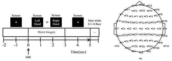
Figure 1.
GIGAScience database experiment for MI-EEG classification (left vs. right hand). (Left) Trial timing: A marker appears onscreen; after two seconds, an instruction is shown to the patient, asking them to imagine moving either their left or right hand. The instruction stays onscreen for three seconds before disappearing. (Right) Spatial EEG montage: electrodes are placed starting at the left frontal nodes and continuing through a serpent pattern until they reach the back, at which point they go back to the front and down the center until they reach the CPZ node (10-10 system).
Preprocessing: Signals were preprocessed before training. An average reference was utilized. Notably, we re-referenced the average after including the initial reference, ensuring the data’s full rank [60]. Then, a fifth-order Butterworth bandpass filter (4–40 Hz) was applied. As the database focuses on motor imagery, rather than higher mental activity like multisensory information integration, most of the information can be found throughout three frequency bands: Theta (4–8 Hz), Alpha (8–13 Hz), and Beta (13–32 Hz) [61,62], while the Gamma rhythm (40 Hz and above) is usually omitted [63]. Afterward, signals are downsampled from 512 Hz to 128 Hz for consistent results between DL models [38,39]. Lastly, only the motor imagery time window is used, as denoted in Figure 1. A summarized version of this preprocess can be seen in Figure 2.
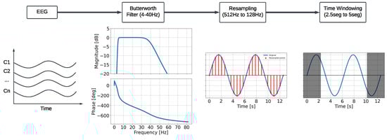
Figure 2.
EEG preprocessing scheme for MI-EEG classification.
Additionally, subjects were asked to complete a physiological questionnaire during the MI experiment. Before beginning the MI experiment, subjects answered 15 personal questions concerning, for example, age, sex, BCI experience, or any recent consumption of coffee, alcohol, or cigarettes. After every run, subjects answered another ten questions about their mood and expected performance. Finally, after the MI experiment, subjects had to answer four questions regarding their thoughts on the experiment and overall personal performance. In total, each subject answered 69 questions. Questions relating to how the patient felt were answered on a scale from one to five, while open questions such as age or expected performance were answered numerically without decimals. However, not all questions were utilized in this study. Shannon’s entropy, as presented in Equation (1),
was measured for each of the Q questions, , and , correctly encoded and normalized between , along with the R subjects to find the ones who provided the most expected information, with the response histogram giving an estimate of . This enabled us to remove cases in which answers had a probability density with low variance (and, by proxy, little discriminant information), such as handedness. Figure 3 illustrates a significant decline in entropy following the initial 31 questions, arranged from the highest entropy to the lowest entropy, indicating that there are questions with styielded considerably less informational value. As a result, only questions with entropy above or equal to the 25th percentile were selected for this study. This then totaled 52 out of the 69 available questions (see Table A1).
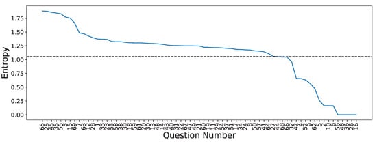
Figure 3.
Shannon’s entropy for the GIGAScience database questionnaire answers. Questions were sorted by their entropy value in decreasing order. The dotted line shows the selected threshold (25th percentile) for selecting questions.
3.2. Subject-Dependent MI-EEG Classification Using Deep Learning
Let be a subject-dependent input–output MI-EEG dataset, gathering N trials, time samples, C channels, and MI-classes ( for the GIGAScience dataset). To optimize meaningful spatial–temporal–spectral patterns in EEG from a given and decrease noise for the improved prediction of MI classes, a DL approach can be employed as follows:
L stands for the number of layers, and
where is a given non-linear activation function, is the l-th feature map , holds the weights and bias of proper size, stands for the number of filters, and collects the network parameters. Furthermore, ⊗ represents the tensor product operator for fully connected, convolutional, or recurrent layers.
Then, an optimization problem can be formulated as follows:
where is a given loss function, i.e., cross-entropy. In addition, a gradient descent-based framework using back-propagation is employed to optimize the parameter set [64]:
where a sample mean estimation is used to approximate the expected value, and an autodiff-based approach computes the gradient ( is a learning rate).
Here, the following MI-EEG DL networks will be considered:
- EEGNet [36]: The process begins with a temporal convolution, which is followed by a depthwise layer that serves as a spatial representation for each filter produced at the previous stage. Afterward, an exponential linear activation function (ELU) is used before an average pooling and a dropout to help minimize overfitting. Next, it applies separable convolution, which is followed by another ELU activation and an average pooling. Lastly, a second dropout layer precedes the flattening and classification stages. Batch normalization is always performed immediately after each convolutional layer.
- KREEGNet [38]: Similar to EEGNet, it uses a Gaussian kernel after batch normalization to extract the connectivity between EEG channels. A delta kernel is implemented on the label data, and a centered kernel alignment (CKA)-based regularization between connectivities and label data is added as a penalty to the straightforward cross-entropy.
- KCS-FCNet [39]: A single convolutional stage occurs before a Gaussian kernel is utilized to measure EEG connectivity. These are then run through an average pooling layer before batch normalization and classification. Interestingly enough, a dropout step is performed between the flatten layer and the dense layer.
- ShallowConvNet [65]: It performs two consecutive convolutions and then proceeds with batch normalization and square activation. After that, average pooling is achieved before logarithmic activation and dropout. Finally, a layer of flattening and density is applied for classification.
- DeepConvNet [19]: The system employs two convolutional layers sequentially, followed by batch normalization and ELU activation. Then, max pooling and dropout are employed before another convolutional layer and batch normalization. Another set of ELU activation, max pooling, and dropouts is performed before a final convolution and batch normalization. Finally, another ELU, max pooling, and dropout are performed before classifying.
- TCFusionNet [37]: Similar to EEGNet, it employs a sequence of residual blocks to gather extra data prior to classification. Each residual block is comprised of dilated convolution, followed by batch normalization, ELU, and dropout twice. In parallel, convolution is performed and then concatenated to the output of the residual block. Before the flattened features from the separable convolution stage are flattened and joined, multiple residual blocks are put in place in a cascading fashion. Finally, a dense layer is used for classification.
Figure 4 shows a summarized visual guide of the different MI-EEG architectures.
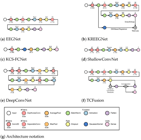
Figure 4.
MI-EEG classification models based on deep learning. Softmax activation is always used after the final dense layer for label prediction. Nodes symbolize the different layers with arrows showcasing their connections. Colors are used to differentiate between layer types while outline is used to differentiate specific layers within the same family.
3.3. Layer-Wise Class Activation Maps for Explainable MI-EEG Classification
Layer-wise class-activation mapping (Layer-CAM) is a powerful technique for DL interpretability that addresses the need to understand how neural networks make decisions [55]. By generating heatmaps that highlight the most relevant regions in an input image, Layer-CAM allows researchers to visualize the specific features contributing to the network’s predictions at various layers. Unlike traditional CAM methods, Layer-CAM captures class-discriminative regions at intermediate layers, providing a more detailed and multilevel perspective on feature importance. Moreover, it supports model refinement by highlighting misinterpreted regions. Here, we implement Layer-CAM within a MI-EEG framework by modeling each EEG trial as an image that holds C rows and columns. Then, let be the upsampled MI-EEG CAM of a given input trial, , for the k-th class () in the l-th layer (), defined as follows:
where is an up-sampling function, represents the network activation map for the l-th layer regarding the p-th filter and the k-th MI class, and gathers the corresponding CAM weight matrix with respect to the k-th output score. By utilizing the backward class-specific gradients, Layer-CAM computes each as follows:
with being the k-th class score holding a linear activation.
To highlight relevant spatial and temporal EEG inputs while avoiding spurious CAM artifacts, we normalize the EEG Layer-CAM as follows:
where is an all-ones column vector of the proper size. Afterward, an EEG explanation map, , can be computed from trial as follows:
Lastly, the gain measure (see Equation (10)) is used to assess the importance of different regions in an input EEG that contribute to the model’s decision for a specific class [66]:
3.4. Questionnaire-MI Performance Canonical Correlation Analysis (QMIP-CCA)
Let us consider the questionnaire matrix holding Q informative MI-EEG questions (see Section 3.1) along R subjects. In turn, let be an MI-EEG classification performance matrix, holding the following measures:
where , , , and stand for true positive, true negative, false positive, and false negative, respectively. Notably, the accuracy, the area under the curve (AUC), and the Kappa (see Equations (11)–(13)) quantify the DL MI-EEG classification performance [64]. We also compute the aforementioned MI performance measures using, as input, the explanation maps in Equation (9). Consequently, for a given DL model.
Next, we propose to compute the questionnaire and MI-performance inter-subject matching matrices, and , as follows:
with and ; , and . The kernel function is set as a Gaussian similarity with bandwidth , which is found by taking the median of the Euclidean distances between the kernel input samples as follows: and
Lastly, to code the questionnaire and MI-performance non-linear matching between subjects by projecting them into a higher-dimensional feature space using , we employ the following CCA-based optimization [67]:
The constraint optimization problem in Equation (16), with and , can be solved via the following generalized eigenvalue-based solution:
The weights in and code the relevance of the Q questions and the A MI performance measures to match the multimodal feature spaces. Additionally, the basis matrices and allow us to compute the subspaces and and the relevance vectors , yielding the following:
with being the softmax function.
3.5. Multimodal and Explainable Deep Learning Implementation Details
Our multimodal and explainable deep learning (MEDL) pipeline can be summarized as in Figure 5. First, the GiGaScience dataset is used to train a subject-dependent DL classifier based on convolutional networks (see Section 3.2 and Figure 4 for DL architectures). EEG signals are encoded as a set of single-channel images of size for all architectures. Then, a Layer-CAM-based approach is carried out to visualize and quantify the MI-EEG explainability (see Section 3.3). Lastly, a QMIP-CCA approach is used to compute the questionnaire and the MI-EEG performance matching (see Section 3.4).
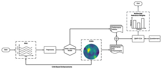
Figure 5.
Experiment’s workflow using MEDL. Each model generates CAMs that are then used to enhance the original EEG input. Model and CAM-based performance measures, along with the questionnaire, are used to perform multimodal analysis via QMIP-CCA.
We trained each model using TensorFlow version 2.17.0 and Keras version 3.2.1. All tests were performed in Kaggle notebook environments. These environments provide two Tesla (NVIDIA, Santa Clara, CA, USA) T4 GPUs with 15 GB of VRAM, 30 GB of RAM, an Intel Xeon CPU @ 2 GHz with two threads per core, and two sockets per core. We implemented a fix for 500 epochs, terminated the process on Nan, and reduced the learning rate on plateaus that serve as callbacks. Also, the Adam optimizer and the categorical cross-entropy-based loss were fixed. Table 1 summarizes the DL hyperparameters employed. Any values not mentioned were fixed regarding TensorFlow’s default selection. The approaches were trained utilizing the same hyperparameters as their original work. Furthermore, stratified cross-validation was implemented for five folds, primarily measuring accuracy to determine the best model for each subject. For this research, the best fold was selected for each model and subject to generate the best CAM possible for each subject and network. Additionally, all notebooks and codes are publicly available at https://github.com/Marcos-L/CAMs-Enhancements (accessed on 22 November 2024).

Table 1.
Subject-dependent MI-EEG classification DL hyperparameters.
For each model, CAMs were extracted from the first temporal convolutional layer. This was done because every architecture uses spatial convolutions for the second convolution stage, which reduces the latent representation of the EEG to a single channel. This means that CAMs will only highlight temporal information when generated from the second convolutional stage onward. Figure 5 summarizes our MEDL pipeline.
4. Results
4.1. MI Classification Performance
All six CNN models and the straightforward filter bank CSP approach, CSP for simplicity, were trained, evaluated, and contrasted among themselves based on their cross-validation results. Figure 6 shows the different metrics for each model prior to the CAM-based enhancements. KREEGNet showed the best accuracy and AUC score, while DeepConvNet showed the worst. In general, kernel methods improved upon the baseline EEGNet. Despite having fewer feature extraction layers, ShallowConvNet remained comparable, while CSP and DeepConvNet lost a significant amount of accuracy compared to the other techniques. Moreover, despite its more complex architecture, TCFusion performed almost identically to EEGNet.
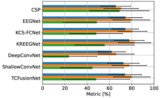
Figure 6.
MI-EEG GiGaScience classification results. Blue: accuracy; orange: AUC; green: Kappa.
Furthermore, when observing inter-subject accuracy across models, as seen in Figure 7, DeepConvNet’s low performance becomes more apparent. Grouping subjects into three groups based on their classification accuracy on EEGNet (good, mid, and poor), DeepConvNet struggles a lot to properly classify good MI subjects, only ever outperforming EEGNet for the two worst subjects. In contrast, KCS-FCNet, although underperforming for good subjects, remains consistent for mid and poor subjects. Interestingly, ShallowConvNet performs well in the poor-performing group.
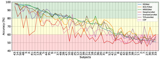
Figure 7.
Inter-subject accuracy results. Subjects are sorted based on EEGNet performance.
Furthermore, additional statistical tests were carried out to judge the consistency of these models. Figure 8a shows the models ranked by performance for each subject, with 1 being the best and 7 being the worst. This clearly shows that CSP and DeepConvNet are the worst models overall, while all other models are consistent with each other. When evaluating the Friedman chi test, in this regard, we obtain a p-value of , further supporting this. Additionally, Figure 8b shows the results of the t-test to judge the similarity between models, which correlates with the ranking results. Finally, Table 2 shows the average ranking and t-test p-value (ignoring the diagonal) for each architecture.
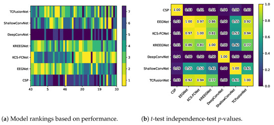
Figure 8.
Models rankings vs. t-test p-values. Subjects are sorted based on EEGNet’s accuracy.
Table 2.
Average rankings and p-values.
Next, Figure 9 shows the distribution of subject performance across groups for each model. It is clear that DeepConvNet yields lower results compared to other models such as EEGNet, which are capable of producing comparable results.
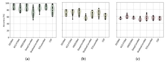
Figure 9.
Group-performing MI-EEG classification results. (a) Subjects with EEGNet accuracy above 80%. (b) Subjects with EEGNet accuracy between 60% and 80%. (c) Subjects with EEGNet accuracy below 60%.
4.2. Explainable MI-EEG Classification Results
Figure 10 displays the average class score percentage gain for EEGNet across performance groups and class labels. This is used to look at how the proposed solution affected the class score. Figure 10a,b shows that the well- and mid-performing groups are biased towards a specific class, with only the poorly performing subjects presenting improvements for both. In contrast, ShallowConvNet’s percentage gains, presented in Figure 11, consistently show that all groups improve for both classes. On the other hand, TCFusion barely shows any gain at all. Figure 12 shows both well- and mid-performing groups only experiencing tiny amounts of improvement when compared to the other two models. The only group to have achieved substantial improvements is the poorly performing one, but only for right-hand MI.
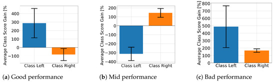
Figure 10.
Class score percentage gain per MI class for EEGNet.
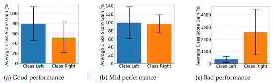
Figure 11.
Class score percentage gain per MI class for ShallowConvNet.
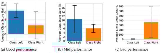
Figure 12.
Class score percentage gain per MI class for TCFusion.
When examining the spatial location of the highlighted features, we generated topomaps from the CAMs by averaging their values across time and trials per class and true label. These topomaps were then normalized among each other, and finally, cubic interpolation was performed to achieve a continuous image [68]. As seen in the CAMs used per class, it is possible to observe a pattern emerging. Figure 13a,c shows the average topomaps for well- and poorly performing subjects. The well-performing subject has the most important features located in the right sensorimotor area, with no information being highlighted on the left side. Then, the model learns the features related to one class and classifies the other whenever the information in this area is non-conclusive, which explains the bias presented by the percentage gain. In contrast, the poor-performing subject displays information highlighted throughout their head, with both classes highlighting nearly identical regions. However, subjects with average performance, like the one shown in Figure 13b, appear to mix the two. The most important information is found in the sensorimotor area for one side, while the rest of the EEG is disrupted due to the noise. This behavior is consistent between models as shown in Figure 14 and Figure 15, except for TCFusion, as presented in Figure 16, which generates spatially noisy CAMs.
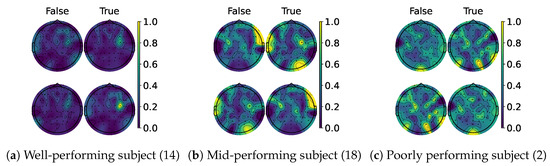
Figure 13.
Topomaps of EEGNet. The top row shows the maps for the left-hand class, while the bottom row shows the same for the right-hand class. The topomaps are min–max-normalized horizontally.
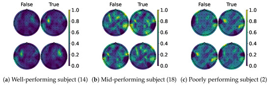
Figure 14.
Topomaps of KREEGNet. The top row shows the maps for the left-hand class, while the bottom row shows the same for the right-hand class. The topomaps are min–max-normalized horizontally.
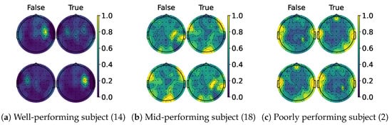
Figure 15.
Topomaps of ShallowConvNet. The top row shows the maps for the left-hand class, while the bottom row shows the same for the right-hand class. The topomaps are min–max-normalized horizontally.
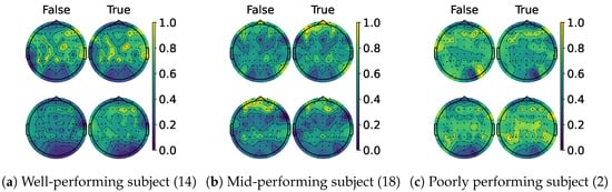
Figure 16.
Topomaps of TCFusion. The top row shows the maps for the left-hand class, while the bottom row shows the same for the right-hand class. The topomaps are min–max-normalized horizontally.
Additionally, Figure 17 shows the improvement distribution for the different models across all three groups for the best fold across strategies. Noticeably, ShallowConvNet achieves consistently positive improvements, as opposed to other models, which achieve a mix of improvements and losses. However, in general, all models tend to show improvements or at least remain the same, with a median improvement close to zero across all three groups and some edge cases showing massive losses. The only exception to this rule is TCFusion, which consistently loses accuracy across all three groups. Furthermore, Table 3 shows the average change in accuracy for all models across all subjects and all folds. All models see minor changes, with KREEGNet seeing the best improvement overall, but with high variability, and ShallowConvNet showing minor losses.
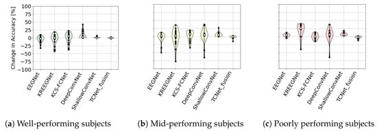
Figure 17.
Violin plot of change in accuracy after CAM enhancements for different subject groups across DL models.
Table 3.
MI-EEG classification performance comparison: ACC vs. CAM-enhanced ACC. Average ACC ± standard deviation.
Finally, when model rankings and similarity were re-evaluated, they changed greatly. Figure 18a shows the rankings after enhancements, with subjects sorted the same way as Figure 7 and Figure 8. Here, we can observe how the kernel-based strategies drop considerably, with the pure convolutional models of ShallowConvNet and DeepConvNet becoming much better. Additionally, Figure 18b shows how these results become extremely different amongst the different architectures, with only the kernel-based model remaining somewhat similar between them, as well as EEGNet with TCFusion. Finally, Table 4 shows the average ranking and p-values calculated in the same manner as Table 2.
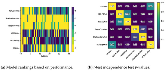
Figure 18.
Models rankings vs. t-test p-values after CAM enhancements.
Table 4.
Average rankings and p-values after CAM enhancements.
4.3. Questionnaire and MI-EEG Performance Relevance Analysis Results
Figure 19 shows the CCA and our kernel-based CCA variant relevance analysis for the questionnaire data compared to the MI-EEG performance measures. While linear CCA only yields a single correlation for the “How do you feel?” question, which spans from “very good” to “very bad” or “tired”, our approach reveals a more diverse range of questions. The questions that have a relevance value greater than or equal to 0.5 pertain to the patient’s overall feelings across various runs, with the exception of a single question with an expected relevance of . On the other hand, CCA reveals that DeepConvNet’s kappa after improvements is the most important MI performance. In contrast, kernel-based CCA shows that EEGNet’s accuracy after improvements and kappa after improvements are the most important features.
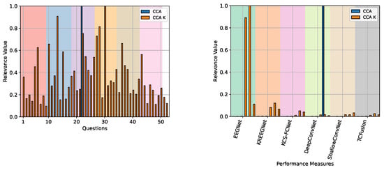
Figure 19.
The QMIP-CCA relevance analysis results are derived from the multimodal GiGaScience dataset. Questionnaire (left) and MI-EEG classification performance measures (right) are studied. Linear CCA and our kernel-based CA enhancement are presented. Background colors for the questionnaire divide the questions into Pre-MI (red), Runs 1 through 5 (blue, purple, yellow, brown, and pink), and Post-MI (white). For the MI-EEG classification measures, colors show the corresponding DL model.
When QMIP-CCA was evaluated across subject groups, a pattern emerged with respect to the relevance of performance measures. For the good and mid groups, presented in Figure 20 and Figure 21, respectively, CAM-enhanced measures achieved low relevance values, with average scores of and respectively. Meanwhile, for the poor performance group, presented in Figure 22, these scores achieved an average value of .
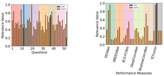
Figure 20.
The QMIP-CCA relevance analysis for the good performance group. Questionnaire (left) and MI-EEG classification performance measures (right).
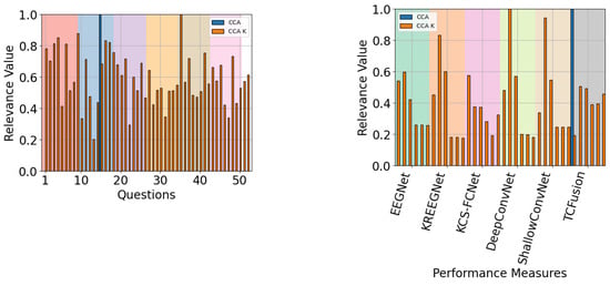
Figure 21.
The QMIP-CCA relevance analysis for the mid-performance group. Questionnaire (left) and MI-EEG classification performance measures (right).
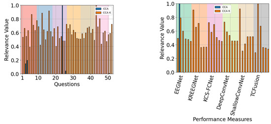
Figure 22.
The QMIP-CCA relevance analysis for the poor-performance group. Questionnaire (left) and MI-EEG classification performance measures (right).
Finally, when the model-specific results were analyzed, most models tended to behave the same: with measures after gains being the most relevant (see Figure 23 and Figure 24). The only exception to this rule is TCFusion, as shown in Figure 25, which does attribute considerable relevance to accuracy before enhancements. This further correlates with the results shown in Section 4.2, suggesting that simple shallow models obtain more information from enhanced features. Additionally, questionnaire relevancy achieves similar results to the ones presented for all models in Figure 19, with questions relating to the feeling and perception of the experiment having high relevancy across all models.
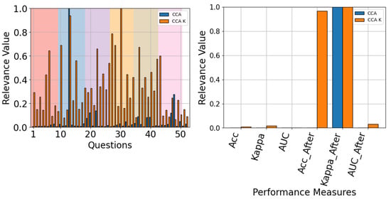
Figure 23.
The QMIP-CCA relevance analysis for EEGNet. Questionnaire (left) and MI-EEG classification performance measures (right).
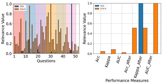
Figure 24.
The QMIP-CCA relevance analysis for ShallowConvNet. Questionnaire (left) and MI-EEG classification performance measures (right).
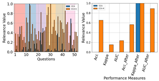
Figure 25.
The QMIP-CCA relevance analysis for TCFusion. Questionnaire (left) and MI-EEG classification performance measures (right).
5. Discussion
The results highlight the trade-offs between model complexity and performance in subject-specific MI-EEG classification. While deeper networks like DeepConvNet showed potential for extracting complex features, their high parameter count likely contributed to overfitting [69]. This highlights the importance of balancing complexity with regularization, particularly in tasks with limited and noisy training data. In contrast, Kernel-based models such as KREEGNet and KCS-FCNet demonstrated strong performance, suggesting that kernel methods are particularly effective in MI-EEG classification. Interestingly, ShallowConvNet’s simplicity proved advantageous for subject-dependent classification, highlighting that fewer features may suffice in noisy conditions.
Furthermore, the statistical tests corroborated the consistency of these findings, with models like EEGNet and KREEGNet maintaining robust performance rankings. Additionally, the Friedman chi-square test and t-test results suggest consistency between models, meaning subject groups should remain consistent across strategies. Overall, these findings suggest that simpler and more regularized architectures are better suited for subject-specific MI-EEG classification tasks. In contrast, deeper models require improved optimization techniques to mitigate overfitting [47].
When the models were evaluated after CAM-based feedback, the results highlight differences in how the models’ behavior changes due to the CAM-based enhancements. EEGNet shows class-specific biases for well- and mid-performing subjects, as shown in Figure 10, while poor-performing subjects see an improvement for both. This suggests that the model learns features corresponding to a single class for well- and mid-performing subjects, while models for poor-performing subjects achieve better generalizations. This is further supported by the topomaps shown in Figure 13, which shows most of the energy localized to one side of the head, hence explaining the bias for one specific class [70].
In contrast, ShallowConvNet achieves improvements for both classes across all three groups, implying that shallow and purely convolutional strategies achieve better generalization and benefits more from CAM-based feedback. Although ShallowConv’s topomaps, shown in Figure 15, also localize information on one side, it also detects some relevant features on the opposite one, making it more robust to class bias. On the other hand, TCFusion’s minimal gain (Figure 12) suggests that it is less effective at leveraging the discriminative power of CAMs, likely due to how noisy they are, as seen in Figure 16. This aligns with its overall negative trend in accuracy improvement, as seen in Figure 17. Additionally, the re-evaluated statistical and ranking tests show that pure convolutional strategies now outperform the kernel-based ones. This suggests that the non-linear mapping greatly influences our feedback approach’s efficacy, making this strategy more consistent in architectures more reliant on convolutional layers.
Then, the ability of a model to effectively leverage CAM-based enhancements appears to depend on its design’s complexity. Purely convolutional strategies like ShallowConvNet and DeepConvNet demonstrate promising improvements, with models like EEGNet suffering from class bias, likely indicating poor generalization. Conversely, TCFusion and kernel-based strategies, although remaining consistent overall, become comparatively worse, hence suggesting that architecture complexity influences the efficacy of CAM enhancements.
In turn, the QMIP-CCA results suggest a significant relationship between participants’ self-reported feelings during the experiment and the performance improvements observed in MI-EEG measures. The diversity of relevant questions identified via the kernel-based CCA approach, particularly those related to overall feelings during the experiment, indicates that the improvements produced via the CAM feedback are linked to how comfortable or relaxed the subject feels during the experiment [71].
The finding that CAM-enhanced measures become more relevant as regular performance decreases highlights the potential importance of feedback mechanisms in improving MI performance, especially for participants whose baseline performance is lower. The increased relevance of CAM-enhanced measures for the poor performance group could suggest that these participants benefit more from the feedback interventions than those with better baseline performance. Additionally, the fact that the questionnaire relevancy did not show a clear pattern across different subject groups implies that factors such as baseline performance do not necessarily correlate with how subjects perceive or respond to the experiment.
Lastly, model-specific results offer further insights into how different models interact with the enhancements. Most strategies find a higher correlation between the physiological questionnaire and the CAM-based results than with the pre-feedback ones. This indicates that the behavior and personal traits of a patient will influence the potency feedback strategies might provide, and by extension, they might also indicate a connection with the spatiotemporal location of relevant features. However, the behavior of TCFusion, which ascribes greater relevance to pre-CAM accuracy, points to the idea that architecture complexity has a great influence on which kinds of features become relevant to the model, as these features do not benefit from further MI-EEG classification enhancement.
6. Conclusions
We have presented a multimodal and explainable deep learning (MEDL) framework for MI-EEG classification, combining class activation maps (CAMs) and canonical correlation analysis (CCA) to improve classification accuracy and enhance the interpretability of MI-EEG-based models. The proposed approach involves evaluating various deep-learning approaches for MI-EEG classification. Additionally, the use of CAM-based methods successfully highlighted relevant patterns crucial for decision-making in motor imagery classification. Using the Questionnaire-MI Performance Canonical Correlation Analysis (QMIP-CCA) framework gave us a new way to connect subjective questionnaire data with MI-EEG classification performance. This showed us important physiological and cognitive factors that affect how well the models explain things and how accurate the classifications are. ShallowConvNet, in particular, showed the most consistent improvements across different performance groups, proving to be more robust in handling noisy EEG data for poorly performing subjects.
For future work, we aim to extend the multimodal approach by integrating more diverse physiological and environmental data sources to further enhance model accuracy and interpretability [72]. Additionally, exploring more advanced deep learning methods, such as transformer-based networks, and more sophisticated attention mechanisms could improve the robustness of CAMs in capturing relevant EEG features across a wider variety of tasks [73]. Another direction would be the development of subject-independent models to address inter-subject variability, which remains a significant challenge in EEG classification [45].
Author Contributions
Conceptualization, M.L.-A., A.M.Á.-M. and G.C.-D.; data curation, M.L.-A.; methodology, M.L.-A., A.M.Á.-M. and D.C.-P.; project administration, A.M.Á.-M. and Á.Á.O.-G.; supervision, A.M.Á.-M., Á.Á.O.-G. and G.C.-D.; resources, M.L.-A. and D.C.-P. All authors have read and agreed to the published version of the manuscript.
Funding
Funding was provided under grants through the following projects: “Sistema de monitoreo automático para la evaluación clínica de infantes con alteraciones neurológicas motoras mediante el análisis de volumetría cerebral y patrón de marcha” (Code 1110-897-84907 CTO 706-2021, CONV. 897-2021), supported by MINCIENCIAS; and for A. Alvarez and G. Castellanos, thanks to the project “Sistema de integración de EEG, ECG y SpO2 para seguimiento de neonatos en unidad de cuidados intensivos del Hospital Universitario de Caldas - SES HUC”, Hermes 57414, funded by Universidad Nacional de Colombia.
Institutional Review Board Statement
Not applicable.
Informed Consent Statement
Not applicable.
Data Availability Statement
The publicly available dataset analyzed in this study and our Python codes can be found at https://github.com/Marcos-L/CAMs-Enhancements (accessed on 22 October 2024).
Conflicts of Interest
The authors declare no conflicts of interest.
Appendix A. Additional Results
Table A1.
Questionnaire questions selected with their respective entropy value.
Table A1.
Questionnaire questions selected with their respective entropy value.
| Set | Question | Answer Type | Entropy |
|---|---|---|---|
| Pre-MI | Time slot | (1 = 9:30/2 = 12:30/3 = 15:30/4 = 19:00) | 1.373 |
| Age | (number) | 1.774 | |
| How long did you sleep? | (1 = less than 4 h/2=5 – 6 h/3 = 6 –7 h/4 = 7 –8/ 5 = more than 8) | 1.485 | |
| Did you drink coffee within the past 24 h | (0 = no, number = hours before) | 1.172 | |
| How do you feel? | Relaxed 1 2 3 4 5 Anxious | 1.218 | |
| How do you feel? | Exciting 1 2 3 4 5 Boring | 1.429 | |
| How do you feel? | Very good 1 2 3 4 5 Very bad or tired | 1.291 | |
| How do you feel? | Very good 1 2 3 4 5 Very bad or tired | 1.277 | |
| The BCI performance (accuracy) expected? | % | 1.754 | |
| Run 1 | How do you feel? | Relaxed 1 2 3 4 5 Anxious | 1.186 |
| How do you feel? | Exciting 1 2 3 4 5 Boring | 1.305 | |
| How do you feel? | High 1 2 3 4 5 Low | 1.223 | |
| How do you feel? | Very good 1 2 3 4 5 Very bad or tired | 1.301 | |
| How do you feel? | Very good 1 2 3 4 5 Very bad or tired | 1.247 | |
| Have you nodded off (slept a while) during this run? | (0 = no/number = how many times) | 1.253 | |
| Was it easy to imagine finger movements? | Easy 1 2 3 4 5 Difficult | 1.368 | |
| How many trials you missed? | (0 = no/number = how many times) | 1.179 | |
| The BCI performance (accuracy) expected? | % | 1.879 | |
| Run 2 | How do you feel? | Relaxed 1 2 3 4 5 Anxious | 1.062 |
| How do you feel? | Exciting 1 2 3 4 5 Boring | 1.397 | |
| How do you feel? | High 1 2 3 4 5 Low | 1.217 | |
| How do you feel? | Very good 1 2 3 4 5 Very bad or tired | 1.295 | |
| How do you feel? | Very good 1 2 3 4 5 Very bad or tired | 1.254 | |
| Was it easy to imagine finger movements? | Easy 1 2 3 4 5 Difficult | 1.371 | |
| How many trials you missed? | (0 = no/number = how many times) | 1.185 | |
| The BCI performance (accuracy) expected? | % | 1.846 | |
| Run 3 | How do you feel? | Relaxed 1 2 3 4 5 Anxious | 1.205 |
| How do you feel? | Exciting 1 2 3 4 5 Boring | 1.324 | |
| How do you feel? | High 1 2 3 4 5 Low | 1.313 | |
| How do you feel? | Very good 1 2 3 4 5 Very bad or tired | 1.256 | |
| How do you feel? | Very good 1 2 3 4 5 Very bad or tired | 1.144 | |
| Was it easy to imagine finger movements? | Easy 1 2 3 4 5 Difficult | 1.263 | |
| How many trials you missed? | (0 = no/number = how many times) | 1.055 | |
| The BCI performance (accuracy) expected? | % | 1.859 | |
| Run 4 | How do you feel? | Relaxed 1 2 3 4 5 Anxious | 1.250 |
| How do you feel? | Exciting 1 2 3 4 5 Boring | 1.287 | |
| How do you feel? | High 1 2 3 4 5 Low | 1.249 | |
| How do you feel? | Very good 1 2 3 4 5 Very bad or tired | 1.161 | |
| How do you feel? | Very good 1 2 3 4 5 Very bad or tired | 1.201 | |
| Was it easy to imagine finger movements? | Easy 1 2 3 4 5 Difficult | 1.329 | |
| How many trials you missed? | (0 = no/number = how many times) | 1.212 | |
| The BCI performance (accuracy) expected? | % | 1.833 | |
| Run 5 | How do you feel? | Relaxed 1 2 3 4 5 Anxious | 1.154 |
| How do you feel? | Exciting 1 2 3 4 5 Boring | 1.324 | |
| How do you feel? | High 1 2 3 4 5 Low | 1.304 | |
| How do you feel? | Very good 1 2 3 4 5 Very bad or tired | 1.223 | |
| How do you feel? | Very good 1 2 3 4 5 Very bad or tired | 1.304 | |
| Was it easy to imagine finger movements? | Easy 1 2 3 4 5 Difficult | 1.469 | |
| How many trials you missed? | (0 = no/number = how many times) | 1.108 | |
| The BCI performance (accuracy) expected? | % | 1.883 | |
| Post-MI | How was this experiment? | Good 1 2 3 4 5 Bad | 1.250 |
| The BCI performance (accuracy) of whole data expected? | % | 1.665 |
References
- UNESCO; International Center for Engineering Education. Engineering for Sustainable Development: Delivering on the Sustainable Development Goals; United Nations Educational, Scientific, and Cultural Organization: Paris, France; International Center for Engineering Education Under the Auspices of UNESCO: Beijing, China; Compilation and Translation Press: Beijing, China, 2021. [Google Scholar]
- Mayo Clinic Editorial Staff. EEG (Electroencephalogram). 2024. Available online: https://www.mayoclinic.org/tests-procedures/eeg/about/pac-20393875 (accessed on 17 August 2024).
- Altaheri, H.; Muhammad, G.; Alsulaiman, M.; Amin, S.U.; Altuwaijri, G.A.; Abdul, W.; Bencherif, M.A.; Faisal, M. Deep learning techniques for classification of electroencephalogram (EEG) motor imagery (MI) signals: A review. Neural Comput. Appl. 2023, 35, 14681–14722. [Google Scholar] [CrossRef]
- Ramadan, R.A.; Altamimi, A.B. Unraveling the potential of brain-computer interface technology in medical diagnostics and rehabilitation: A comprehensive literature review. Health Technol. 2024, 14, 263–276. [Google Scholar] [CrossRef]
- Abidi, M.; De Marco, G.; Grami, F.; Termoz, N.; Couillandre, A.; Querin, G.; Bede, P.; Pradat, P.F. Neural correlates of motor imagery of gait in amyotrophic lateral sclerosis. J. Magn. Reson. Imaging 2021, 53, 223–233. [Google Scholar] [CrossRef] [PubMed]
- Zhang, H.; Zhao, M.; Wei, C.; Mantini, D.; Li, Z.; Liu, Q. EEGdenoiseNet: A benchmark dataset for deep learning solutions of EEG denoising. J. Neural Eng. 2021, 18, 056057. [Google Scholar] [CrossRef] [PubMed]
- Saini, M.; Satija, U.; Upadhayay, M.D. Wavelet based waveform distortion measures for assessment of denoised EEG quality with reference to noise-free EEG signal. IEEE Signal Process. Lett. 2020, 27, 1260–1264. [Google Scholar] [CrossRef]
- Tsuchimoto, S.; Shibusawa, S.; Iwama, S.; Hayashi, M.; Okuyama, K.; Mizuguchi, N.; Kato, K.; Ushiba, J. Use of common average reference and large-Laplacian spatial-filters enhances EEG signal-to-noise ratios in intrinsic sensorimotor activity. J. Neurosci. Methods 2021, 353, 109089. [Google Scholar] [CrossRef]
- Croce, P.; Quercia, A.; Costa, S.; Zappasodi, F. EEG microstates associated with intra-and inter-subject alpha variability. Sci. Rep. 2020, 10, 2469. [Google Scholar] [CrossRef] [PubMed]
- Saha, S.; Baumert, M. Intra-and inter-subject variability in EEG-based sensorimotor brain computer interface: A review. Front. Comput. Neurosci. 2020, 13, 87. [Google Scholar] [CrossRef]
- Maswanganyi, R.C.; Tu, C.; Owolawi, P.A.; Du, S. Statistical evaluation of factors influencing inter-session and inter-subject variability in eeg-based brain computer interface. IEEE Access 2022, 10, 96821–96839. [Google Scholar] [CrossRef]
- Blanco-Diaz, C.F.; Antelis, J.M.; Ruiz-Olaya, A.F. Comparative analysis of spectral and temporal combinations in CSP-based methods for decoding hand motor imagery tasks. J. Neurosci. Methods 2022, 371, 109495. [Google Scholar] [CrossRef] [PubMed]
- Wang, B.; Wong, C.M.; Kang, Z.; Liu, F.; Shui, C.; Wan, F.; Chen, C.P. Common spatial pattern reformulated for regularizations in brain–computer interfaces. IEEE Trans. Cybern. 2020, 51, 5008–5020. [Google Scholar] [CrossRef] [PubMed]
- Galindo-Noreña, S.; Cárdenas-Peña, D.; Orozco-Gutierrez, A. Multiple Kernel Stein Spatial Patterns for the Multiclass Discrimination of Motor Imagery Tasks. Appl. Sci. 2020, 10, 8628. [Google Scholar] [CrossRef]
- Geng, X.; Li, D.; Chen, H.; Yu, P.; Yan, H.; Yue, M. An improved feature extraction algorithms of EEG signals based on motor imagery brain-computer interface. Alex. Eng. J. 2022, 61, 4807–4820. [Google Scholar] [CrossRef]
- Chollet, F. Deep Learning with Python; Manning: Shelter Island, NY, USA, 2017. [Google Scholar]
- Collazos-Huertas, D.F.; Álvarez-Meza, A.M.; Castellanos-Dominguez, G. Image-based learning using gradient class activation maps for enhanced physiological interpretability of motor imagery skills. Appl. Sci. 2022, 12, 1695. [Google Scholar] [CrossRef]
- Rakhmatulin, I.; Dao, M.S.; Nassibi, A.; Mandic, D. Exploring Convolutional Neural Network Architectures for EEG Feature Extraction. Sensors 2024, 24, 877. [Google Scholar] [CrossRef] [PubMed]
- Schirrmeister, R.T.; Springenberg, J.T.; Fiederer, L.D.J.; Glasstetter, M.; Eggensperger, K.; Tangermann, M.; Hutter, F.; Burgard, W.; Ball, T. Deep learning with convolutional neural networks for EEG decoding and visualization. Hum. Brain Mapp. 2017, 38, 5391–5420. [Google Scholar] [CrossRef]
- Li, F.; He, F.; Wang, F.; Zhang, D.; Xia, Y.; Li, X. A novel simplified convolutional neural network classification algorithm of motor imagery EEG signals based on deep learning. Appl. Sci. 2020, 10, 1605. [Google Scholar] [CrossRef]
- Liu, J.; Wu, G.; Luo, Y.; Qiu, S.; Yang, S.; Li, W.; Bi, Y. EEG-based emotion classification using a deep neural network and sparse autoencoder. Front. Syst. Neurosci. 2020, 14, 43. [Google Scholar] [CrossRef] [PubMed]
- Chowdary, M.K.; Anitha, J.; Hemanth, D.J. Emotion recognition from EEG signals using recurrent neural networks. Electronics 2022, 11, 2387. [Google Scholar] [CrossRef]
- Ma, Y.; Song, Y.; Gao, F. A novel hybrid CNN-transformer model for EEG motor imagery classification. In Proceedings of the 2022 International Joint Conference on Neural Networks (IJCNN), Padua, Italy, 18–23 July 2022; IEEE: New York, NY, USA, 2022; pp. 1–8. [Google Scholar]
- Li, X.; Xiong, H.; Li, X.; Wu, X.; Zhang, X.; Liu, J.; Bian, J.; Dou, D. Interpretable deep learning: Interpretation, interpretability, trustworthiness, and beyond. Knowl. Inf. Syst. 2022, 64, 3197–3234. [Google Scholar] [CrossRef]
- Bhardwaj, H.; Tomar, P.; Sakalle, A.; Ibrahim, W. Eeg-based personality prediction using fast fourier transform and deeplstm model. Comput. Intell. Neurosci. 2021, 2021, 6524858. [Google Scholar] [CrossRef] [PubMed]
- Cho, H.; Ahn, M.; Ahn, S.; Kwon, M.; Jun, S.C. EEG datasets for motor imagery brain–computer interface. GigaScience 2017, 6, gix034. [Google Scholar] [CrossRef] [PubMed]
- Rahman, A.U.; Tubaishat, A.; Al-Obeidat, F.; Halim, Z.; Tahir, M.; Qayum, F. Extended ICA and M-CSP with BiLSTM towards improved classification of EEG signals. Soft Comput. 2022, 26, 10687–10698. [Google Scholar] [CrossRef]
- Jin, J.; Xiao, R.; Daly, I.; Miao, Y.; Wang, X.; Cichocki, A. Internal Feature Selection Method of CSP Based on L1-Norm and Dempster–Shafer Theory. IEEE Trans. Neural Netw. Learn. Syst. 2021, 32, 4814–4825. [Google Scholar] [CrossRef]
- Wang, H.; Tang, Q.; Zheng, W. L1-Norm-Based Common Spatial Patterns. IEEE Trans. Biomed. Eng. 2012, 59, 653–662. [Google Scholar] [CrossRef] [PubMed]
- Ang, K.K.; Chin, Z.Y.; Zhang, H.; Guan, C. Filter Bank Common Spatial Pattern (FBCSP) in Brain-Computer Interface. In Proceedings of the 2008 IEEE International Joint Conference on Neural Networks (IEEE World Congress on Computational Intelligence), Hong Kong, China, 1–8 June 2008; pp. 2390–2397. [Google Scholar] [CrossRef]
- Zhang, Y.; Zhou, G.; Jin, J.; Wang, X.; Cichocki, A. Optimizing spatial patterns with sparse filter bands for motor-imagery based brain–computer interface. J. Neurosci. Methods 2015, 255, 85–91. [Google Scholar] [CrossRef] [PubMed]
- Miao, Y.; Jin, J.; Daly, I.; Zuo, C.; Wang, X.; Cichocki, A.; Jung, T.P. Learning common time-frequency-spatial patterns for motor imagery classification. IEEE Trans. Neural Syst. Rehabil. Eng. 2021, 29, 699–707. [Google Scholar] [CrossRef]
- Luo, J.; Gao, X.; Zhu, X.; Wang, B.; Lu, N.; Wang, J. Motor imagery EEG classification based on ensemble support vector learning. Comput. Methods Programs Biomed. 2020, 193, 105464. [Google Scholar] [CrossRef]
- Tibrewal, N.; Leeuwis, N.; Alimardani, M. Classification of motor imagery EEG using deep learning increases performance in inefficient BCI users. PLoS ONE 2022, 17, e0268880. [Google Scholar] [CrossRef]
- Lopes, M.; Cassani, R.; Falk, T.H. Using CNN Saliency Maps and EEG Modulation Spectra for Improved and More Interpretable Machine Learning-Based Alzheimer’s Disease Diagnosis. Comput. Intell. Neurosci. 2023, 2023, 3198066. [Google Scholar] [CrossRef]
- Lawhern, V.J.; Solon, A.J.; Waytowich, N.R.; Gordon, S.M.; Hung, C.P.; Lance, B.J. EEGNet: A compact convolutional neural network for EEG-based brain–computer interfaces. J. Neural Eng. 2018, 15, 056013. [Google Scholar] [CrossRef]
- Musallam, Y.K.; AlFassam, N.I.; Muhammad, G.; Amin, S.U.; Alsulaiman, M.; Abdul, W.; Altaheri, H.; Bencherif, M.A.; Algabri, M. Electroencephalography-based motor imagery classification using temporal convolutional network fusion. Biomed. Signal Process. Control 2021, 69, 102826. [Google Scholar] [CrossRef]
- Tobón-Henao, M.; Álvarez Meza, A.M.; Castellanos-Dominguez, C.G. Kernel-Based Regularized EEGNet Using Centered Alignment and Gaussian Connectivity for Motor Imagery Discrimination. Computers 2023, 12, 145. [Google Scholar] [CrossRef]
- García-Murillo, D.G.; Álvarez Meza, A.M.; Castellanos-Dominguez, C.G. KCS-FCnet: Kernel Cross-Spectral Functional Connectivity Network for EEG-Based Motor Imagery Classification. Diagnostics 2023, 13, 1122. [Google Scholar] [CrossRef]
- Lu, N.; Li, T.; Ren, X.; Miao, H. A deep learning scheme for motor imagery classification based on restricted Boltzmann machines. IEEE Trans. Neural Syst. Rehabil. Eng. 2016, 25, 566–576. [Google Scholar] [CrossRef] [PubMed]
- Mirzaei, S.; Ghasemi, P. EEG motor imagery classification using dynamic connectivity patterns and convolutional autoencoder. Biomed. Signal Process. Control 2021, 68, 102584. [Google Scholar] [CrossRef]
- Hwaidi, J.F.; Chen, T.M. Classification of motor imagery EEG signals based on deep autoencoder and convolutional neural network approach. IEEE Access 2022, 10, 48071–48081. [Google Scholar] [CrossRef]
- Wei, C.S.; Keller, C.J.; Li, J.; Lin, Y.P.; Nakanishi, M.; Wagner, J.; Wu, W.; Zhang, Y.; Jung, T.P. Inter-and intra-subject variability in brain imaging and decoding. Front. Comput. Neurosci. 2021, 15, 791129. [Google Scholar] [CrossRef]
- Alessandrini, M.; Biagetti, G.; Crippa, P.; Falaschetti, L.; Luzzi, S.; Turchetti, C. Eeg-based alzheimer’s disease recognition using robust-pca and lstm recurrent neural network. Sensors 2022, 22, 3696. [Google Scholar] [CrossRef]
- Luo, J.; Wang, Y.; Xia, S.; Lu, N.; Ren, X.; Shi, Z.; Hei, X. A shallow mirror transformer for subject-independent motor imagery BCI. Comput. Biol. Med. 2023, 164, 107254. [Google Scholar] [CrossRef]
- Bang, J.S.; Lee, S.W. Interpretable convolutional neural networks for subject-independent motor imagery classification. In Proceedings of the 2022 10th International Winter Conference on Brain-Computer Interface (BCI), Gangwon-do, Republic of Korea, 21–23 February 2022; IEEE: New York, NY, USA, 2022; pp. 1–5. [Google Scholar]
- Bejani, M.M.; Ghatee, M. A systematic review on overfitting control in shallow and deep neural networks. Artif. Intell. Rev. 2021, 54, 6391–6438. [Google Scholar] [CrossRef]
- Zhang, Y.; Tiňo, P.; Leonardis, A.; Tang, K. A survey on neural network interpretability. IEEE Trans. Emerg. Top. Comput. Intell. 2021, 5, 726–742. [Google Scholar] [CrossRef]
- Onishi, S.; Nishimura, M.; Fujimura, R.; Hayashi, Y. Why Do Tree Ensemble Approximators Not Outperform the Recursive-Rule eXtraction Algorithm? Mach. Learn. Knowl. Extr. 2024, 6, 658–678. [Google Scholar] [CrossRef]
- Hong, Q.; Wang, Y.; Li, H.; Zhao, Y.; Guo, W.; Wang, X. Probing filters to interpret CNN semantic configurations by occlusion. In Proceedings of the Data Science: 7th International Conference of Pioneering Computer Scientists, Engineers and Educators, ICPCSEE 2021, Taiyuan, China, 17–20 September 2021; Proceedings, Part II. Springer: Singapore, 2021; pp. 103–115. [Google Scholar]
- Christoph, M. Interpretable Machine Learning: A Guide for Making Black Box Models Explainable; Leanpub: Victoria, BC, Canada, 2020. [Google Scholar]
- Zhou, B.; Khosla, A.; Lapedriza, A.; Oliva, A.; Torralba, A. Learning Deep Features for Discriminative Localization. In Proceedings of the 2016 IEEE Conference on Computer Vision and Pattern Recognition (CVPR), Las Vegas, NV, USA, 27–30 June 2016; pp. 2921–2929. [Google Scholar] [CrossRef]
- Selvaraju, R.R.; Cogswell, M.; Das, A.; Vedantam, R.; Parikh, D.; Batra, D. Grad-CAM: Visual Explanations from Deep Networks via Gradient-Based Localization. Int. J. Comput. Vis. 2019, 128, 336–359. [Google Scholar] [CrossRef]
- Chattopadhay, A.; Sarkar, A.; Howlader, P.; Balasubramanian, V.N. Grad-CAM++: Generalized Gradient-Based Visual Explanations for Deep Convolutional Networks. In Proceedings of the 2018 IEEE Winter Conference on Applications of Computer Vision (WACV), Lake Tahoe, NV, USA, 12–15 March 2018; IEEE: New York, NY, USA, 2018. [Google Scholar] [CrossRef]
- Jiang, P.T.; Zhang, C.B.; Hou, Q.; Cheng, M.M.; Wei, Y. Layercam: Exploring hierarchical class activation maps for localization. IEEE Trans. Image Process. 2021, 30, 5875–5888. [Google Scholar] [CrossRef] [PubMed]
- Bi, J.; Wang, F.; Yan, X.; Ping, J.; Wen, Y. Multi-domain fusion deep graph convolution neural network for EEG emotion recognition. Neural Comput. Appl. 2022, 34, 22241–22255. [Google Scholar] [CrossRef]
- Wu, D.; Zhang, J.; Zhao, Q. Multimodal Fused Emotion Recognition About Expression-EEG Interaction and Collaboration Using Deep Learning. IEEE Access 2020, 8, 133180–133189. [Google Scholar] [CrossRef]
- Collazos-Huertas, D.F.; Velasquez-Martinez, L.F.; Perez-Nastar, H.D.; Alvarez-Meza, A.M.; Castellanos-Dominguez, G. Deep and wide transfer learning with kernel matching for pooling data from electroencephalography and psychological questionnaires. Sensors 2021, 21, 5105. [Google Scholar] [CrossRef] [PubMed]
- Abibullaev, B.; Keutayeva, A.; Zollanvari, A. Deep learning in EEG-based BCIs: A comprehensive review of transformer models, advantages, challenges, and applications. IEEE Access 2023, 11, 127271–127301. [Google Scholar] [CrossRef]
- Kim, H.; Luo, J.; Chu, S.; Cannard, C.; Hoffmann, S.; Miyakoshi, M. ICA’s bug: How ghost ICs emerge from effective rank deficiency caused by EEG electrode interpolation and incorrect re-referencing. Front. Signal Process. 2023, 3, 1064138. [Google Scholar] [CrossRef]
- Vempati, R.; Sharma, L.D. EEG rhythm based emotion recognition using multivariate decomposition and ensemble machine learning classifier. J. Neurosci. Methods 2023, 393, 109879. [Google Scholar] [CrossRef] [PubMed]
- Babiloni, C.; Arakaki, X.; Azami, H.; Bennys, K.; Blinowska, K.; Bonanni, L.; Bujan, A.; Carrillo, M.C.; Cichocki, A.; de Frutos-Lucas, J.; et al. Measures of resting state EEG rhythms for clinical trials in Alzheimer’s disease: Recommendations of an expert panel. Alzheimer’s Dement. 2021, 17, 1528–1553. [Google Scholar] [CrossRef] [PubMed]
- Demir, F.; Sobahi, N.; Siuly, S.; Sengur, A. Exploring deep learning features for automatic classification of human emotion using EEG rhythms. IEEE Sens. J. 2021, 21, 14923–14930. [Google Scholar] [CrossRef]
- Murphy, K.P. Probabilistic Machine Learning: An Introduction; MIT Press: Cambridge, MA, USA, 2022. [Google Scholar]
- Kim, S.J.; Lee, D.H.; Lee, S.W. Rethinking CNN Architecture for Enhancing Decoding Performance of Motor Imagery-based EEG Signals. IEEE Access 2022, 10, 96984–96996. [Google Scholar] [CrossRef]
- Jung, H.; Oh, Y. Towards better explanations of class activation mapping. In Proceedings of the IEEE/CVF International Conference on Computer Vision, Montreal, QC, Canada, 10–17 October 2021; pp. 1336–1344. [Google Scholar]
- Fukumizu, K.; Bach, F.R.; Gretton, A. Statistical consistency of kernel canonical correlation analysis. J. Mach. Learn. Res. 2007, 8, 361–383. [Google Scholar]
- MNE Contributors. mne.viz.plottopomap - MNE 1.8.0 documentation. Available online: https://mne.tools/stable/generated/mne.viz.plot_topomap.html (accessed on 21 November 2024).
- Li, H.; Li, J.; Guan, X.; Liang, B.; Lai, Y.; Luo, X. Research on Overfitting of Deep Learning. In Proceedings of the 2019 15th International Conference on Computational Intelligence and Security (CIS), Macao, China, 13–16 December 2019; pp. 78–81. [Google Scholar] [CrossRef]
- Pratik, K.; Mutha, K.Y.H.; Sainburg, R.L. The Effects of Brain Lateralization on Motor Control and Adaptation. J. Mot. Behav. 2012, 44, 455–469. [Google Scholar] [CrossRef] [PubMed]
- Daeglau, M.; Zich, C.; Kranczioch, C. The impact of context on EEG motor imagery neurofeedback and related motor domains. Curr. Behav. Neurosci. Rep. 2021, 8, 90–101. [Google Scholar] [CrossRef]
- Velasco, I.; Sipols, A.; De Blas, C.S.; Pastor, L.; Bayona, S. Motor imagery EEG signal classification with a multivariate time series approach. Biomed. Eng. Online 2023, 22, 29. [Google Scholar] [CrossRef]
- Zhang, D.; Li, H.; Xie, J. MI-CAT: A transformer-based domain adaptation network for motor imagery classification. Neural Netw. 2023, 165, 451–462. [Google Scholar] [CrossRef]
Disclaimer/Publisher’s Note: The statements, opinions and data contained in all publications are solely those of the individual author(s) and contributor(s) and not of MDPI and/or the editor(s). MDPI and/or the editor(s) disclaim responsibility for any injury to people or property resulting from any ideas, methods, instructions or products referred to in the content. |
© 2024 by the authors. Licensee MDPI, Basel, Switzerland. This article is an open access article distributed under the terms and conditions of the Creative Commons Attribution (CC BY) license (https://creativecommons.org/licenses/by/4.0/).