Abstract
Recently, there has been a significant focus on developing various energy harvesting technologies to power remote electronic sensors, data loggers, and communication devices for smart grid systems. Among these technologies, magnetic energy harvesting stands out as one straightforward method to extract substantial power from current-carrying overhead lines. Due to the relatively small size of the harvester, the high currents in the distribution system quickly saturate its magnetic core. Consequently, the magnetic harvester operates in a highly nonlinear manner. The nonlinear nature of the downstream AC to DC converters further complicates the process, making precise analytical modeling a challenging task. In this paper, a clamped type overhead line magnetic energy harvester with a controlled active rectifier generating significant DC output power is investigated. A piecewise nonlinear analytical model of the magnetic harvester is derived and reported. The modeling approach is based on the application of the Froelich equation. The chosen approximation method allowed for a complete piecewise nonlinear analytical treatise of the harvester’s behavior. The main findings of this study include a closed-form solution that accounts for both the core and rectifiers’ nonlinearities and provides an accurate quantitative prediction of the harvester’s key parameters such as the transfer window width, optimal pulse location, average DC output current, and average output power. To facilitate the study, a nonlinear model of the core was developed in simulation software, based on parameters extracted from core experimental data. Furthermore, theoretical predictions were verified through comparison with a computer simulation and experimental results of a laboratory prototype harvester. Good agreement between the theoretical, simulation, and experimental results was found.
1. Introduction
Electrical power transmission systems are, perhaps, the world’s largest technical installations. Transmission lines span over vast distances, often pass through remote and hardly accessible locations, and are prone to the forces of nature. To alleviate the task of inspection of power systems, monitoring equipment based on smart sensors [1,2,3], remote cameras [4,5], etc., have recently been developed. To power such electronic devices, several types of magnetic energy harvesters have been proposed [6]. Compared to other energy harvesting methods, a magnetic energy harvester is a mechanically rugged device that has the advantage of higher reliability and greater power density.
An overhead line magnetic energy harvester (OLMEH) is designed to clamp onto a transmission line and convert the magnetic energy generated by the line current into DC power. The OLMEH aims to power electronic equipment or, in most cases, charge a battery. The concept of an OLMEH is similar to that of a current transformer (CT) [7]. Yet, the operational conditions of a CT and an OLMEH are quite different. The CT is operated under a short circuit (or very low impedance) load to keep the core within the linear region, whereas the OLMEH operates with a constant voltage load. To exploit the full range of B-H characteristics, OLMEH’s core is usually allowed to run into the saturation regions. The inherent nonlinearity of the magnetic core makes the OLMEH’s analysis and design a challenging problem [6,7,8,9]. Furthermore, extracting the full available power that the OLMEH can provide requires properly matching the OLMEH parameters to attain the maximum power point conditions [10].
An additional advantage of an OLMEH is that it can harvest the energy from a multi-kV level AC transmission line to power electronic devices operating at a low DC voltage of only a few volts [11,12,13,14] while avoiding the application of bulky high-voltage step-down transformers, thus saving hardware and installation costs.
To derive the DC voltage, an OLMEH requires a suitable power electronics interface, which can be either passive or active. Passive OLMEHs utilize uncontrolled diode bridge rectifiers to implement the AC-DC conversion, offering simplicity and higher reliability [10,15]. To maximize the power density, the OLMEH should be matched to the load (typically of a constant voltage type) by appropriate selection of cross-sectional area of the core and number of secondary winding turns. Therefore, such an approach is referred to as “maximum power point matching” (MPPM) and allows for maximizing the harvested OLMEH power for a wide range of primary current magnitudes [16]. Yet, in cases where the CVL is a battery, its voltage is expected to vary depending on its charging state. Thus, only near-optimal matching can be attained.
Active rectification is another viable approach to attain DC power at OLMEH’s output. One possible configuration of an OLMEH-based charger with an active rectifier operating under a constant voltage load (CVL) is illustrated in Figure 1. The idea behind this circuit is to short-circuit the OLMEH’s secondary winding so to preserve the stored magnetic energy and then release it towards the load under optimal conditions. This helps to increase the power output of the circuit, allows control over the depth of saturation, and, enables the implementation of overcharge and overcurrent protection features. Moreover, the active rectifier allows the application of better maximum power point tracking (MPPT) [17,18,19], which can help attain a higher power under variable line current conditions.
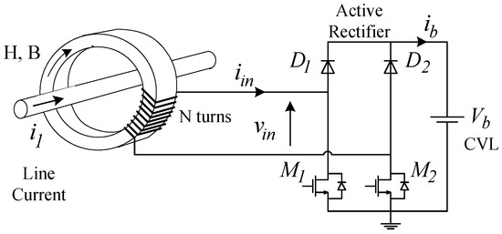
Figure 1.
Overhead line magnetic energy harvester with an active rectifier feeding a constant voltage load.
The circuit in Figure 1 was investigated in the recent literature [19,20,21,22], which suggests several approaches to deal with the challenging problem of core nonlinearity. For instance, its earlier counterpart [19] applied a cot(*) function to accurately model core nonlinearity. Yet, due to the complex nature of such an approximating function, after a few theoretical steps, the final solutions were obtained only numerically.
This article aims to develop an approximated, yet complete, nonlinear analytical model and solution for an overhead line magnetic energy harvester with an active rectifier (OLMEH-AR), under a constant voltage load, as shown in Figure 1.
The proposed model is derived by applying piecewise nonlinear analysis, relying on the Froelich equation to model the B-H characteristics of the magnetic core. The Froelich approximation is based on a first-order rational function. The advantage of the offered approach is that it lends itself to the analytical treatise. The result is a complete closed-form analytical solution to the problem that is quite accurate, simple, and suited for engineering applications.
The rest of the paper is as follows: simulated waveforms, state analysis, and derivation of equivalent circuits are given in Section 2; also, this section presents the analytical model of the OLMEH-AR and derives the expressions for the power transfer window, output current, and the output power and the conditions for maximum power. Experimental measurements of a laboratory prototype are reported in Section 3 and stand in good agreement with the proposed theoretical predictions.
2. The Applied Methodology
2.1. State Analysis and Equivalent Circuits
Analysis of the OLMEH-AR started with computer simulation (PSIM v. 9.1). Derivation of the computer model of the magnetic core in PSIM v9.1 software is a tedious trial-and-error process; however, the computer simulation model proved to be an indispensable tool in the undertaken study.
Examination of the simulated waveforms of the OLMEH-AR in Figure 2 reveals that its operation period comprises two symmetrical half cycles. The positive half-cycle commences when the secondary current becomes positive, i2(t) > 0 and comprises four states. Note that during the negative half-cycle, a similar order of events occurs (with M2 interchanging its function with M1 and D2 interchanging its function with D1). Therefore, it is sufficient to analyze only the positive half-cycle.
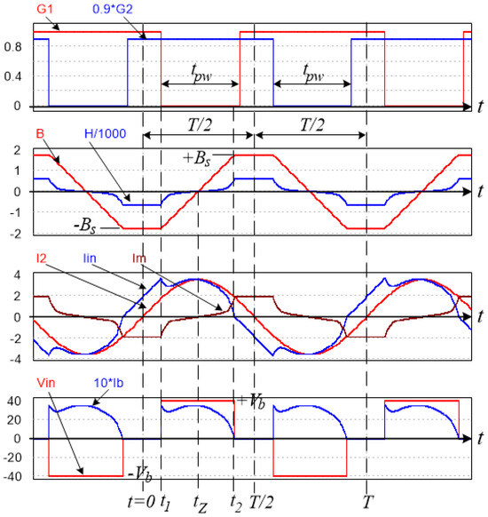
Figure 2.
Typical simulated waveforms of an OLMEH-AR under CVL.
State 1 [0, t1], see Figure 3a, commences at t = 0. Here, both active switches conduct and effectively short the secondary winding.
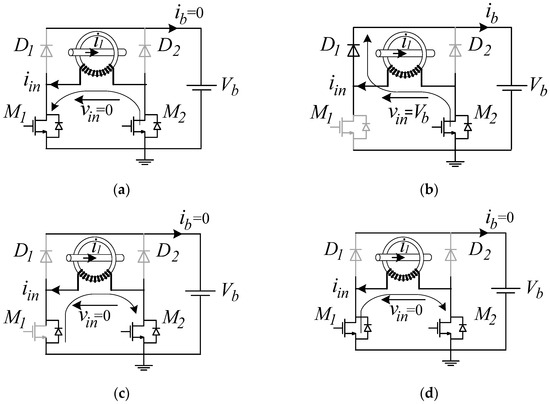
Figure 3.
Semiconductor conduction states during State 1 (a); State 2 (b); State 3 (c); and State 4 (d).
State 2 [t1, t2], see Figure 3b, commences at t = t1, when, by the controller’s command, the M1 switch is turned off but M2 remains on. Here, the rectifier diode D1 turns on and allows the current to charge the battery. Since a constant battery voltage is applied to the secondary winding, the flux density in the core starts ramping up linearly, while causing the magnetizing current to rise in a nonlinear fashion.
State 3 [t2, t1 + tpw], see Figure 3c, commences at t = t2 when the rectifier currents drop to zero, iin = ib = 0. Here, the anti-parallel diode of the M1 switch starts conducting and shorts the secondary winding.
State 4 [t1 + tpw, T/2], see Figure 3d, commences when, by the controller’s command, switch M1 is turned on again and helps its anti-parallel diode to keep the winding shorted. Under short circuit conditions, the flux density in the core remains constant until the end of the positive half cycle.
The OLMEH-AR model based on a simplified cantilever model with a saturable magnetizing inductance, Lm, placed on the secondary winding, while neglecting the leakage inductance, is shown in Figure 4a. The ideal transformer acknowledges the fact that the line conductor acts as a single-turn primary winding, while the secondary one consists of the turn wound on the OLMEH’s core. The simplified equivalent circuit of the short-circuit (SC) state (States 1, 3, and 4) is shown in Figure 4b, and the simplified model of State 2, the only charging state (CS) that allows current to the load, is presented in Figure 4c.
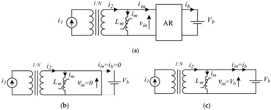
Figure 4.
General model of the overhead line magnetic energy harvester with an active rectifier (OLMEH-AR) with a constant voltage load (a); its equivalent short circuit States 1, 3, and 4 (b) and the equivalent charging State 2 (c).
2.2. The Froelich Equation Review
To facilitate the analysis approach, the following simplifying assumptions are adopted.
Firstly, ideal (lossless) rectifiers and ideal switches are assumed with no voltage drop and zero ON resistance. Secondly, the core is assumed to be un-hysteretic (lossless), whose nonlinearity can be described by the Froelich equation:
Here, the parameter is the saturation flux density at infinite field intensity:
whereas is related to the magnetic permeability of the core at the low field intensity (linear) region
2.3. Analysis: Power Transfer Window
The following definitions are introduced: is the number of OLMEH secondary turns, is the line (primary) current amplitude, and is the amplitude of the secondary current. As usual, is the line frequency.
Examining the waveforms in Figure 2 reveals that the magnetic flux density swings from its initial negative saturation value towards the positive saturation value . The transition is linear since it results from the application of the constant voltage to the secondary winding; see Figure 3b and Figure 4c. Therefore
whence
The practical saturation level that the core can reach, , is presumed to be lower than the heavy saturation flux density level, , defined by (2).
The time interval that appears in (5)
is defined as the power transfer window. To allow the charging current pulse to terminate naturally, the pulse width, tpw, set by the controller, see Figure 2, has to be appropriately matched so that . Switching the MOSFET on, see Figure 3d, decreases the resistance of the conductive path, minimizes the conduction losses during the SC states, and so increases the OLMEH’s conversion efficiency.
Combining (5) with the Froelich Equation (1) yields the magnetic field intensity attained by the core at the peak of saturation:
The right-hand side of (7) was attained by Ampere’s law.
Further examination of the waveforms in Figure 2 suggests that charging State 2 is terminated when the magnetizing current equals the secondary current:
Hence, substituting (8) into (7) yields
Since is set by the controller and assumed to be known, (9) is an equation of a single variable . Yet, (9) is difficult to solve. A straightforward approach to obtain the solution of (9) is to proceed with numerical analysis. An alternative approach offered here is obtaining an analytical solution through approximation of the sine function on the right-hand side of (9) by a rational function, considering that the range of interest lies somewhere in . As a compromise between complexity and accuracy, it is suggested to approximate the falling segment of the sine function using
With K1 = 3.232 and K2 = 6.003, (10) agrees with the function at 120°, 150°, and 180°, thus providing good accuracy within the range of interest. A comparison plot of the function to the chosen approximation function (10) is shown in Figure 5.
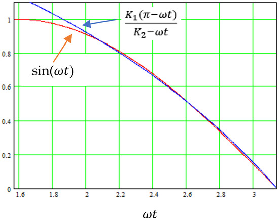
Figure 5.
Comparison plot of the sin() function to the chosen approximation function (10) (for K1 = 3.232 and K2 = 6.003).
Substitution of (10) into (9) yields
Introducing the definitions of the normalized time
the normalized secondary current
the normalized load voltage
and applying (12)–(14) to (11) yields the normalized equation:
which, after some manipulation, can be written in the form of a standard quadratic equation:
where the coefficients are
Only the solution for (i.e., ) has a physical meaning, therefore:
Translating (20) from the normalized time to the real-time, see (12), gives the termination instant of charging State 2:
Since the firing instant is set by the controller and is known and the extinction instant can be obtained from (21), the power transfer window can be found by (6). This allows for the calculation of the output power of the OLMEH-AR as shown next.
2.4. Analysis: Output Current and Power
The rectifier’s input current is the difference between the secondary current, , and the magnetizing current, ; see Figure 4c. Therefore, the charge delivered to the CVL during a half cycle is
Examining the waveforms in Figure 2 reveals that in the steady-state, the magnetizing current is symmetrical. This means that the charge drawn by the magnetizing current is zero:
This also complies with the principle that for the lossless system in the steady state, the energy captured by an ideal magnetizing inductance is fully recycled.
Combining (22) and (23), the average output current can be found as:
whence the average output power delivered to the constant voltage load is
2.5. Analysis: Maximum Power Conditions
Recall again that the delay time, , in (25) is an independent variable set by the controller’s command, whereas , given by (20), (21) is a function of as well as the OLMEH’s parameters and operation conditions. Thus, the question arises regarding the proper choice of the delay time to optimize/maximize the OLMEH’s power output. Symmetry considerations, see Appendix A for details, suggest that the maximum output power can be attained when the power transfer window is aligned symmetrically to the line current peak:
Substituting (26) into (25), the maximum power that can be obtained from the OLMEH-AR under the MPP condition is
Whereas the optimum delay time, , required to implement the MPP condition is found by normalizing the condition (26) and substituting it into (15). Further manipulation of the expression leads to the following quadratic equation:
where
Only the positive solution for has a physical meaning:
Translating the normalized time (32) to the real-time yields:
The results of (32), and (33) allow for optimally locating the power transfer window for optimal energy harvesting; see (27).
3. Comparison with the Experimental Results
An experimental laboratory OLMEH prototype, as shown in Figure 1, and its power processing unit were built and tested. The OLMEH’s core was constructed by stacking together three pairs of 10H10 C-cores made of silicon steel (EILOR MAGNETIC CORES). The magnetic path length was lc = 120 mm, and the total core cross-section of Ac = 1800 mm2. The total number of secondary turns was N = 40.
NTP011N115MC MOSFETs and Schottky rectifiers STP80H100TV were used. The prototype controller was developed and built to allow for adjustment of the delay time, t1, and the controller’s power transfer window width, tpw, independently.
The Froelich parameters of the core a and b were established by curve fitting to the experimental data. Measured B-H characteristics of a silicon steel core sample vs. the fitted BH curve, drawn by using the extracted Froelich parameters, are shown in Figure 6. Here, a = 2.05 [T] and b = 109.4 [At/m] were found, the same as in [10].
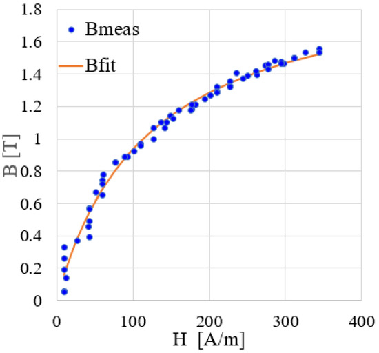
Figure 6.
Comparison of the measured BH curve of the silicon steel core sample (EILOR MAGNETIC CORES) to its Froelich approximation [10].
Typical waveforms of the experimental OLMEH with an active rectifier at line current I1 = 100 A rms under constant voltage load, Vb = 45 V, are shown in Figure 7. Here, the waveforms shown are: line current i1(t), the rectifier input current iin(t), and the gating signal of the M1 switch, vg(t), generated by the controller. The math channel shows the instantaneous output power po(t). Recall that energy transfer to the CVL occurs during the high level of the v1(t) waveform. Note that the primary voltage, v1(t), was measured across the line conductor segment of only about 10 cm long. Also, it is worth noting that (during the positive half cycle), the saturation of the core manifests itself by the rapidly falling edge of the iin(t) current. The energy stored by the magnetizing inductor manifests itself by the offset segment seen in the iin(t) waveform, when the v1(t) is at its zero level. The release of the stored energy is manifested by the down-going step in the iin(t) waveform.
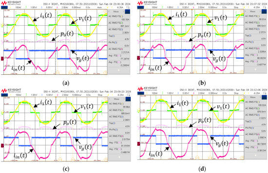
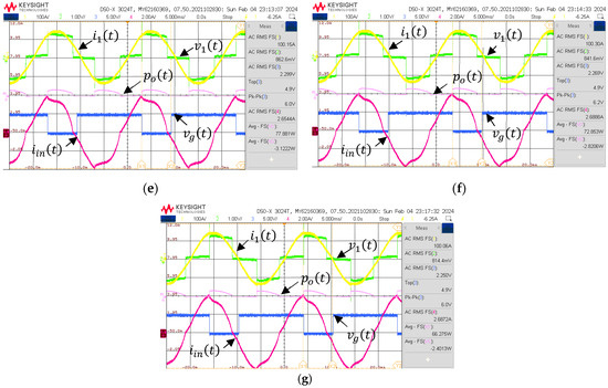
Figure 7.
Typical waveforms of the experimental OLMEH with an active rectifier at line current I1 = 100 A rms: Vb = 45 V. Delay time: (a) t1 = 1 mS; (b) t1 = 1.5 mS; (c) t1 = 2 mS; (d) t1 = 2.5 mS; (e) t1 = 3 mS; (f) t1 = 3.5 mS; (g) t1 = 4 mS.
The theoretical derivations were first verified by simulation. Figure 8 shows the comparison of the calculated vs. the simulated results for the output power. Here, the assumed line current was Iline = 100 A rms and Iline = 200 A rms (also N = 40, Vb = 45 V). Good agreement between the results was found.
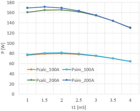
Figure 8.
Comparison of the simulated vs. calculated OLMEH’s output power as a function of the delay time, , for line current of Iline = 100 A rms and Iline = 200 A rms, (here, N = 40 and Vb = 45 V).
Comparison of the experimentally measured vs. calculated by (33) and (27) output power as a function of the delay time t1, for line current Iline = 100 A rms and constant load voltage Vb = 45 V, as shown in Figure 9. A good match between the experimental and theoretically predicted power can be observed.
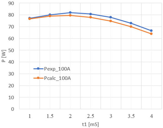
Figure 9.
Comparison of the experimentally measured vs. calculated output power as a function of the delay time . (For Iline = 100 A rms; Vb = 45 V).
The experimental work revealed that handling the OLMEH prototype brought about variations in its magnetic properties, primarily due to variations in the technological air gap between the two halves of the C-core, which depend on factors like mounting force and surface imperfections. Therefore, some inaccuracies can be seen in the presented comparison plots.
The view of the experimental prototype OLMEH and its test bench are shown in Figure 10a and Figure 10b, respectively, and they are similar to that used in [10].
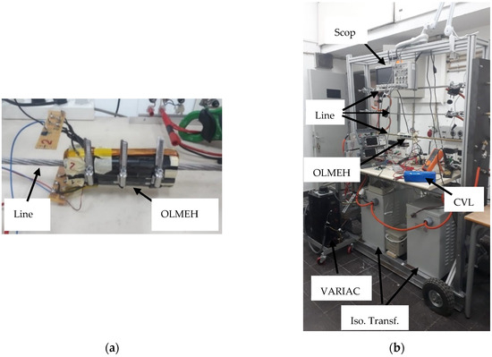
Figure 10.
View of the experimental prototype OLMEH (a) and its test bench (b) [10].
4. Conclusions
This paper aims to offer a closed-form solution for an overhead line magnetic energy harvester with an active rectifier (OLMEH-AR) operating under a constant voltage load.
The article initially examines the Froelich equation, which is subsequently utilized as a fundamental instrument to scrutinize the OLMEH-AR’s functionality. The selection of the Froelich equation as the approximation function to characterize the core BH curve is crucial and has been demonstrated to be well suited for facilitating the derivation of a comprehensive analytical model of an OLMEH-AR. The offered model allowed for an extensive analytical study of the OLMEH-AR which yielded approximate analytical solutions for charging and idle periods, the power transfer window, the mean output current, and the mean output power.
An important note drawn from the experimental work is that manipulating the OLMEH-AR prototype affects the magnetic core parameters. This is primarily due to variations in the technological air gap remaining between the two halves of the C-core, which depend on factors such as misalignment, mounting force, and surface imperfections. Therefore, the authors believe that developing a more precise and complex theoretical model, including hysteresis effects, temperature effects, etc., is of limited practical value because of the unavoidable core parameter variations.
As compared to the passive rectifier case, the application of an active rectifier significantly increases the harvester’s output power [10]. This comes as a result of two key features, which the passive rectifier does not possess. First is that the controlled rectifier allows for the storage of magnetic energy by short-circuiting the OLMEH’s secondary winding, and, secondly, the active rectifier allows aligning the power transfer window to track the optimal power point. The output characteristics of the OLMEH and its proper matching, considering variable line current and load voltage conditions, have also been reported in recent papers [23,24,25].
While the advantage of the uncontrolled rectifier is its simplicity and robustness, the advantages of the active rectifier are the ability to control the CVL charging current as well as providing overcharge and line overcurrent protection features. However, realizing the active rectifier functions requires a somewhat sophisticated approach, synchronized to the line current control circuit.
Author Contributions
Conceptualization, A.K.; methodology, A.A.; software, A.A.; validation, A.A. and M.S.; formal analysis, A.A.; investigation, A.A.; resources, A.K.; data curation, M.S.; writing—original draft preparation, A.A.; writing—review and editing, A.A.; visualization, A.A. and M.S.; supervision, A.K.; project administration, A.K.; funding acquisition, A.K. All authors have read and agreed to the published version of the manuscript.
Funding
This research received no external funding.
Institutional Review Board Statement
Not applicable.
Informed Consent Statement
Not applicable.
Data Availability Statement
The original contributions presented in the study are included in the articl, further inquiries can be directed to the corresponding author.
Conflicts of Interest
The authors declare no conflicts of interest.
Nomenclature
Throughout this paper, the following definitions of key parameters were adopted.
| Time (continuous) | t |
| State 1 termination instant | t1 |
| State 2 termination instant | t2 |
| Flux density zero crossing instant | tZ |
| Power line angular frequency | |
| Flux density | |
| Saturation flux density | Bs |
| Field intensity | |
| Saturation field intensity | Hs |
| Froelich coefficients | a, b |
| Number of turns | N |
| Magnetic path length | lc |
| Magnetic core area | Ac |
| Line (primary) current instantaneous | i1(t) |
| Line (primary) current amplitude | I1m |
| Secondary current instantaneous | i2(t) |
| Secondary current amplitude | I2m |
| Magnetizing current, (instantaneous) | im(t) |
| Rectifiers’ input (AC side) voltage | |
| Rectifiers’ input (AC side) current | |
| CVL voltage | Vb |
| CVL current | |
| Average output power | Po |
Appendix A
In our case, the delay angle is and the extinction angle is . We found the condition on maximizing the function .
Applying the classical extremum finding procedure:
whence
Comparison of the argument on the left hand-side and the right hand-side yields the delay angle:
whence the extinction angle is
Hence, to attain the MPP condition, the pulse edges should be aligned symmetrically relative to ; thus, (26) follows.
References
- Kang, S.; Yang, S.; Kim, H. Non-intrusive voltage measurement of ac power lines for smart grid system based on electric field energy harvesting. Electron. Lett. 2017, 53, 181–183. [Google Scholar] [CrossRef]
- Moghe, R.; Lambert, F.C.; Divan, D. Smart “stick-on” sensors for the smart grid. IEEE Trans. Smart Grid 2012, 3, 241–252. [Google Scholar] [CrossRef]
- Moghe, R.; Iyer, A.R.; Lambert, F.C.; Divan, D.M. A low-cost wireless voltage sensor for monitoring MV/HV utility assets. IEEE Trans. Smart Grid 2014, 5, 2002–2009. [Google Scholar] [CrossRef]
- Gu, I.Y.H.; Sistiaga, U.; Berlijn, S.M.; Fahlstrom, A. Online detection of snow coverage and swing angles of electrical insulators on power transmission lines using videos. In Proceedings of the 16th IEEE International Conference on Image Processing (ICIP 2009), Cairo, Egypt, 7–10 November 2009; pp. 3249–3252. [Google Scholar] [CrossRef]
- Zhong, Y.-P.; Zuo, Q.; Zhou, Y.; Zhang, C. A new image-based algorithm for icing detection and icing thickness estimation for transmission lines. In Proceedings of the IEEE International Conference on Multimedia and Expo Workshops (ICMEW), San Jose, CA, USA, 15–19 July 2013; pp. 1–6. [Google Scholar] [CrossRef]
- Riba, J.-R.; Moreno-Eguilaz, M.; Bogarra, S. Energy Harvesting Methods for Transmission Lines: A Comprehensive Review. Appl. Sci. 2022, 12, 10699. [Google Scholar] [CrossRef]
- Moon, J.; Leeb, S.B. Power Electronic Circuits for Magnetic Energy Harvesters. IEEE Trans. Power Electron. 2016, 31, 270–279. [Google Scholar] [CrossRef]
- Enayati, J.; Asef, P. Review and Analysis of Magnetic Energy Harvesters: A Case Study for Vehicular Applications. IEEE Access 2022, 10, 79444–79457. [Google Scholar] [CrossRef]
- Deng, Z.; Dapino, M.J. Review of magnetostrictive vibration energy harvesters. Smart Mater. Struct. 2017, 26, 103001. [Google Scholar] [CrossRef]
- Abramovitz, A.; Shwartsas, M.; Kuperman, A. Nonlinear Analysis and Closed-Form Solution for Overhead Line Magnetic Energy Harvester Behavior. Appl. Sci. 2024, 14, 9146. [Google Scholar] [CrossRef]
- Moon, J.; Leeb, S.B. Wireless sensors for electromechanical system diagnostics. IEEE Trans. Instr. Meas. 2018, 67, 2235–2246. [Google Scholar] [CrossRef]
- Liu, Z.; Li, Y.; Duan, N.; He, Z. An energy management method for magnetic field energy harvesters under wide-range current in railway electrification systems. IEEE Trans. Ind. Electron. 2024, 71, 5360–5369. [Google Scholar] [CrossRef]
- Monagle, D.; Ponce, E.A.; Leeb, S.B. Rule the Joule: An energy management design guide for self-powered sensors. IEEE Sens. J. 2024, 24, 6–15. [Google Scholar] [CrossRef]
- Suntio, T.; Viinamaki, J.; Jokipii, J.; Messo, T.; Kuperman, A. Dynamic characterization of power electronic interfaces. IEEE J. Emerg. Sel. Top. Power Electron. 2014, 2, 949–961. [Google Scholar] [CrossRef]
- Monagle, D.; Ponce, E.; Leeb, S.B. Generalized analysis method for magnetic energy harvesters. IEEE Trans. Power Electron. 2022, 37, 15764–15773. [Google Scholar] [CrossRef]
- Li, Y.; Duan, N.; Liu, Z.; Hu, J.; He, Z. Impedance-matching-based maximum power tracking for magnetic field energy harvesters using active rectifiers. IEEE Trans. Ind. Electron. 2023, 70, 10730–10739. [Google Scholar] [CrossRef]
- Chen, F.; Yang, C.; Guo, Z.; Wang, Y.; Ma, X. A magnetically controlled current transformer for stable energy harvesting. IEEE Trans. Power Deliv. 2023, 38, 212–221. [Google Scholar] [CrossRef]
- Kuperman, A.; Averbukh, M.; Lineykin, S. Maximum power point matching versus maximum power point tracking for solar generators. Renew. Sustain. Energy Rev. 2013, 19, 11–17. [Google Scholar] [CrossRef]
- Moon, J.; Leeb, S.B. Analysis Model for Magnetic Energy Harvesters. IEEE Trans. Power Electron. 2015, 30, 4302–4311. [Google Scholar] [CrossRef]
- Gao, M.; Yi, L.; Moon, J. Mathematical modeling and validation of saturating and clampable cascaded magnetics for magnetic energy harvesting. IEEE Trans. Power Electron. 2023, 38, 3455–3468. [Google Scholar] [CrossRef]
- Vos, M.J. A magnetic core permeance model for inductive power harvesting. IEEE Trans. Power Electron. 2020, 35, 3627–3635. [Google Scholar] [CrossRef]
- Liu, Z.; Li, Y.; Yang, H.; Duan, N.; He, Z. An accurate model of magnetic energy harvester in the saturated region for harvesting maximum power: Analysis, design and experimental verification. IEEE Trans. Ind. Electron. 2023, 70, 276–285. [Google Scholar] [CrossRef]
- Abramovitz, A.; Shvartsas, M.; Orfanoudakis, G.I.; Kuperman, A. Output Characteristics of Passive Magnetic Energy Harvester Feeding a Constant-Voltage-Type Load. IEEE J. Emerg. Sel. Top. Power Electron. 2024, in press. [Google Scholar] [CrossRef]
- Abramovitz, A.; Shvartsas, M.; Kuperman, A. Enhanced Maximum Power Point Reaching Method for Passive Magnetic Energy Harvesters Operating Under Low Primary Currents. IEEE Trans. Power Electron. 2024, 39, 6619–6623. [Google Scholar] [CrossRef]
- Abramovitz, A.; Shvartsas, M.; Kuperman, A. On the Maximum Power of Passive Magnetic Energy Harvesters Feeding Constant Voltage Loads Under High Primary Currents. IEEE Trans. Power Electron. 2024, 39, 12076–12080. [Google Scholar] [CrossRef]
Disclaimer/Publisher’s Note: The statements, opinions and data contained in all publications are solely those of the individual author(s) and contributor(s) and not of MDPI and/or the editor(s). MDPI and/or the editor(s) disclaim responsibility for any injury to people or property resulting from any ideas, methods, instructions or products referred to in the content. |
© 2024 by the authors. Licensee MDPI, Basel, Switzerland. This article is an open access article distributed under the terms and conditions of the Creative Commons Attribution (CC BY) license (https://creativecommons.org/licenses/by/4.0/).