Bias and Variance Analysis of Contemporary Symbolic Regression Methods

Featured Application

Scientific machine learning, white box modelling.

Abstract

Symbolic regression is commonly used in domains where both high accuracy and interpretability of models is required. While symbolic regression is capable to produce highly accurate models, small changes in the training data might cause highly dissimilar solution. The implications in practice are huge, as interpretability as key-selling feature degrades when minor changes in data cause substantially different behavior of models. We analyse those perturbations caused by changes in training data for ten contemporary symbolic regression algorithms. We analyse existing machine learning models from the SRBench benchmark suite, a benchmark that compares the accuracy of several symbolic regression algorithms. We measure the bias and variance of algorithms and show how algorithms like Operon and GP-GOMEA return highly accurate models with similar behavior despite changes in training data. Our results highlight that larger model sizes do not imply different behavior when training data change. On the contrary, larger models effectively prevent systematic errors. We also show how other algorithms like ITEA or AIFeynman with the declared goal of producing consistent results meet up to their expectation of small and similar models.

1. Introduction

Symbolic regression (SR) is a task where we aim to find a closed-form mathematical equation which describes linear and nonlinear dependencies in data without making prior assumptions. The goal is to make predictions for unseen data by training a mathematical expression with a finite set of existing observations. While there is a huge variety of methods for solving regression problems, starting from linear models over decision trees [1] up to neural networks [2], SR methods deliver non-linear and human-readable closed-form expressions as models with smooth and differentiable outputs. Therefore, SR is commonly applied in situations where we cannot rely on black-box models like neural networks, as they require comprehensible and traceable results for throughout model verification.

Bias and variance are properties of a machine learning algorithm that affect the interpretability of its models. The variance of an algorithm describes, how the outputs of its models change when there are differences in the used training data. SR algorithms are considered as high-variance algorithms, which means that even slightly different training data can lead to very dissimilar models [3]. However, high variance of an algorithm implies that it is capable to fit a model, to a certain extent, perfectly to training data. It is often necessary to limit the variance in order to perform well on unseen data, without restricting it too much, which would prevent highly accurate models and cause so-called bias. Balancing both properties is called the bias/variance trade-off [1].

From a practitioner’s point of view, perturbations caused by variance do not spark trustworthiness for practitioners, as we would expect small changes in training data to have little effect on the overall results. Therefore, many algorithms use, e.g., statistical tools to gracefully deal with bias and variance or ignore this property as the primary focus is accuracy regardless of the model structure [4]. However, bias and variance have specific implications to SR. SR is known for its human-readable and potentially interpretable white-box model structure, but high variance limits this feature. On the other hand, the complexity of models is limited for the sake of interpretability, which causes bias. Algorithmic aspects of SR amplify these effects: First, the stochastic nature of a Genetic Programming (GP)-based [5] SR algorithm results in differences in models between multiple SR runs even when the training data do not change at all. Second, since there is no guarantee for optimality in an SR search space [6], models trained in different SR runs might even provide very similar accuracy despite being completely different mathematical expressions due to, e.g., bloat [5] or over-parameterization [7] that increase the size of a model without affecting its accuracy.

1.1. Research Question

Controlling the variance while still achieving high accuracy is an ambient goal in SR research and both directly and indirectly targeted by new algorithms. In this work, we examine the bias and the variance of contemporary SR algorithms. We show which algorithms perform most consistent despite perturbations in training data. The results are put into perspective with their achieved accuracy and parsimony. We analyze which algorithms in recent SR research have been the most promising regarding robustness and reliability by mitigating variance while still providing high accuracy. This work complements and builds upon the existing results of the SRBench benchmark [8], which is a solid benchmark suite for SR algorithms. SRBench compares the accuracy of several SR algorithms for problems from the PMLB benchmark suite [9]. The results, which are available at cavalab.org/srbench (accessed on 21 November 2024), also include the trained models for each algorithm and data set. We reuse these published results and analyze the bias and variance of the already published models.

1.2. Related Work

Although most algorithmic advancements in SR algorithms affect their bias and variance, actual measurements and analyses of these properties are sparse. One analyses of bias and variance of SR algorithms was done by Keijzer and Babovic [10]. They calculated bias and variance measurements but only for few data sets and only for ensemble bagging of standard GP-based SR. Kammerer et al. [11] analyzed the variance for two different GP-based SR variants and compared them with Random Forest regression [12] and linear regression on few data sets. Highly related to bias and variance is the work by de Franca et al. [13], who provided a successor of SRBench. In this benchmark, they tested specific properties of algorithms for a few specific data sets, instead of only the accuracy and model size for a wide range of different data sets. Those tests included, e.g., whether algorithms identified the ground truth on a symbolic level instead of just approximating it with an expression of any structure. In our work, we use the first version of SRBench as we focus on the semantic of models on a broad range of data sets. More research about bias and variance was performed on other algorithms, most recently for neural networks by Neal et al. [4] and Yang et al. [14]. They evaluated the relation between bias/variance to model structure and number of model parameters. Belkin et al. [15] questioned the classical understanding of the relationship between bias and variance and their dependence on the dimensionality of the problem for very large black-box models.

2. Bias/Variance Decomposition

In supervised machine learning tasks, we want to identify a function $\widehat{f}\left(x\right)=y$, which approximates the unknown ground truth $f\left(x\right)$ for any x drawn from a problem-specific distribution P. x is a vector of so-called features and y the scalar target. The target values contain randomly distributed noise $ϵ$. In this work, we define $ϵ\sim \mathrm{N}(0,\sigma )$ with $\sigma$ being a problem-specific standard deviation, as it is done in SRBench [8]. Therefore, our data-generating function is $y=f\left(x\right)+ϵ$. To find an approximation $\widehat{f}\left(x\right)$, we use a training set $D=\{(x_1,y_1),\dots ,(x_n,y_n)\}$ with $x_i\sim P$ and their corresponding y values. The goal of machine learning is to learn a prediction model $\widehat{y}=\widehat{f}(x,D)$ which minimizes a predefined loss function $L(y,\widehat{y})$ on a training set D. This means that the output of a machine learning model depends on the used algorithm, the features x and the set of training samples D.

Bias and variance of an algorithm occur due to changes in the training data D and have a direct effect on the error and loss of models. We use the mean squared error as the loss function. For this loss function, Hastie et al. [1] describe that a model’s expected error on previously unseen data consists of bias, variance and irreducible noise $ϵ$. However, Domingos [16] describes how the decomposition of the error into bias and variance is also possible for other loss functions.

The distribution of training sets D that contain values drawn from P also leads to a distribution of model outputs $\widehat{y_0}=\widehat{f}(x_0,D)$ for a single fixed feature vector $x_0$. The bias is the difference between the ground truth value $y_0=f\left(x_0\right)$ and the expected value over D over the $\widehat{f}$ of model outputs ${\mathbb{E}}_D\left[\widehat{f}(x_0,D)\right]$, as depicted in Equation (1). The bias describes, how far our estimation is “off” on average from the truth.

$${\mathrm{Bias}}_D(\widehat{f},x)={\mathbb{E}}_D\left[\widehat{f}(x,D)\right]-f\left(x\right)$$

(1)

$${\mathrm{Var}}_D(\widehat{f},x)={\mathbb{E}}_D\left[{\left({\mathbb{E}}_D\left[\widehat{f}(x,D)\right]-\widehat{f}(x,D)\right)}^2\right]$$

(2)

Variance defines, how far the outputs of estimators spread on a specific point $x_0$ when they were trained on different data sets. It is independent of the ground truth. It is defined in Equation (2) as the expected squared difference between the output of models and the average output of those model on a specific point $x_0$. Both properties are not mutually exclusive. However, algorithms with high variance tend to have lower bias and vice versa, so practitioners need to find an algorithm setting that minimizes both properties. This is called the bias-variance trade-off [1].

An example inspired by Geman et al. [17] for high bias, high variance and an optimal trade-off between both is given in Figure 1 and Figure 2, where we want to approximate an oscillating function with polynomial regression. We use polynomial regression as the results nicely translates to SR as its search space is a subset of SR methods with an arithmetic function set. We add normal distributed noise to each target value y, so $y=f\left(x\right)+ϵ$ with $ϵ\sim \mathrm{N}(0,\sigma )$ and $\sigma =0.2$. Each set of samples D consists of ten randomly sampled observations $D=\{x_1,\dots ,x_{10}\}$ with $x_i\sim \mathrm{N}(\pi ,2)$. 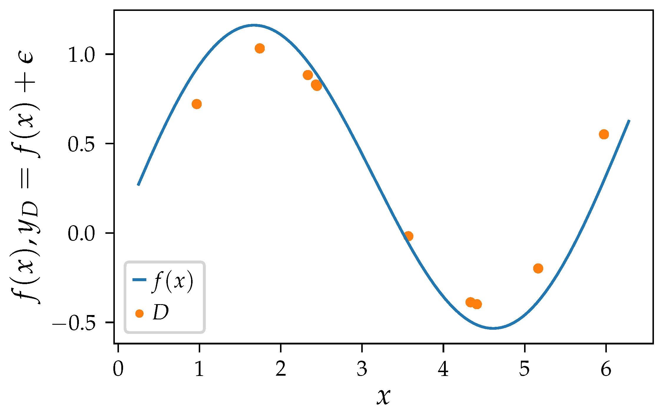Figure 1 shows the ground truth and one training set of samples. We get a different model with every different set of samples D. Depending on the algorithm settings, those models behave more or less similar, resulting in different bias and variance measures. We expect the error of a perfect model to be equally distributed as the irreducible noise $ϵ$.

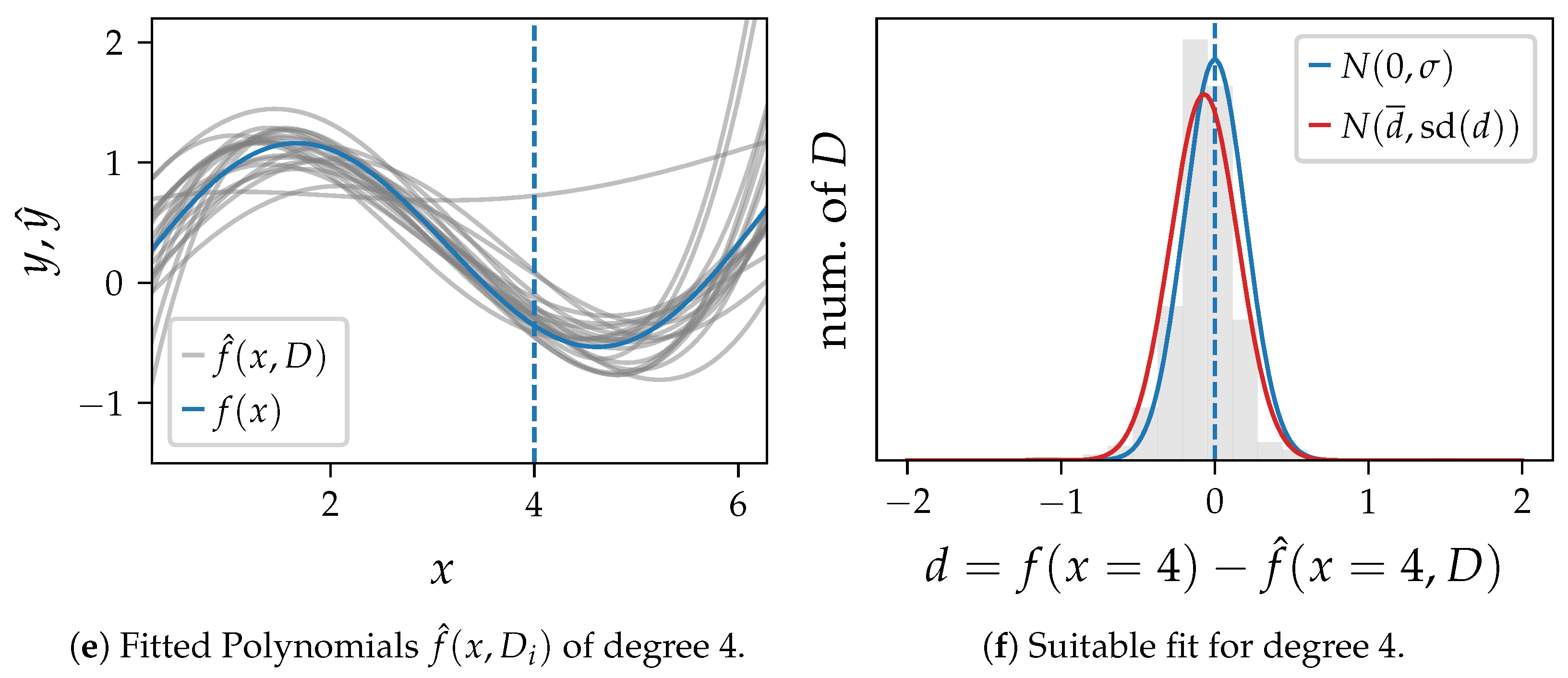
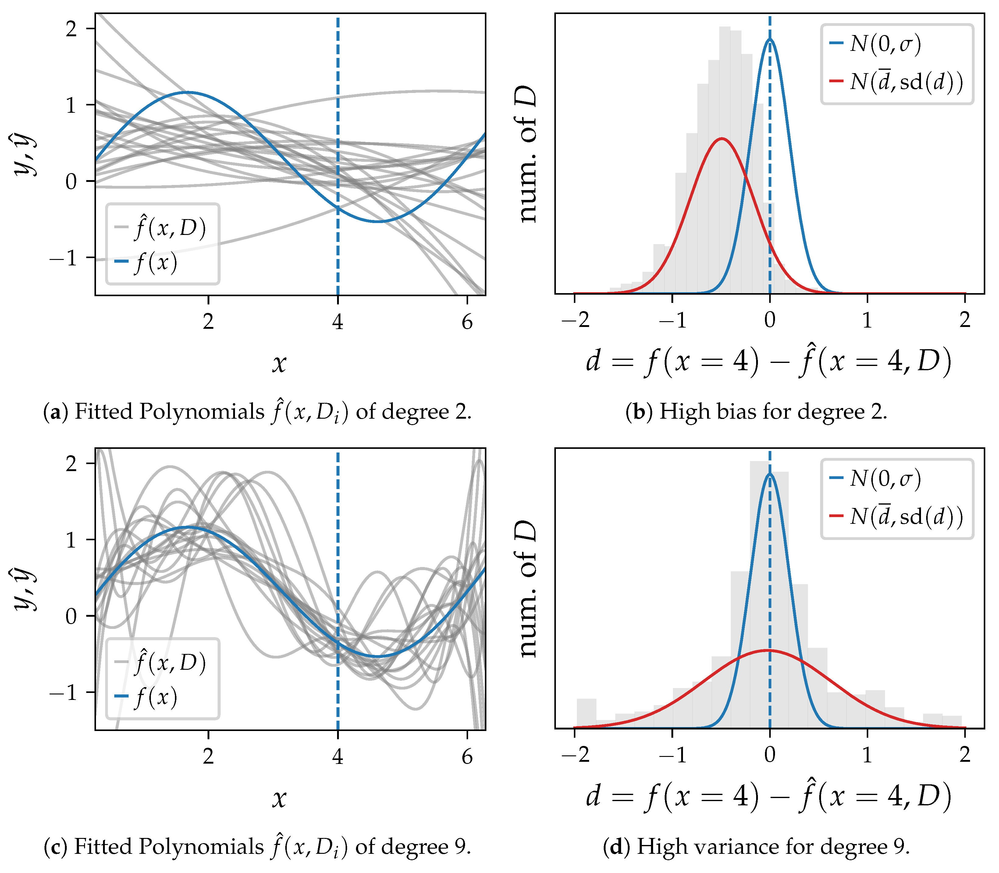
In Figure 2 we draw 1000 sets of samples D and learn one polynomial for each training set for three algorithm settings. 20 exemplary polynomials are shown for each setting in Figure 2a,c,e. The distribution of the difference d between the ground truth and the model output at $x=4$ is shown as histogram in Figure 2b,d,f. These plots also compare the probability density function of $ϵ$ and a normal distribution with the mean and standard deviation ($\mathrm{sd}$) of d as parameters. Figure 2a,b show polynomials of degree 2, which cannot capture oscillations in the data. The variance is high, and the average error $\overline{d}$ clearly differs from the ground truth $f(x=4)$. Figure 2c,d show polynomials of degree 9 with the highest variance and the smallest bias in this example. The error of single predictions at that point is often very high, which makes a single model unusable. However, their average fits the ground truth well, as there is nearly no bias. Figure 2e,f show a polynomial of degree 4, which appears to be an appropriate setting with low bias and variance close to the error variance.

As described before, the bias and variance of an algorithm is directly linked to its model generalization capabilities, as the prediction error on previously unseen data can be decomposed into the square of its bias and its variance [16]. Therefore, we expect algorithms with models that generalize well to be both low in bias and in variance. Of course, not every algorithm is equally capable to produce high quality results, as shown in SRBench. While the error of models is well measured, it is often unclear whether it is primarily caused by variance or bias. As described in Section 1, GP-based algorithms exhibit variance even when there is no change in the training data. On the other hand, deterministic algorithms like FFX and AIFeynman produce equal results on equal inputs. Therefore, we expect more similar models and less variance for those algorithms.

3. Experiments

Our analysis builds upon the data sets and models of the SRBench benchmark [8]. SRBench provides an in-depth analysis of performance and model size of contemporary SR methods on many data sets. The methodology and the results of this benchmark fit perfectly for our purpose, and we can rely on a reviewed setting of algorithms and benchmark data.

SRBench uses the data sets of the PMLB benchmark suite [9,18], the Feynman Symbolic Regression Database [19] and the ODE-Strogatz repository [20]. In total, it contains both real world data and generated data, where the ground truth and noise distribution is known. In this work, we will use SRBench’s results on the 116 datasets from the Feynman Symbolic Regression Database because the ground truth and data distribution is known, so we can arbitrarily generate new data. We refer to those problems as Feynman problems in the following. The Feynman problems are mostly low-dimensional, nonlinear expression that were taken from physics textbooks [21].

In SRBench, four different noise levels $\sigma$ are used for Feynman problems. Given a problem-specific ground truth $f\left(x\right)$, training data y for one problem are generated with $y=f\left(x\right)+ϵ,ϵ\sim \mathrm{N}(0,\sigma )$ and $\sigma \in \{0,0.001,0.01,0.1\}$, with $\mathrm{N}(0,0)$ meaning no noise. This results in 464 combinations of data sets and noise levels. For each of those 464 problems, ten models were trained in the SRBench benchmark per algorithm. A different training set is sampled for each of the ten models [8]. All ten models were trained with the same hyperparameters, which is suitable for our study, because bias and variance are only caused by the search procedure and not by differences in hyperparameters.

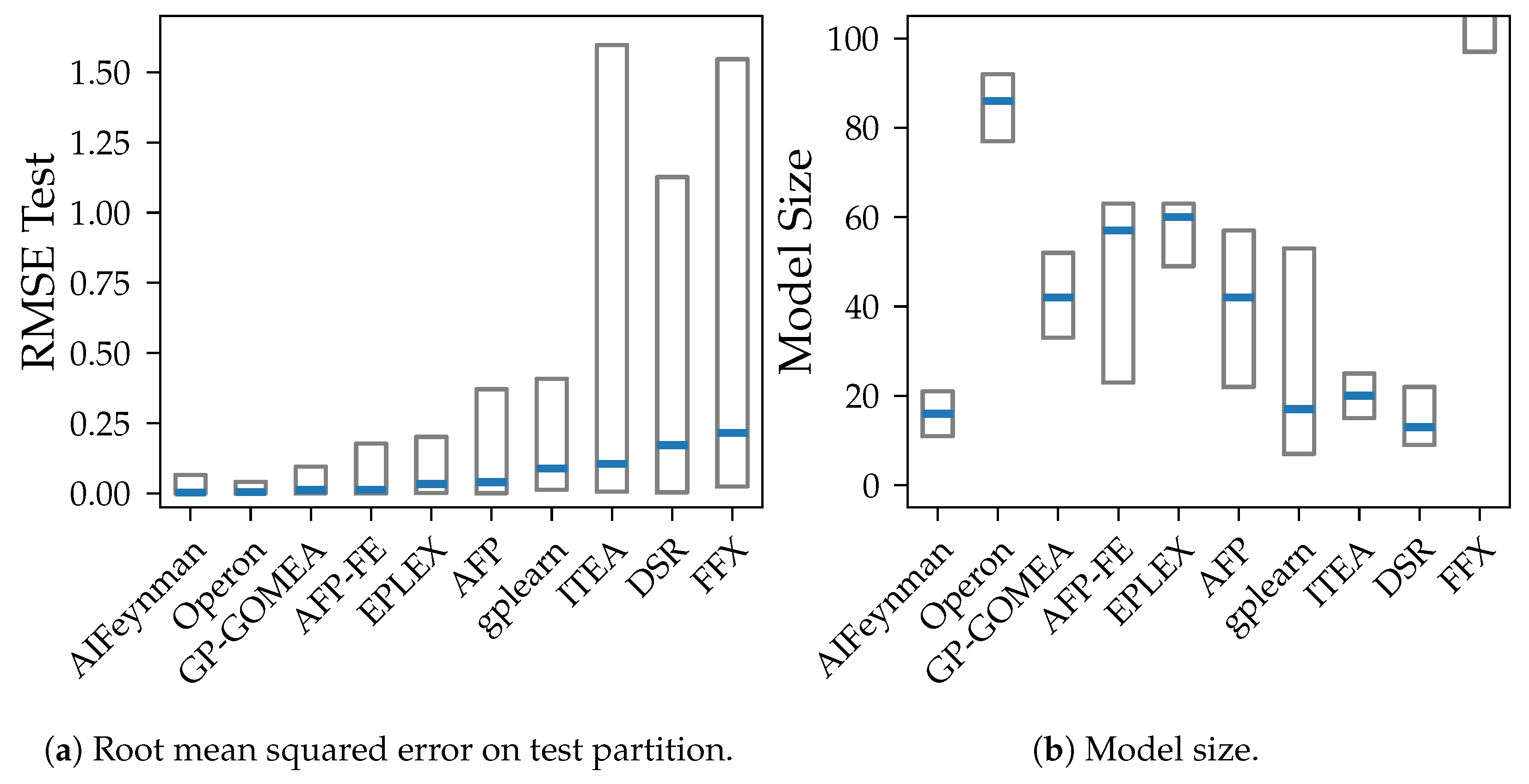
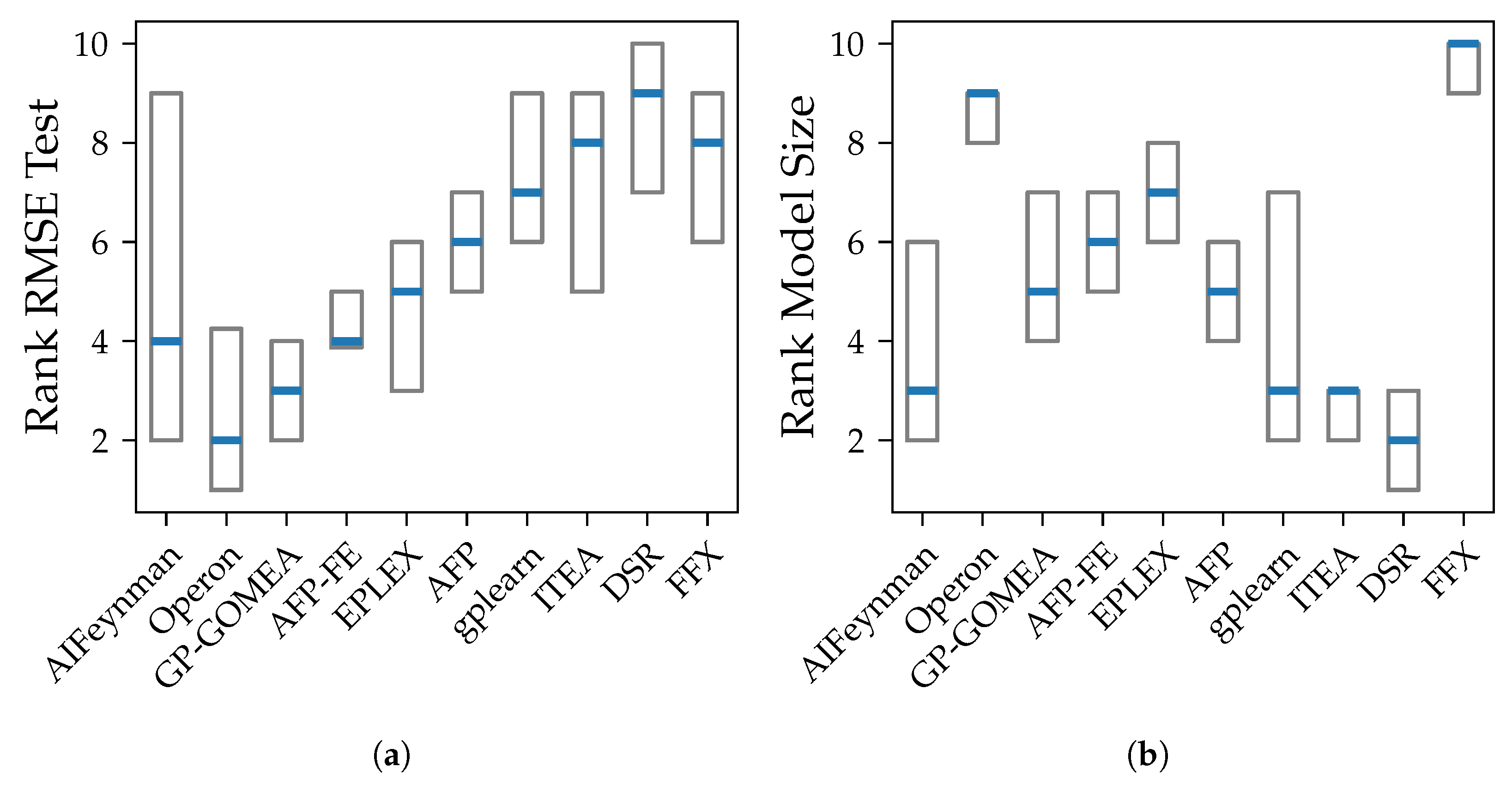
We compare both the accuracy, the model size, bias, and variance. We use the root mean squared error (RMSE) to measure the accuracy, since it is on the same scale as the applied noise and therefore the bias and variance. The model size is the number of symbols in the model as defined in SRBench [13]. The model size describes the inverse of parsimony and is used as a notion of simplicity of a model.

3.1. Bias/Variance Calculation

To compare the bias and variance between problems and algorithms, we use the expected value of the bias and variance over x. Given are a feature value distribution P, a ground truth $f\left(x\right)$, a noise level $\sigma$ with a data generating function $y=f\left(x\right)+ϵ$, $ϵ\sim N(0,\sigma )$ and a distribution of training sets with $D=\{(x_1,y_1),\dots ,(x_m,x_m)\}$, $x_i\sim P$, $m=10,000$. P, $f\left(x\right)$, $\sigma \in \{0,0.001,0.01,0.1\}$ are problem-specific and defined in SRBench.

We reuse the ten models that were trained in SRBench for each problem. Every model was trained on different training set drawn from D. We generate a new set of data $X=\{x_1,\dots ,x_n\},x_i\sim P,n=10,000$ to estimate the expected value for bias and variance for those ten models. We define the estimators as the average of bias and variance over the ten models for all values in X, as defined in Equation (3) for bias and Equation (4) for variance. To prevent sample-specific outliers, we use the one set of samples X per problem for all algorithms.

$$\overline{\mathrm{Bias}}\left(\widehat{f}\right)=\sqrt{{\displaystyle \frac{1}{n}}\sum _{i=1}^n{\mathrm{Bias}}_D{\left(\widehat{f},x_i\right)}^2},x_i\in X$$

(3)

The bias for one value $x_i$ defined in Equation (1) can become both negative and positive. However, we are not interested in the sign of the bias but only in its absolute value. To be consistent with the bias/variance decomposition by Hastie et al. 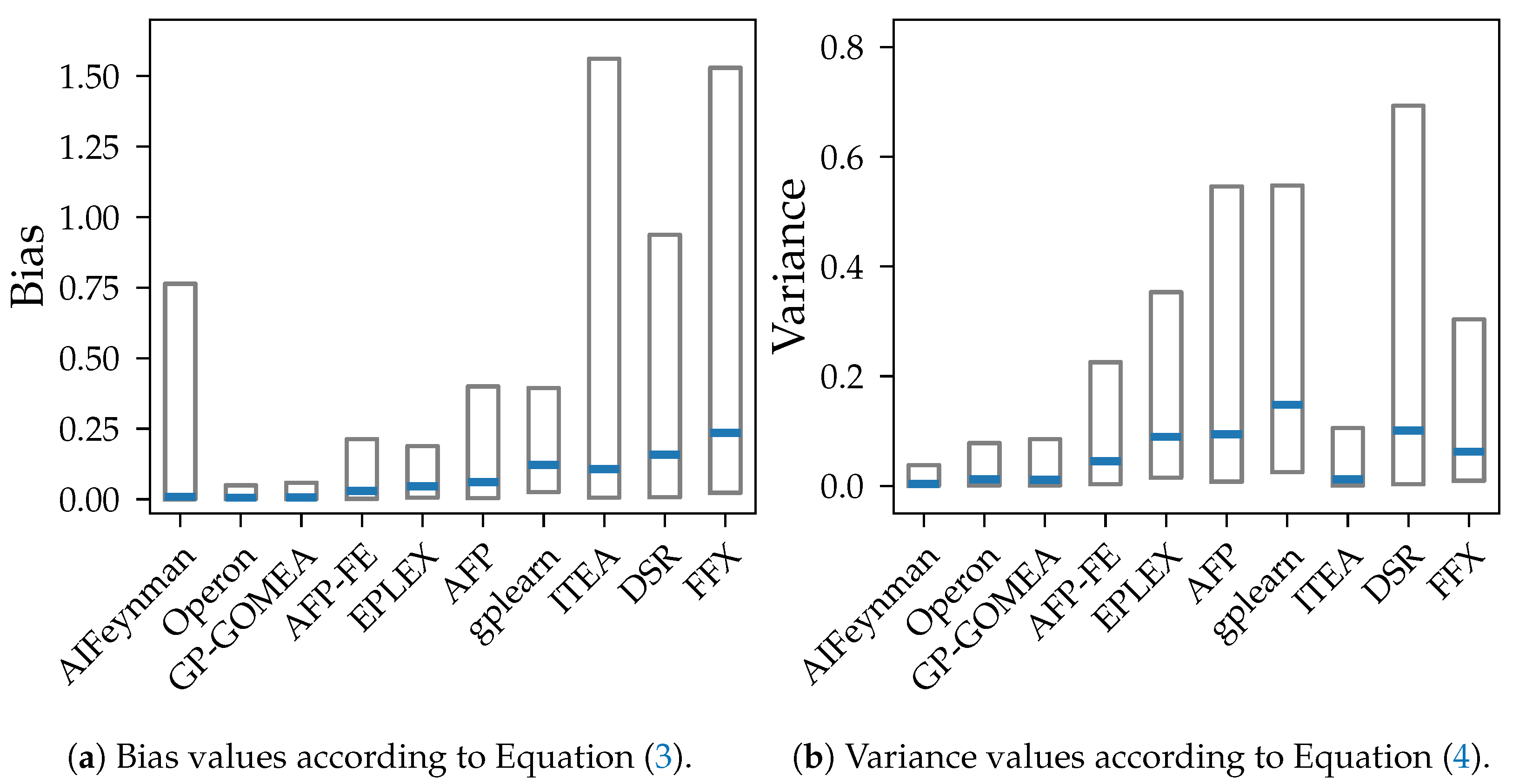[1], which decomposes the error into the sum of variance, the square of bias and an irreducible error, we also use the square of the bias ${\mathrm{Bias}}_D(\widehat{f},x=x_0)$ from Equation (1) for the calculation of bias of the overall problem and algorithm in ${\mathrm{Bias}}_{D,x}\left(\widehat{f}\right)$. We take the square root of the average of the squared bias to be on the same scale as the error of a model.

$$\overline{\mathrm{Var}}\left(\widehat{f}\right)={\displaystyle \frac{1}{n}}\sum _{i=1}^n{\mathrm{Var}}_D\left(\widehat{f},x_i\right),x_i\in X$$

(4)

3.2. SRBench Algorithms and Models

The SR algorithms tested in SRBench provide different approaches to limit the size and/or structure of their produced models to counteract over-fitting and therefore reduce the algorithm’s variance. Therefore, we expect clear differences. E.g., GP implementations such as GP-GOMEA [22], Operon [23], AFP [24] and AFP-FE [25] adapt their search procedure. GP-GOMEA identifies building blocks that cover essential dependencies. Operon, AFP and AFP-FE use a multi-objective search procedure to incorporate both accuracy and parsimony in their objective function [23,24,25]. EPLEX, AFP and AFP-FE use the $ϵ$-lexicase selection in their GP procedure [26], in which instead of one aggregated error value multiple tests are performed over different regions of the training data. ITEA [27] deliberately restricts the structure of their models. gplearn (gplearn.readthedocs.io, accessed on 21 November 2024) provides a GP implementation that is close to the very first ideas about GP-based SR by Koza [5]. DSR [28] is a non-GP-based algorithm that considers SR as a reinforcement learning problem and uses a neural network, another high-variance method, to produce a distribution of small symbolic models. FFX [29] and AIFeynman 2.0 [19] do also not build upon GP but run deterministic search strategies in restricted search spaces. We expect that both determinism and restrictions in the search space result in higher bias and therefore lower variance [1].

We reuse the string representation of all models from the published SRBench GitHub-repository. The strings are parsed in the same way as in SRBench [8] with the SymPy [30] Python framework. However, certain algorithms, such as Operon, lack in precision in their string representation, which printed only three decimal places for real-valued parameters in the model. We re-tuned those parameters for models that didn’t achieve the in SRBench reported accuracy when just evaluating the model using the reported parameter values. We re-tune the parameters with the L-BFGS-B algorithm [31,32] as implemented in the SciPy library [33]. We constrain the optimization so that we only optimize decimal places of the reported parameters, e.g., the optimization of the reported value $5.5$ is constrained to the interval $[5,6]$. The goal is to change the original model as little as possible and prevent further distortion of the overall results, while still be able to reuse results from SRBench.

We skip algorithms, where we could not reproduce their reported accuracy with the corresponding reported string representation of their models. We excluded Bayesian Symbolic Regression (BSR) [34], Feature Engineering Automation Tool (FEAT) [35], Multiple Regression GP (MRGP) [36] and Semantic Backpropagation GP (SBGP) [37].

4. Results

As the bias and variance is directly linked to the error of models, we first analyze the generalization error of all models. In SRBench, the models were trained on data with different noise, however, the test data is noise free to analyze how close the models are to the ground truth [8]. Given that the error can be decomposed into bias, variance and an irreducible error, the absence of an irreducible error allows us to deduce whether the error of algorithms on a dataset is caused by bias or variance. The root mean squared error of all models as well as their size are taken from SRBench and shown in Figure 3. The algorithms in all plots are sorted by their median test error. While SRBench only analyzed which functions provided a close enough approximation to the ground truth using a specific threshold, we show the error values.

4.1. Error and Model Size

SRBench [8] shows that GP-based methods provide most accurate results on the test partition for the given Feynman datasets. To demonstrate, which algorithms perform better than the others, we rank the algorithms by their average accuracy on each problem. We assign rank one to the algorithm with the lowest error for a specific problem and noise level combination, rank two to the second best, and so on. The same procedure is done for model size. The distributions for accuracy and model size over all noise levels are shown in Figure 3. The median and the interquartile range of all error values and their corresponding ranks, broken down by noise level, are shown in

Table 1. Distribution of the average RMSE values and corresponding ranks per problem, broken down by noise level $\sigma$. The left value in each cell is the median, the right value the interquartile range. The right column are the values outlined in Figure 3 and Figure 4.

		$\mathit{\sigma }=0.000$	$\mathit{\sigma }=0.001$	$\mathit{\sigma }=0.010$	$\mathit{\sigma }=0.100$	All Noise Levels
AIFeynman	RMSE	9.7 × ${10}^{-15}$/1.1 × ${10}^{-2}$	4.3 × ${10}^{-4}$/1.6 × ${10}^{-2}$	6.0 × ${10}^{-3}$/3.0 × ${10}^{-2}$	4.1 × ${10}^0$/1.5 × ${10}^1$	3.2 × ${10}^{-3}$/6.6 × ${10}^{-2}$
	Rank	2/3	3/4	4/4	10/4	4/7
Operon	RMSE	4.3 × ${10}^{-4}$/8.5 × ${10}^{-3}$	7.4 × ${10}^{-4}$/1.0 × ${10}^{-2}$	6.9 × ${10}^{-3}$/2.9 × ${10}^{-2}$	4.3 × ${10}^{-2}$/1.5 × ${10}^{-1}$	4.6 × ${10}^{-3}$/4.1 × ${10}^{-2}$
	Rank	2/3	2/3	2/3	3/5	2/3
GP-GOMEA	RMSE	3.5 × ${10}^{-3}$/8.2 × ${10}^{-2}$	3.0 × ${10}^{-3}$/5.5 × ${10}^{-2}$	9.1 × ${10}^{-3}$/6.0 × ${10}^{-2}$	4.0 × ${10}^{-2}$/1.3 × ${10}^{-1}$	1.2 × ${10}^{-2}$/9.5 × ${10}^{-2}$
	Rank	3/2	3/2	3/2	2/3	3/2
AFP-FE	RMSE	3.4 × ${10}^{-3}$/1.6 × ${10}^{-1}$	7.9 × ${10}^{-3}$/1.7 × ${10}^{-1}$	9.3 × ${10}^{-3}$/1.8 × ${10}^{-1}$	3.8 × ${10}^{-2}$/2.0 × ${10}^{-1}$	1.3 × ${10}^{-2}$/1.8 × ${10}^{-1}$
	Rank	5/1	5/1	4/2	4/3	4/1
EPLEX	RMSE	3.4 × ${10}^{-2}$/2.6 × ${10}^{-1}$	3.6 × ${10}^{-2}$/2.1 × ${10}^{-1}$	2.1 × ${10}^{-2}$/1.7 × ${10}^{-1}$	4.4 × ${10}^{-2}$/1.9 × ${10}^{-1}$	3.4 × ${10}^{-2}$/2.0 × ${10}^{-1}$
	Rank	5/3	5/2	5/3	4/2	5/3
AFP	RMSE	2.6 × ${10}^{-2}$/3.8 × ${10}^{-1}$	3.0 × ${10}^{-2}$/3.4 × ${10}^{-1}$	3.8 × ${10}^{-2}$/3.5 × ${10}^{-1}$	6.5 × ${10}^{-2}$/4.1 × ${10}^{-1}$	4.0 × ${10}^{-2}$/3.7 × ${10}^{-1}$
	Rank	6/2	7/2	6/2	6/2	6/2
gplearn	RMSE	8.3 × ${10}^{-2}$/4.0 × ${10}^{-1}$	8.1 × ${10}^{-2}$/3.9 × ${10}^{-1}$	8.8 × ${10}^{-2}$/4.0 × ${10}^{-1}$	1.0 × ${10}^{-1}$/4.0 × ${10}^{-1}$	8.9 × ${10}^{-2}$/4.0 × ${10}^{-1}$
	Rank	7/3	7/3	8/3	7/3	7/3
ITEA	RMSE	1.0 × ${10}^{-1}$/1.6 × ${10}^0$	1.0 × ${10}^{-1}$/1.6 × ${10}^0$	1.0 × ${10}^{-1}$/1.6 × ${10}^0$	1.3 × ${10}^{-1}$/1.6 × ${10}^0$	1.1 × ${10}^{-1}$/1.6 × ${10}^0$
	Rank	8/4	8/4	8/4	7/3	8/4
DSR	RMSE	1.8 × ${10}^{-1}$/1.2 × ${10}^0$	1.7 × ${10}^{-1}$/1.1 × ${10}^0$	1.7 × ${10}^{-1}$/1.1 × ${10}^0$	1.7 × ${10}^{-1}$/1.2 × ${10}^0$	1.7 × ${10}^{-1}$/1.1 × ${10}^0$
	Rank	9/3	9/4	9/4	8/2	9/3
FFX	RMSE	2.1 × ${10}^{-1}$/1.5 × ${10}^0$	2.1 × ${10}^{-1}$/1.5 × ${10}^0$	2.0 × ${10}^{-1}$/1.5 × ${10}^0$	2.6 × ${10}^{-1}$/1.5 × ${10}^0$	2.2 × ${10}^{-1}$/1.5 × ${10}^0$
	Rank	8/3	8/3	8/3	7/4	8/3

.

Table 2. Distribution of the average model size and corresponding ranks per problem, broken down by noise level $\sigma$. The left value in each cell is the median, the right value the interquartile range. The right column are the values outlined in Figure 3 and Figure 4.

		$\mathit{\sigma }=0.000$	$\mathit{\sigma }=0.001$	$\mathit{\sigma }=0.010$	$\mathit{\sigma }=0.100$	All Noise Levels
AIFeynman	Size	12/9	17/8	18/9	14/8	16/10
	Rank	2/3	3/2	3/4	3/4	3/4
Operon	Size	80/39	80/39	88/8	90/6	86/15
	Rank	9/1	8/1	9/1	9/1	9/1
GP-GOMEA	Size	34/23	42/18	43/17	46/17	42/19
	Rank	5/2	5/2	5/3	6/2	5/3
AFP-FE	Size	48/48	58/38	58/35	58/26	57/40
	Rank	6/3	6/2	6/2	7/1	6/2
EPLEX	Size	62/8	62/7	61/11	53/28	60/14
	Rank	8/1	8/1	7/1	6/2	7/2
AFP	Size	35/38	41/35	44/34	44/32	42/35
	Rank	5/2	5/2	5/2	5/2	5/2
gplearn	Size	18/53	18/50	18/47	15/35	17/46
	Rank	4/6	4/6	3/5	3/5	3/5
ITEA	Size	20/10	20/10	20/10	20/9	20/10
	Rank	3/2	3/1	2/1	3/1	3/1
DSR	Size	12/12	13/15	13/16	13/13	13/13
	Rank	2/2	1/2	1/2	2/2	2/2
FFX	Size	236/301	243/306	250/307	295/270	259/307
	Rank	10/1	10/1	10/1	10/1	10/1

shows the same statistics for the size of all models. The box of FFX in Figure 3b is cut off to prevent distortion of the axis, but the distribution is described in detail in Table 2.

Table 1 shows that most algorithms perform similar across all noise levels. One exception is AIFeynman [19]. As also described in the original paper by Udrescu and Tegmark [19], AIFeynman outperforms other algorithms on problems without noise but struggles with low noise levels of $\sigma \in [0.001,0.01]$ and performs worst at $\sigma =0.1$. Operon and GP-GOMEA provided the most accurate models across all noise levels. The difference between those two algorithms is not significant, as the pairwise p-values of the error rank distributions in Table 3 show. Algorithms with restricted search spaces such as AIFeynman, ITEA, DSR and FFX performed worst and (mostly) without significant differences. An outlier in algorithms with restricted search space is AIFeynman for problems without noise.

We are also interested in the distribution of model sizes in Figure 3a and Figure 4a. Larger and more complex solutions are commonly linked to higher variance [17]. However, recent work by Neal et al. [4] describes that both bias and variance in neural networks can decrease even when the number of parameters in a model shrinks by adapting the structure of the neural network. Table 2 shows that the noise level affects the size of models very little, with more noise leading to slightly larger models.

The claimed large size of models for Operon is evident in Figure 3a and Figure 4a. Except from FFX, Operon tends to produce the largest models of all algorithms. On the other hand, GP-GOMEA provides similar accuracy but produces smaller models that rank just in the middle compared to other algorithms. GP-based methods ITEA and DSR provided the most inaccurate results among all GP-methods but achieved their self-declared algorithmic goal of finding concise models [27,28].

Table 3. p-Values of pairwise Wilcoxon signed rank tests on the error ranks in Figure 4a with Bonferonni correction of significance level $\alpha$ as proposed by Demšar [38]. Significance level is $\alpha =1.1\times {10}^{-3}$, significant values smaller than $\alpha$ are highlighted in bold. Values below $1\times {10}^{-10}$ are rounded to zero.

	AIFeynman	Operon	GP-GOMEA	AFP-FE	EPLEX	AFP	gplearn	ITEA	DSR	FFX
AIFeynman		$\mathbf{0}$	$\mathbf{0}$	$2.4\times {10}^{-3}$	$5.0\times {10}^{-1}$	$\mathbf{1}.\mathbf{1}\times {\mathbf{10}}^{-\mathbf{6}}$	$\mathbf{0}$	$\mathbf{0}$	$\mathbf{0}$	$\mathbf{0}$
Operon	$\mathbf{0}$		$3.2\times {10}^{-1}$	$\mathbf{0}$	$\mathbf{0}$	$\mathbf{0}$	$\mathbf{0}$	$\mathbf{0}$	$\mathbf{0}$	$\mathbf{0}$
GP-GOMEA	$\mathbf{0}$	$3.2\times {10}^{-1}$		$\mathbf{0}$	$\mathbf{0}$	$\mathbf{0}$	$\mathbf{0}$	$\mathbf{0}$	$\mathbf{0}$	$\mathbf{0}$
AFP-FE	$2.4\times {10}^{-3}$	$\mathbf{0}$	$\mathbf{0}$		$\mathbf{7}.\mathbf{1}\times {\mathbf{10}}^{-\mathbf{4}}$	$\mathbf{0}$	$\mathbf{0}$	$\mathbf{0}$	$\mathbf{0}$	$\mathbf{0}$
EPLEX	$5.0\times {10}^{-1}$	$\mathbf{0}$	$\mathbf{0}$	$\mathbf{7}.\mathbf{1}\times {\mathbf{10}}^{-\mathbf{4}}$		$\mathbf{0}$	$\mathbf{0}$	$\mathbf{0}$	$\mathbf{0}$	$\mathbf{0}$
AFP	$\mathbf{1}.\mathbf{1}\times {\mathbf{10}}^{-\mathbf{6}}$	$\mathbf{0}$	$\mathbf{0}$	$\mathbf{0}$	$\mathbf{0}$		$\mathbf{0}$	$\mathbf{2}.\mathbf{6}\times {\mathbf{10}}^{-\mathbf{10}}$	$\mathbf{0}$	$\mathbf{0}$
gplearn	$\mathbf{0}$	$\mathbf{0}$	$\mathbf{0}$	$\mathbf{0}$	$\mathbf{0}$	$\mathbf{0}$		$7.1\times {10}^{-1}$	$\mathbf{1}.\mathbf{3}\times {\mathbf{10}}^{-\mathbf{5}}$	$3.6\times {10}^{-1}$
ITEA	$\mathbf{0}$	$\mathbf{0}$	$\mathbf{0}$	$\mathbf{0}$	$\mathbf{0}$	$\mathbf{2}.\mathbf{6}\times {\mathbf{10}}^{-\mathbf{10}}$	$7.1\times {10}^{-1}$		$1.6\times {10}^{-3}$	$3.0\times {10}^{-1}$
DSR	$\mathbf{0}$	$\mathbf{0}$	$\mathbf{0}$	$\mathbf{0}$	$\mathbf{0}$	$\mathbf{0}$	$\mathbf{1}.\mathbf{3}\times {\mathbf{10}}^{-\mathbf{5}}$	$1.6\times {10}^{-3}$		$7.9\times {10}^{-2}$
FFX	$\mathbf{0}$	$\mathbf{0}$	$\mathbf{0}$	$\mathbf{0}$	$\mathbf{0}$	$\mathbf{0}$	$3.6\times {10}^{-1}$	$3.0\times {10}^{-1}$	$7.9\times {10}^{-2}$

Table 3. p-Values of pairwise Wilcoxon signed rank tests on the error ranks in Figure 4a with Bonferonni correction of significance level $\alpha$ as proposed by Demšar [38]. Significance level is $\alpha =1.1\times {10}^{-3}$, significant values smaller than $\alpha$ are highlighted in bold. Values below $1\times {10}^{-10}$ are rounded to zero.

	AIFeynman	Operon	GP-GOMEA	AFP-FE	EPLEX	AFP	gplearn	ITEA	DSR	FFX
AIFeynman		$\mathbf{0}$	$\mathbf{0}$	$2.4\times {10}^{-3}$	$5.0\times {10}^{-1}$	$\mathbf{1}.\mathbf{1}\times {\mathbf{10}}^{-\mathbf{6}}$	$\mathbf{0}$	$\mathbf{0}$	$\mathbf{0}$	$\mathbf{0}$
Operon	$\mathbf{0}$		$3.2\times {10}^{-1}$	$\mathbf{0}$	$\mathbf{0}$	$\mathbf{0}$	$\mathbf{0}$	$\mathbf{0}$	$\mathbf{0}$	$\mathbf{0}$
GP-GOMEA	$\mathbf{0}$	$3.2\times {10}^{-1}$		$\mathbf{0}$	$\mathbf{0}$	$\mathbf{0}$	$\mathbf{0}$	$\mathbf{0}$	$\mathbf{0}$	$\mathbf{0}$
AFP-FE	$2.4\times {10}^{-3}$	$\mathbf{0}$	$\mathbf{0}$		$\mathbf{7}.\mathbf{1}\times {\mathbf{10}}^{-\mathbf{4}}$	$\mathbf{0}$	$\mathbf{0}$	$\mathbf{0}$	$\mathbf{0}$	$\mathbf{0}$
EPLEX	$5.0\times {10}^{-1}$	$\mathbf{0}$	$\mathbf{0}$	$\mathbf{7}.\mathbf{1}\times {\mathbf{10}}^{-\mathbf{4}}$		$\mathbf{0}$	$\mathbf{0}$	$\mathbf{0}$	$\mathbf{0}$	$\mathbf{0}$
AFP	$\mathbf{1}.\mathbf{1}\times {\mathbf{10}}^{-\mathbf{6}}$	$\mathbf{0}$	$\mathbf{0}$	$\mathbf{0}$	$\mathbf{0}$		$\mathbf{0}$	$\mathbf{2}.\mathbf{6}\times {\mathbf{10}}^{-\mathbf{10}}$	$\mathbf{0}$	$\mathbf{0}$
gplearn	$\mathbf{0}$	$\mathbf{0}$	$\mathbf{0}$	$\mathbf{0}$	$\mathbf{0}$	$\mathbf{0}$		$7.1\times {10}^{-1}$	$\mathbf{1}.\mathbf{3}\times {\mathbf{10}}^{-\mathbf{5}}$	$3.6\times {10}^{-1}$
ITEA	$\mathbf{0}$	$\mathbf{0}$	$\mathbf{0}$	$\mathbf{0}$	$\mathbf{0}$	$\mathbf{2}.\mathbf{6}\times {\mathbf{10}}^{-\mathbf{10}}$	$7.1\times {10}^{-1}$		$1.6\times {10}^{-3}$	$3.0\times {10}^{-1}$
DSR	$\mathbf{0}$	$\mathbf{0}$	$\mathbf{0}$	$\mathbf{0}$	$\mathbf{0}$	$\mathbf{0}$	$\mathbf{1}.\mathbf{3}\times {\mathbf{10}}^{-\mathbf{5}}$	$1.6\times {10}^{-3}$		$7.9\times {10}^{-2}$
FFX	$\mathbf{0}$	$\mathbf{0}$	$\mathbf{0}$	$\mathbf{0}$	$\mathbf{0}$	$\mathbf{0}$	$3.6\times {10}^{-1}$	$3.0\times {10}^{-1}$	$7.9\times {10}^{-2}$

Figure 3. For each problem and algorithm, ten models were trained in SRBench [8]. The box plots show the distribution of the median as blue lines and the interquartile range as boxes of the mean of the ten models for each problem and algorithm. The values are also listed in Table 1 and Table 4.

Figure 3. For each problem and algorithm, ten models were trained in SRBench [8]. The box plots show the distribution of the median as blue lines and the interquartile range as boxes of the mean of the ten models for each problem and algorithm. The values are also listed in Table 1 and Table 4.

Figure 4. Distribution of problem-wise ranks for test error and model size. We compare the average test error and average model size per problem and algorithm from Figure 3 and assign ranks from one to ten for each problem. The box plots show the median as blue lines and the interquartile range as boxes of the algorithm’s ranks over all problems. The values are also listed in Table 1 and Table 4. (a) Rank distribution of test error. Rank one is assigned to the model with the smallest error. (b) Rank distribution of model size. Rank one is assigned to the smallest model.

Figure 4. Distribution of problem-wise ranks for test error and model size. We compare the average test error and average model size per problem and algorithm from Figure 3 and assign ranks from one to ten for each problem. The box plots show the median as blue lines and the interquartile range as boxes of the algorithm’s ranks over all problems. The values are also listed in Table 1 and Table 4. (a) Rank distribution of test error. Rank one is assigned to the model with the smallest error. (b) Rank distribution of model size. Rank one is assigned to the smallest model.

Table 4. Distribution of the average bias and corresponding ranks per problem, broken down by noise level $\sigma$. The left value in each cell is the median, the right value the interquartile range. The right column are the values outlined in Figure 5 and Figure 6.

		$\mathit{\sigma }=0.000$	$\mathit{\sigma }=0.001$	$\mathit{\sigma }=0.010$	$\mathit{\sigma }=0.100$	All Noise Levels
AIFeynman	Bias	3.0 × ${10}^{-13}$/4.1 × ${10}^{-2}$	5.1 × ${10}^{-4}$/3.8 × ${10}^{-2}$	7.0 × ${10}^{-3}$/6.1 × ${10}^{-2}$	5.3 × ${10}^0$/1.5 × ${10}^1$	8.9 × ${10}^{-3}$/7.6 × ${10}^{-1}$
	Rank	2/3	3/4	4/4	10/4	4/6
Operon	Bias	9.4 × ${10}^{-4}$/1.6 × ${10}^{-2}$	1.2 × ${10}^{-3}$/1.9 × ${10}^{-2}$	5.8 × ${10}^{-3}$/3.8 × ${10}^{-2}$	2.7 × ${10}^{-2}$/1.3 × ${10}^{-1}$	5.9 × ${10}^{-3}$/4.9 × ${10}^{-2}$
	Rank	3/4	2/3	3/4	3/5	3/4
GP-GOMEA	Bias	2.8 × ${10}^{-3}$/5.6 × ${10}^{-2}$	2.3 × ${10}^{-3}$/4.2 × ${10}^{-2}$	4.3 × ${10}^{-3}$/4.4 × ${10}^{-2}$	2.0 × ${10}^{-2}$/8.0 × ${10}^{-2}$	6.0 × ${10}^{-3}$/5.8 × ${10}^{-2}$
	Rank	3/2	3/3	3/2	2/2	3/2
AFP-FE	Bias	1.4 × ${10}^{-2}$/1.8 × ${10}^{-1}$	2.3 × ${10}^{-2}$/2.3 × ${10}^{-1}$	2.1 × ${10}^{-2}$/1.9 × ${10}^{-1}$	3.7 × ${10}^{-2}$/2.3 × ${10}^{-1}$	2.9 × ${10}^{-2}$/2.1 × ${10}^{-1}$
	Rank	4/1	5/2	5/1	4/2	4/1
EPLEX	Bias	6.2 × ${10}^{-2}$/2.1 × ${10}^{-1}$	4.5 × ${10}^{-2}$/2.0 × ${10}^{-1}$	3.7 × ${10}^{-2}$/1.5 × ${10}^{-1}$	4.6 × ${10}^{-2}$/1.6 × ${10}^{-1}$	4.5 × ${10}^{-2}$/1.8 × ${10}^{-1}$
	Rank	5/2	5/2	4/3	4/2	4/3
AFP	Bias	6.3 × ${10}^{-2}$/4.2 × ${10}^{-1}$	5.4 × ${10}^{-2}$/3.8 × ${10}^{-1}$	5.5 × ${10}^{-2}$/3.8 × ${10}^{-1}$	7.2 × ${10}^{-2}$/3.9 × ${10}^{-1}$	6.1 × ${10}^{-2}$/4.0 × ${10}^{-1}$
	Rank	6/2	6/2	6/2	5/1	6/2
gplearn	Bias	1.4 × ${10}^{-1}$/4.3 × ${10}^{-1}$	1.2 × ${10}^{-1}$/3.6 × ${10}^{-1}$	1.1 × ${10}^{-1}$/3.4 × ${10}^{-1}$	1.2 × ${10}^{-1}$/3.6 × ${10}^{-1}$	1.2 × ${10}^{-1}$/3.7 × ${10}^{-1}$
	Rank	7/3	7/3	7/3	7/3	7/4
ITEA	Bias	1.1 × ${10}^{-1}$/1.5 × ${10}^0$	1.1 × ${10}^{-1}$/1.5 × ${10}^0$	1.1 × ${10}^{-1}$/1.5 × ${10}^0$	1.3 × ${10}^{-1}$/1.5 × ${10}^0$	1.1 × ${10}^{-1}$/1.6 × ${10}^0$
	Rank	8/4	8/4	8/5	7/4	8/4
DSR	Bias	1.5 × ${10}^{-1}$/8.9 × ${10}^{-1}$	1.6 × ${10}^{-1}$/9.6 × ${10}^{-1}$	1.6 × ${10}^{-1}$/8.5 × ${10}^{-1}$	1.6 × ${10}^{-1}$/9.5 × ${10}^{-1}$	1.6 × ${10}^{-1}$/9.3 × ${10}^{-1}$
	Rank	8/4	8/4	8/4	8/3	8/3
FFX	Bias	2.2 × ${10}^{-1}$/1.5 × ${10}^0$	2.4 × ${10}^{-1}$/1.5 × ${10}^0$	2.2 × ${10}^{-1}$/1.5 × ${10}^0$	2.4 × ${10}^{-1}$/1.5 × ${10}^0$	2.4 × ${10}^{-1}$/1.5 × ${10}^0$
	Rank	8/2	8/4	8/3	7/3	8/3

Table 4. Distribution of the average bias and corresponding ranks per problem, broken down by noise level $\sigma$. The left value in each cell is the median, the right value the interquartile range. The right column are the values outlined in Figure 5 and Figure 6.

		$\mathit{\sigma }=0.000$	$\mathit{\sigma }=0.001$	$\mathit{\sigma }=0.010$	$\mathit{\sigma }=0.100$	All Noise Levels
AIFeynman	Bias	3.0 × ${10}^{-13}$/4.1 × ${10}^{-2}$	5.1 × ${10}^{-4}$/3.8 × ${10}^{-2}$	7.0 × ${10}^{-3}$/6.1 × ${10}^{-2}$	5.3 × ${10}^0$/1.5 × ${10}^1$	8.9 × ${10}^{-3}$/7.6 × ${10}^{-1}$
	Rank	2/3	3/4	4/4	10/4	4/6
Operon	Bias	9.4 × ${10}^{-4}$/1.6 × ${10}^{-2}$	1.2 × ${10}^{-3}$/1.9 × ${10}^{-2}$	5.8 × ${10}^{-3}$/3.8 × ${10}^{-2}$	2.7 × ${10}^{-2}$/1.3 × ${10}^{-1}$	5.9 × ${10}^{-3}$/4.9 × ${10}^{-2}$
	Rank	3/4	2/3	3/4	3/5	3/4
GP-GOMEA	Bias	2.8 × ${10}^{-3}$/5.6 × ${10}^{-2}$	2.3 × ${10}^{-3}$/4.2 × ${10}^{-2}$	4.3 × ${10}^{-3}$/4.4 × ${10}^{-2}$	2.0 × ${10}^{-2}$/8.0 × ${10}^{-2}$	6.0 × ${10}^{-3}$/5.8 × ${10}^{-2}$
	Rank	3/2	3/3	3/2	2/2	3/2
AFP-FE	Bias	1.4 × ${10}^{-2}$/1.8 × ${10}^{-1}$	2.3 × ${10}^{-2}$/2.3 × ${10}^{-1}$	2.1 × ${10}^{-2}$/1.9 × ${10}^{-1}$	3.7 × ${10}^{-2}$/2.3 × ${10}^{-1}$	2.9 × ${10}^{-2}$/2.1 × ${10}^{-1}$
	Rank	4/1	5/2	5/1	4/2	4/1
EPLEX	Bias	6.2 × ${10}^{-2}$/2.1 × ${10}^{-1}$	4.5 × ${10}^{-2}$/2.0 × ${10}^{-1}$	3.7 × ${10}^{-2}$/1.5 × ${10}^{-1}$	4.6 × ${10}^{-2}$/1.6 × ${10}^{-1}$	4.5 × ${10}^{-2}$/1.8 × ${10}^{-1}$
	Rank	5/2	5/2	4/3	4/2	4/3
AFP	Bias	6.3 × ${10}^{-2}$/4.2 × ${10}^{-1}$	5.4 × ${10}^{-2}$/3.8 × ${10}^{-1}$	5.5 × ${10}^{-2}$/3.8 × ${10}^{-1}$	7.2 × ${10}^{-2}$/3.9 × ${10}^{-1}$	6.1 × ${10}^{-2}$/4.0 × ${10}^{-1}$
	Rank	6/2	6/2	6/2	5/1	6/2
gplearn	Bias	1.4 × ${10}^{-1}$/4.3 × ${10}^{-1}$	1.2 × ${10}^{-1}$/3.6 × ${10}^{-1}$	1.1 × ${10}^{-1}$/3.4 × ${10}^{-1}$	1.2 × ${10}^{-1}$/3.6 × ${10}^{-1}$	1.2 × ${10}^{-1}$/3.7 × ${10}^{-1}$
	Rank	7/3	7/3	7/3	7/3	7/4
ITEA	Bias	1.1 × ${10}^{-1}$/1.5 × ${10}^0$	1.1 × ${10}^{-1}$/1.5 × ${10}^0$	1.1 × ${10}^{-1}$/1.5 × ${10}^0$	1.3 × ${10}^{-1}$/1.5 × ${10}^0$	1.1 × ${10}^{-1}$/1.6 × ${10}^0$
	Rank	8/4	8/4	8/5	7/4	8/4
DSR	Bias	1.5 × ${10}^{-1}$/8.9 × ${10}^{-1}$	1.6 × ${10}^{-1}$/9.6 × ${10}^{-1}$	1.6 × ${10}^{-1}$/8.5 × ${10}^{-1}$	1.6 × ${10}^{-1}$/9.5 × ${10}^{-1}$	1.6 × ${10}^{-1}$/9.3 × ${10}^{-1}$
	Rank	8/4	8/4	8/4	8/3	8/3
FFX	Bias	2.2 × ${10}^{-1}$/1.5 × ${10}^0$	2.4 × ${10}^{-1}$/1.5 × ${10}^0$	2.2 × ${10}^{-1}$/1.5 × ${10}^0$	2.4 × ${10}^{-1}$/1.5 × ${10}^0$	2.4 × ${10}^{-1}$/1.5 × ${10}^0$
	Rank	8/2	8/4	8/3	7/3	8/3

Figure 5. Distribution of bias and variance values as defined in Equations (3) and (4) over all problems. The blue line shows the median, the boxes show the interquartile range.

Figure 5. Distribution of bias and variance values as defined in Equations (3) and (4) over all problems. The blue line shows the median, the boxes show the interquartile range.

Figure 6. Distribution of problem-wise ranks for bias and variance. We compare the bias and variance per problem and algorithm from Figure 5 and assign ranks from one to ten for each problem. The box plots show the median as blue lines and the interquartile range as boxes over all rank values. (a) Rank distribution of bias. Rank one is assigned to the model with the smallest bias. (b) Rank distribution of variance. Rank one is assigned to the model with the smallest variance.

Figure 6. Distribution of problem-wise ranks for bias and variance. We compare the bias and variance per problem and algorithm from Figure 5 and assign ranks from one to ten for each problem. The box plots show the median as blue lines and the interquartile range as boxes over all rank values. (a) Rank distribution of bias. Rank one is assigned to the model with the smallest bias. (b) Rank distribution of variance. Rank one is assigned to the model with the smallest variance.

4.2. Bias and Variance

Given that there is no irreducible error on the target variable in SRBench’s test partitions [8], the error can be decomposed into bias and variance. The distributions of bias and variance values as defined in Equations (3) and (4) for each data set over all noise levels are shown in Figure 5. As expected, algorithms with more accurate models tend to be low both in bias and variance. However, both properties do not behave the same across all algorithms. The bias of AIFeynman increases from no bias at all to the highest bias of all algorithms with increasing noise level, as Table 4 shows. For other algorithms, the median bias as well as the median variance increase across all algorithms with the median error. Exceptions regarding variance are ITEA and to some extent FFX, which suffer primarily from high bias and not from high variance. Considering the restricted search space of both algorithms, this appears plausible.

Figure 6 and Table 4 and

Table 5. Distribution of the average variance and corresponding ranks per problem, broken down by noise level $\sigma$. The left value in each cell is the median, the right value the interquartile range. The right column are the values outlined in Figure 5 and Figure 6.

		$\mathit{\sigma }=0.000$	$\mathit{\sigma }=0.001$	$\mathit{\sigma }=0.010$	$\mathit{\sigma }=0.100$	All Noise Levels
AIFeynman	Variance	3.6 × ${10}^{-15}$/2.4 × ${10}^{-2}$	7.5 × ${10}^{-4}$/2.1 × ${10}^{-2}$	8.3 × ${10}^{-3}$/2.2 × ${10}^{-2}$	5.8 × ${10}^{-2}$/3.4 × ${10}^{-1}$	3.6 × ${10}^{-3}$/3.8 × ${10}^{-2}$
	Rank	2/3	3/4	3/4	6/5	3/5
Operon	Variance	1.5 × ${10}^{-3}$/2.4 × ${10}^{-2}$	2.5 × ${10}^{-3}$/2.3 × ${10}^{-2}$	1.3 × ${10}^{-2}$/5.1 × ${10}^{-2}$	6.4 × ${10}^{-2}$/2.0 × ${10}^{-1}$	1.2 × ${10}^{-2}$/7.7 × ${10}^{-2}$
	Rank	3/3	3/2	3/3	4/4	3/3
GP-GOMEA	Variance	2.9 × ${10}^{-3}$/6.1 × ${10}^{-2}$	4.8 × ${10}^{-3}$/4.3 × ${10}^{-2}$	1.1 × ${10}^{-2}$/5.6 × ${10}^{-2}$	4.0 × ${10}^{-2}$/1.4 × ${10}^{-1}$	1.1 × ${10}^{-2}$/8.4 × ${10}^{-2}$
	Rank	3/2	3/3	3/3	3/2	3/3
AFP-FE	Variance	3.2 × ${10}^{-2}$/1.9 × ${10}^{-1}$	4.5 × ${10}^{-2}$/1.8 × ${10}^{-1}$	3.6 × ${10}^{-2}$/2.4 × ${10}^{-1}$	6.2 × ${10}^{-2}$/2.7 × ${10}^{-1}$	4.5 × ${10}^{-2}$/2.2 × ${10}^{-1}$
	Rank	6/2	6/2	6/2	5/2	6/3
EPLEX	Variance	1.1 × ${10}^{-1}$/3.6 × ${10}^{-1}$	8.5 × ${10}^{-2}$/3.4 × ${10}^{-1}$	8.1 × ${10}^{-2}$/2.4 × ${10}^{-1}$	8.1 × ${10}^{-2}$/3.1 × ${10}^{-1}$	9.0 × ${10}^{-2}$/3.4 × ${10}^{-1}$
	Rank	6/3	6/3	6/2	6/3	6/2
AFP	Variance	8.5 × ${10}^{-2}$/4.5 × ${10}^{-1}$	7.4 × ${10}^{-2}$/5.3 × ${10}^{-1}$	9.2 × ${10}^{-2}$/5.2 × ${10}^{-1}$	1.0 × ${10}^{-1}$/6.3 × ${10}^{-1}$	9.4 × ${10}^{-2}$/5.4 × ${10}^{-1}$
	Rank	8/3	8/2	8/3	8/3	8/3
gplearn	Variance	1.2 × ${10}^{-1}$/5.3 × ${10}^{-1}$	1.5 × ${10}^{-1}$/5.4 × ${10}^{-1}$	1.7 × ${10}^{-1}$/5.1 × ${10}^{-1}$	1.6 × ${10}^{-1}$/5.0 × ${10}^{-1}$	1.5 × ${10}^{-1}$/5.2 × ${10}^{-1}$
	Rank	9/2	8/2	8/3	8/3	8/3
ITEA	Variance	6.8 × ${10}^{-3}$/8.6 × ${10}^{-2}$	8.2 × ${10}^{-3}$/9.3 × ${10}^{-2}$	8.7 × ${10}^{-3}$/8.1 × ${10}^{-2}$	3.5 × ${10}^{-2}$/1.2 × ${10}^{-1}$	1.2 × ${10}^{-2}$/1.0 × ${10}^{-1}$
	Rank	4/3	4/4	3/4	3/4	3/4
DSR	Variance	9.7 × ${10}^{-2}$/6.9 × ${10}^{-1}$	1.1 × ${10}^{-1}$/5.8 × ${10}^{-1}$	1.1 × ${10}^{-1}$/7.0 × ${10}^{-1}$	9.4 × ${10}^{-2}$/7.5 × ${10}^{-1}$	1.0 × ${10}^{-1}$/6.9 × ${10}^{-1}$
	Rank	9/7	9/5	9/5	9/5	9/6
FFX	Variance	6.2 × ${10}^{-2}$/2.6 × ${10}^{-1}$	6.3 × ${10}^{-2}$/2.8 × ${10}^{-1}$	5.9 × ${10}^{-2}$/2.6 × ${10}^{-1}$	7.2 × ${10}^{-2}$/3.0 × ${10}^{-1}$	6.2 × ${10}^{-2}$/2.9 × ${10}^{-1}$
	Rank	6/2	6/3	6/3	5/3	6/3

show a rank-wise comparison of bias and variance. Operon and GP-GOMEA provide the smallest bias without significant differences according to the pairwise p-values and significance values in

Table 6. p-Values of pairwise Wilcoxon signed rank tests on the bias ranks in Figure 6a with Bonferonni correction of significance level $\alpha$ as proposed by Demšar [38]. Significance level is $\alpha =1.1\times {10}^{-3}$, significant values smaller than $\alpha$ are highlighted in bold. Values below $1\times {10}^{-10}$ are rounded to zero.

	AIFeynman	Operon	GP-GOMEA	AFP-FE	EPLEX	AFP	gplearn	ITEA	DSR	FFX
AIFeynman		$\mathbf{9}.\mathbf{8}\times {\mathbf{10}}^{-\mathbf{10}}$	$\mathbf{0}$	$7.7\times {10}^{-2}$	$4.2\times {10}^{-1}$	$\mathbf{6}.\mathbf{3}\times {\mathbf{10}}^{-\mathbf{6}}$	$\mathbf{0}$	$\mathbf{0}$	$\mathbf{0}$	$\mathbf{0}$
Operon	$\mathbf{9}.\mathbf{8}\times {\mathbf{10}}^{-\mathbf{10}}$		$1.3\times {10}^{-1}$	$\mathbf{0}$	$\mathbf{0}$	$\mathbf{0}$	$\mathbf{0}$	$\mathbf{0}$	$\mathbf{0}$	$\mathbf{0}$
GP-GOMEA	$\mathbf{0}$	$1.3\times {10}^{-1}$		$\mathbf{0}$	$\mathbf{0}$	$\mathbf{0}$	$\mathbf{0}$	$\mathbf{0}$	$\mathbf{0}$	$\mathbf{0}$
AFP-FE	$7.7\times {10}^{-2}$	$\mathbf{0}$	$\mathbf{0}$		$2.2\times {10}^{-1}$	$\mathbf{0}$	$\mathbf{0}$	$\mathbf{0}$	$\mathbf{0}$	$\mathbf{0}$
EPLEX	$4.2\times {10}^{-1}$	$\mathbf{0}$	$\mathbf{0}$	$2.2\times {10}^{-1}$		$\mathbf{0}$	$\mathbf{0}$	$\mathbf{0}$	$\mathbf{0}$	$\mathbf{0}$
AFP	$\mathbf{6}.\mathbf{3}\times {\mathbf{10}}^{-\mathbf{6}}$	$\mathbf{0}$	$\mathbf{0}$	$\mathbf{0}$	$\mathbf{0}$		$\mathbf{0}$	$\mathbf{0}$	$\mathbf{0}$	$\mathbf{0}$
gplearn	$\mathbf{0}$	$\mathbf{0}$	$\mathbf{0}$	$\mathbf{0}$	$\mathbf{0}$	$\mathbf{0}$		$3.4\times {10}^{-1}$	$\mathbf{6}.\mathbf{5}\times {\mathbf{10}}^{-\mathbf{6}}$	$\mathbf{2}.\mathbf{3}\times {\mathbf{10}}^{-\mathbf{4}}$
ITEA	$\mathbf{0}$	$\mathbf{0}$	$\mathbf{0}$	$\mathbf{0}$	$\mathbf{0}$	$\mathbf{0}$	$3.4\times {10}^{-1}$		$1.7\times {10}^{-2}$	$2.3\times {10}^{-2}$
DSR	$\mathbf{0}$	$\mathbf{0}$	$\mathbf{0}$	$\mathbf{0}$	$\mathbf{0}$	$\mathbf{0}$	$\mathbf{6}.\mathbf{5}\times {\mathbf{10}}^{-\mathbf{6}}$	$1.7\times {10}^{-2}$		$9.0\times {10}^{-1}$
FFX	$\mathbf{0}$	$\mathbf{0}$	$\mathbf{0}$	$\mathbf{0}$	$\mathbf{0}$	$\mathbf{0}$	$\mathbf{2}.\mathbf{3}\times {\mathbf{10}}^{-\mathbf{4}}$	$2.3\times {10}^{-2}$	$9.0\times {10}^{-1}$

. Table 4 shows that the distribution of bias values for AIFeynman is distored by its very high bias at high noise levels. Multiple algorithms are on the same level regarding variance. Table 6 and

Table 7. p-Values of pairwise Wilcoxon signed rank tests on the variance ranks in Figure 6b with Bonferonni correction of significance level $\alpha$ as proposed by Demšar [38]. Significance level is $\alpha =1.1\times {10}^{-3}$, significant values smaller than $\alpha$ are highlighted in bold. Values below $1\times {10}^{-10}$ are rounded to zero.

	AIFeynman	Operon	GP-GOMEA	AFP-FE	EPLEX	AFP	gplearn	ITEA	DSR	FFX
AIFeynman		$1.8\times {10}^{-2}$	$1.9\times {10}^{-1}$	$\mathbf{0}$	$\mathbf{0}$	$\mathbf{0}$	$\mathbf{0}$	$9.8\times {10}^{-2}$	$\mathbf{0}$	$\mathbf{0}$
Operon	$1.8\times {10}^{-2}$		$2.3\times {10}^{-2}$	$\mathbf{0}$	$\mathbf{0}$	$\mathbf{0}$	$\mathbf{0}$	$9.1\times {10}^{-1}$	$\mathbf{0}$	$\mathbf{0}$
GP-GOMEA	$1.9\times {10}^{-1}$	$2.3\times {10}^{-2}$		$\mathbf{0}$	$\mathbf{0}$	$\mathbf{0}$	$\mathbf{0}$	$2.8\times {10}^{-2}$	$\mathbf{0}$	$\mathbf{0}$
AFP-FE	$\mathbf{0}$	$\mathbf{0}$	$\mathbf{0}$		$\mathbf{1}.\mathbf{8}\times {\mathbf{10}}^{-\mathbf{4}}$	$\mathbf{0}$	$\mathbf{0}$	$\mathbf{0}$	$\mathbf{0}$	$6.8\times {10}^{-1}$
EPLEX	$\mathbf{0}$	$\mathbf{0}$	$\mathbf{0}$	$\mathbf{1}.\mathbf{8}\times {\mathbf{10}}^{-\mathbf{4}}$		$\mathbf{0}$	$\mathbf{0}$	$\mathbf{0}$	$\mathbf{7}.\mathbf{4}\times {\mathbf{10}}^{-\mathbf{6}}$	$\mathbf{7}.\mathbf{8}\times {\mathbf{10}}^{-\mathbf{6}}$
AFP	$\mathbf{0}$	$\mathbf{0}$	$\mathbf{0}$	$\mathbf{0}$	$\mathbf{0}$		$1.7\times {10}^{-2}$	$\mathbf{0}$	$4.1\times {10}^{-2}$	$\mathbf{0}$
gplearn	$\mathbf{0}$	$\mathbf{0}$	$\mathbf{0}$	$\mathbf{0}$	$\mathbf{0}$	$1.7\times {10}^{-2}$		$\mathbf{0}$	$2.8\times {10}^{-1}$	$\mathbf{0}$
ITEA	$9.8\times {10}^{-2}$	$9.1\times {10}^{-1}$	$2.8\times {10}^{-2}$	$\mathbf{0}$	$\mathbf{0}$	$\mathbf{0}$	$\mathbf{0}$		$\mathbf{0}$	$\mathbf{0}$
DSR	$\mathbf{0}$	$\mathbf{0}$	$\mathbf{0}$	$\mathbf{0}$	$\mathbf{7}.\mathbf{4}\times {\mathbf{10}}^{-\mathbf{6}}$	$4.1\times {10}^{-2}$	$2.8\times {10}^{-1}$	$\mathbf{0}$		$\mathbf{1}.\mathbf{5}\times {\mathbf{10}}^{-\mathbf{8}}$
FFX	$\mathbf{0}$	$\mathbf{0}$	$\mathbf{0}$	$6.8\times {10}^{-1}$	$\mathbf{7}.\mathbf{8}\times {\mathbf{10}}^{-\mathbf{6}}$	$\mathbf{0}$	$\mathbf{0}$	$\mathbf{0}$	$\mathbf{1}.\mathbf{5}\times {\mathbf{10}}^{-\mathbf{8}}$

show that not only Operon and GP-GOMEA but also the rank-wise less accurate AIFeynman and ITEA have similar variance rank distributions without statistically significant differences. This shows that ITEA, FFX and AIFeynman suffer primarily from high bias and comparably low variance.

4.3. Relation Between Parsimony, Bias, and Variance

While there is a clear relationship between bias, variance and test error of algorithms, the relation between model size as a notion of the inverse of parsimony, bias, and variance is not clear. Effects like bloat, over-parameterization [7] as well as different sets of used mathematical functions distort clear connections between those properties. The relation between the median values of model size and bias/variance over all problems is outlined in Figure 7 and Figure 8. FFX is excluded from both figures as its huge model size values would distort the axis scale.

Figure 7 shows that algorithms with larger models tend to lower bias, which is expected. An outlier is again AIFeynman with low bias only at low noise levels, which results in an overall low median bias as shown in Table 4. In contrary to the clear connections in bias, Figure 8 does not show a clear connection between model size and variance over all algorithms. The relation between variance and size is distorted by the different achieved accuracy levels of each algorithm. Operon provides both the largest models and the smallest variance. Given that Operon is one of the most accurate algorithms, its small variance is expected, as the error can be decomposed to bias and variance. GP-GOMEA on the other hand has similar accuracy and variance, but provides much smaller models. Other algorithms like gplearn or EPLEX have a higher error and therefore higher variance, but create models of very different sizes.

Figure 7. Relation between median bias and median model size over all problems.

Figure 7. Relation between median bias and median model size over all problems.

Figure 8. Relation between median variance and median model size per algorithm over all problems.

Figure 8. Relation between median variance and median model size per algorithm over all problems.

5. Conclusions and Outlook

In this study, we analyze the bias and variance of ten contemporary SR methods. We show, how small differences in training data affect the behavior of the models besides differences in error metrics. We use the models that were trained in the SRBench benchmark [8], as they provide a well-established setting for a fair algorithm comparison.

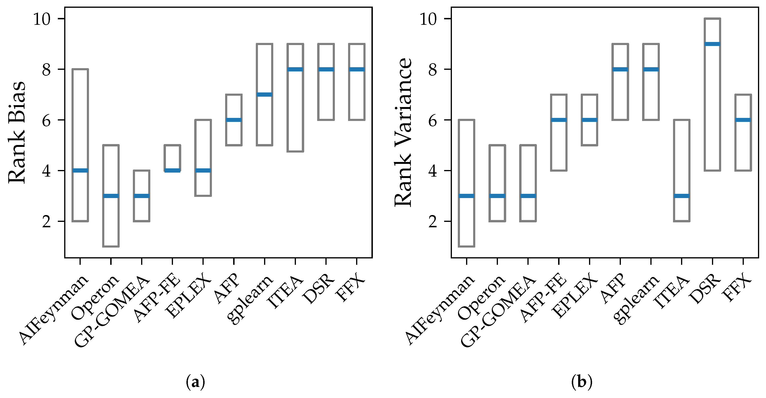
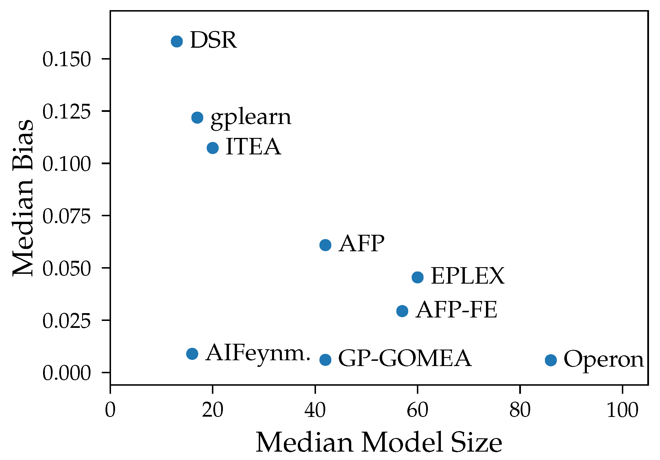
We show that both bias and variance increase with the test error of models over most algorithms. Exceptions are the algorithms AIFeynman, ITEA and FFX, whose error is primarily caused by bias. This is expected as stronger restrictions of the search space should lead to more similar outputs despite changes in training data but also to a consistent, systematic error in all models. Another assumption for the high bias for AIFeynman and FFX are their non-evolutionary heuristic search, which induces bias.

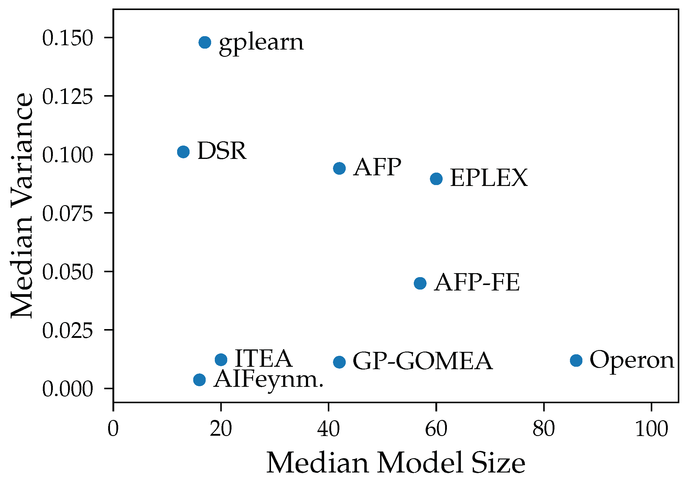
Our experiments prove our expectation that larger models tend to have smaller bias, except from FFX. However, despite the common assumption that larger models are susceptible to high variance, we could not observe a clear connection between those two properties in our analysis. The connection between variance and model size is distorted by the different median accuracy of the methods. Given that high accuracy is achieved both by algorithms with small and large models, also small variance occurs in algorithms with models of any size. E.g., Operon and GP-GOMEA provide the smallest error and variance across all noise levels, however, the size of their models differs clearly. While GP-GOMEA’s average model size ranks between the other algorithms, Operon found the largest models of all GP-based methods. However, this still implies, that even though Operon’s models are large and might look very different between multiple algorithm runs, their behavior on the Feynman datasets are very consistent.

This work is a first step towards the analysis of bias and variance in the symbolic regression domain. Although bias and variance belongs to the basic knowledge in machine learning, recent studies for other machine learning methods challenge the common understanding of this topic. Therefore, we also suggest further research in this direction for symbolic regression. The most obvious extension of our work would be an analysis on real world problems, as this work was restricted to generated benchmark data of problems with limited dimensionality. While the presence of actually unknown noise, an unknown ground truth and usually a too small number of observations in such scenarios make a fair comparison hard, it would give even further insight in the practicality of SR methods. Moreover, our analysis, especially regarding variance, was limited by the high accuracy of multiple algorithms on the given synthetic problems. Further research regarding the relationship between variance and model size would benefit from harder problems, where all algorithms yield a certain level of error. This would allow a more in-depth analysis of variance and highlight more differences between algorithms, especially between GP-GOMEA and Operon. Another SR-specific aspect for further research is the analysis of the symbolic structure of SR models. While this work only focuses on the behavior and output and therefore the semantic of models, another important aspect for practitioners is whether the formulas found in SR are similar from a syntactic perspective.