Article

Proactive Production Scheduling Approach for Off-Site Construction with Due Date Uncertainty

1
Architectural Engineering Program, School of Architecture, Seoul National University of Science and Technology, Seoul 01811, Republic of Korea
2
Department of Construction Management, College of Built Environments, University of Washington, Seattle, WA 98195, USA
*
Author to whom correspondence should be addressed.
Appl. Sci. 2024, 14(23), 11017; https://doi.org/10.3390/app142311017
Submission received: 18 October 2024 / Revised: 23 November 2024 / Accepted: 25 November 2024 / Published: 27 November 2024

Abstract

:
This study proposes a robust precast concrete (PC) production scheduling model for PC construction projects with schedule uncertainty by adopting a proactive scheduling approach. The proposed model consists of a PC production simulation module that simulates and evaluates the total tardiness of the schedule at a certain confidence level with contractor schedule uncertainty and a GA-based production schedule optimization module that finds an optimal schedule through iterative schedule generation and evaluation using a PC production simulation module. The experimental study shows that the proposed model can find the best schedule with 303.8 h of tardiness at a 100% confidence level, followed by NEHedd 324.7 h, basic GA 328.5 h, and EDD 335.8 h. The results of this study will help PC production schedulers to perform robustly despite contractors’ schedule changes and will thus contribute to the successful completion of PC construction projects.

1. Introduction

Off-site construction has increasingly gained attention as one of the solutions to address low productivity, high rates of accidents, and low quality in traditional on-site construction [1]. In precast concrete (PC) construction, which is a representative of the off-site construction methods, the PC components produced via an off-site manufacturer are delivered to an on-site one and then assembled. It can replace the traditional structural works consisting of formwork, rebar, and concrete pouring on-site by just the assembly of the PC components produced under the controlled off-site environment so that it can improve productivity and quality, with the possibility of accidents decreased [2].
PC production scheduling is vital for the successful completion of a project. It enables PC components produced by an off-site manufacturer to be delivered to each contractor’s site within their due date. Since PC component assembly is on the project’s critical path, any delay in delivering the PC components to the site will delay the subsequent work and extend the overall construction duration [3].
However, contractors’ schedule variability negatively influences the PC production schedule. A construction task can be delayed—or, in rare cases, completed ahead of schedule—due to various factors, such as unreliable planning, weather, equipment failures, labor shortages, or missing and incorrect data. These schedule changes related to on-site construction affect the due dates in off-site production and change the performance of the initial production schedule. The challenge of handling these inevitable disruptions is frequently viewed as a significant reason for the discrepancy between scheduling theory and its practical implementation in the industry [4].
The research in scheduling under uncertainty can be classified into the reactive scheduling approach and the proactive scheduling approach [5]. The reactive scheduling approach adjusts the schedule based on the actual conditions of the plant once uncertainties arise or unexpected events occur. However, implementing rescheduling strategies to address disruptions can be challenging and may result in ineffective or costly reconfigurations, as well as causing anxiety among the manufacturing staff [6]. In particular, PC suppliers might have to cancel a pre-scheduled job order or change the sequence of job orders due to a customer’s altered delivery schedule. Proactive scheduling generates schedules that are, in some sense, robust or insensitive to anticipated uncertainties, and it does not change schedules in the face of uncertainty. In many precast concrete (PC) suppliers, the production schedule is typically rigid, with monthly schedules fixed in advance, dictating resource planning. Despite occasional changes in delivery schedules requested by customers (construction contractors), most PC suppliers lack the flexibility to adjust their production schedules mid-cycle, highlighting the importance of developing proactive scheduling approaches. However, proactive scheduling approaches have not yet been sufficiently explored in PC production scheduling problems.
Therefore, this study aims to develop a robust PC production scheduling model for PC construction projects with schedule uncertainty by adopting a proactive scheduling approach. The proposed model consists of two modules: (1) a Monte Carlo (MC)-method-based PC production simulation module, which simulates and evaluates the total tardiness of the schedule with contractor schedule uncertainty; and (2) a genetic algorithm (GA)-based production schedule optimization module that finds a near-optimal schedule through iterative generation and evaluation using a PC production simulation module. It would help PC production schedulers to achieve robust schedule performance with contractors’ schedules changed, thereby leading to the PC components’ reliable and economical supply chain.
The rest of this study is organized as follows. Section 2 is a literature review of the relevant studies on PC production scheduling under uncertain environments. In Section 3, the proactive PC production scheduling model is proposed. In Section 4, through an experimental study, the proposed model is verified and discussed in a comparison study with two traditional dispatching rules, earliest due date (EDD) and NEHedd, as well as basic GA.

2. Relevant Studies on PC Production Scheduling Under Uncertain Environments

Production scheduling approaches under uncertain environments can be classified into two main categories: reactive and proactive approaches [6]. A reactive approach, such as rescheduling, plays a significant role in efficiently addressing unforeseen circumstances and reorganizing production resources and jobs promptly to minimize the losses resulting from changes [7]. On the other hand, the proactive approach considers stochastic and unforeseen events when creating the initial schedule. This approach aims to develop a robust and effective solution across nearly all scenarios involving uncertain parameters [8].
The existing studies on PC production scheduling under uncertain environments were systematically analyzed and categorized into reactive and proactive approaches as defined above.

2.1. Reactive Approach

The reactive approach has been extensively explored in the context of PC production scheduling. Chan and Wee [9] proposed a GA-based multi-heuristic schedule repair model for schedule disturbance resolution, such as completed element rejection and design change. Ko and Wang [10] proposed schedule adjustment principles to respond to demand variability, such as the magnitude and frequency of due date changes. Wang and Hu [11] developed a two-level rescheduling model for precast production with multiple production lines to minimize the rescheduling costs when due dates change. Ma et al. [12] proposed an approach for optimizing the shop floor rescheduling of multiple production lines for PC production in production emergencies such as machinery breakdown and rush orders. Kim et al. [2] proposed a dynamic PC scheduling model including a PC production simulation module and a new heuristic rule responding to due date changes. Du et al. [13] proposed the multi-objective genetic-algorithm-based dynamic flow shop scheduling model for prefabricated component production, which incorporates demand fluctuations such as the advancement of the due date, insertion of urgent components, and order cancellation. Wang et al. [14] proposed a hybrid rescheduling optimization model for precast production to minimize rescheduling costs and ensure on-time delivery under disruptions of machine breakdown. Kim et al. [3] proposed a PC production scheduling model that incorporates a deep reinforcement learning approach to minimize the total tardiness of PCPs by coping with dynamic store conditions in real time. Zhang et al. [15] proposed a three-layer scheduling disruption management model for scenarios in which order advancement and emergency order insertion occur concurrently in PC production workshops to minimize the maximum completion time, the earliness and tardiness penalties, and carbon emissions. Chen and Liu [16] proposed a Gene Expression Programming (GEP)-based optimized dynamic dispatching rule to respond to due date changes.
In summary, these studies highlight the diversity and adaptability of reactive approaches in addressing disruptions in PC production scheduling. They emphasize techniques such as genetic algorithms, simulation models, and heuristic methods to adjust schedules dynamically. Most of these approaches focus on minimizing tardiness or other performance penalties while responding to various disruptions like demand fluctuations, machine breakdowns, and urgent orders. However, while reactive strategies are effective in mitigating disruptions, their reliance on frequent schedule adjustments can lead to operational inefficiencies and increased complexity, posing challenges for practical implementation [6].

2.2. Proactive Approach

In contrast, the proactive approach has undergone comparatively limited exploration in PC production scheduling. Wang et al. [17] developed the simulation–GA hybrid model for PC production incorporating stochastic processing time, reflecting uncertain environments where the processing times follow a distribution. Their approach involved generating multiple near-optimal schedules to minimize delivery penalties through repeated GA runs in a deterministic environment. Subsequently, they conducted 100 simulations with stochastic processing times and selected the schedule that minimized the delivery penalties and production costs from the set of near-optimal schedules.
However, the approach of not considering uncertainty in the first stage when generating the schedule set can lead to several issues. Since the initial schedules are created in a deterministic environment, they may not accurately represent the impact of uncertainties. This results in schedules that are less resilient to fluctuations and unanticipated disruptions. While second-stage simulations aim to evaluate the performance of these schedules under uncertainty, post hoc corrections are often less effective because the initial schedules may deviate significantly from optimality when subjected to stochastic variations.
To address these limitations, this study introduces a proactive PC production scheduling model that explicitly incorporates due date uncertainty. By considering uncertainty at the initial scheduling stage, the proposed model could improve robustness and overall efficiency in handling dynamic and unpredictable environments.

3. Proactive PC Production Scheduling Model with Contractor Schedule Uncertainty

The proposed model aims to obtain a robust PC production schedule that is insensitive to anticipated contactor schedule uncertainties. The proposed model consists of two modules (Figure 1): (1) the MC-method-based PC production simulation module that simulates and evaluates the total tardiness of the schedule with contractor schedule uncertainty; (2) the GA-based PC production schedule optimization module that finds a near-optimal schedule through iterative schedule generation and evaluation using PC production simulation module.

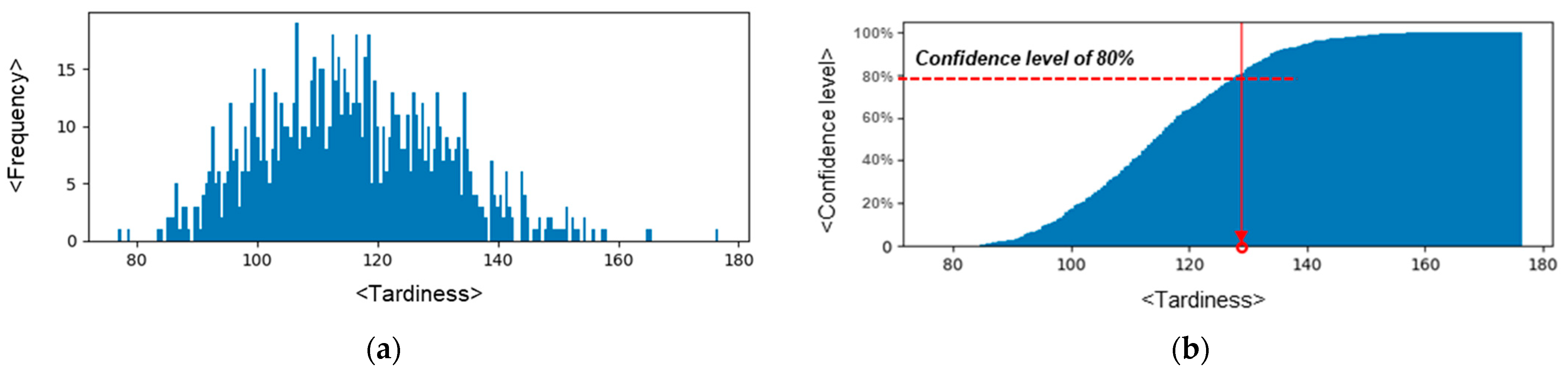
3.1. MC-Method-Based PC Production Simulation Module

PC production generally has six processes [2,18]: mold assembling (p1), placing of all embedded parts including rebars (p2), concrete casting (p3), concrete curing (p4), mold removal (p5), and product finishing (p6). All PC products follow the same production sequence regardless of their product types. Processing times are different depending on product types. The process can be classified in two ways. First, they can be categorized into uninterruptible and interruptible [11]. In the case of interruptible processes like p1, p2, p5, and p6, they must stop when the working hours end. Conversely, uninterruptible processes like p3 and p4 cannot be halted until they are completed. Second, the processes can be classified into parallel and non-parallel types [11]. A parallel process such as p4 immediately starts after p3 is completed without external resources, allowing multiple PC products to be concurrently processed. On the other hand, a non-parallel process cannot proceed with another product simultaneously; it must wait until the current PC product is fully completed.
Based on the PC production process, the MC-method-based PC production simulation module simulates and evaluates the total schedule tardiness at a specified confidence level considering the contractor’s schedule uncertainty (see Algorithm 1). This evaluation is conducted using the MC method, which is widely employed to numerically assess the expectations of functions of random variables [19].
Firstly, the simulation module accepts a job sequence (PC production schedule), the contractor’s due date reliability, the required confidence level (n), the number of simulations (S), and processing time ( p t t p ) as input variables. In each simulation, the dataset for the adjusted due date is generated based on the contractor’s due date uncertainty, modeled using a triangular distribution with three points (most pessimistic, most likely, and most optimistic values), which is particularly useful when a distribution is unknown due to data unavailability [20,21], in line 2. All processes except for concrete curing (p4) start the next job when the current job is finished. However, concrete curing (p4) will start immediately after the previous process (p3) has finished in lines 5–9. If the processing end time falls outside of working hours, the end time for each process is adjusted accordingly. For non-interruptible processes like concrete casting (p3), the end time is rescheduled to the start of the next working day, with the remaining processing time added in lines 10–12 since the process cannot be halted midway. The end time for concrete curing (p4), a non-interruptible process, is adjusted to the start time of the next day since curing can continue during non-working hours in lines 13–14. The end times for the other processes (p1, p2, p5, and p6) are extended to include non-working hours in line 16. Once the final process of the last job is completed in a simulation, tardiness is calculated using Equation (1) in line 19.
T a r d i n e s s = j = 1 J max ( f t 6 j c d j , 0 )
where J represents the total number of jobs; j denotes the index of jobs; f t 6 j refers to the finish time of job j in the 6th process; c d j denotes the changed due date of the jth job.
Algorithm 1: MC-method-based PC production simulation module
Input:job sequence, contractor’s due date reliability, confidence level ( n ) , # of simulations (S), processing time ( p t t p )
Output:tardiness at the confidence level ( n )
1:
2:
3:
4:
5:
6:
7:
8:
9:
10:
11:
12:
13:
14:
15:
16:
17:
18:
19:
20:
21:
22:
FOR simulation s in 1 to S DO
 Generate the changed due date dataset ( c d j 1 . . J ) based on the contractor’s due date reliability
 FOR process p in 1 to 6 DO
  FOR each j in job sequence DO
   IF  p = 4
    Set the start time of job j in process p ( s t p j ) as the finish time of job j in previous process p 1 ( f t p 1 j )
   ELSE
    Set the start time of job j in process p ( s t p j ) as the finish time of previous job j ( f t p j )
   Calculate the finish time ( f t p j ) by adding s t p j to the processing time of PC type t in process p ( p t t p )
   IF the finish time of the process ( f t p j ) is out of the working hour,
    IF  p = 3
     Skip the next day and add it to the processing time corresponding to the job j
    ELSE IF  p = 4 ,
     Set it to the next day
    ELSE
     Add non-working hours to it
  END FOR
END FOR
 Calculate tardiness
END FOR
Find tardiness at the confidence level ( n )  
RETURN tardiness at the confidence level ( n )
Then, the PC production process simulation is repeated for S simulations, and it returns the tardiness at the confidence level (n) in lines 21–22. Figure 2a shows an example of the distribution of tardiness after S (=1000) simulations under due date uncertainty; Figure 2b shows the corresponding cumulative distribution function (CDF) of tardiness, where the y-axis represents the confidence level (n). The figure highlights the position of tardiness at an 80% confidence level.

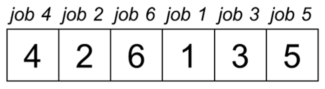
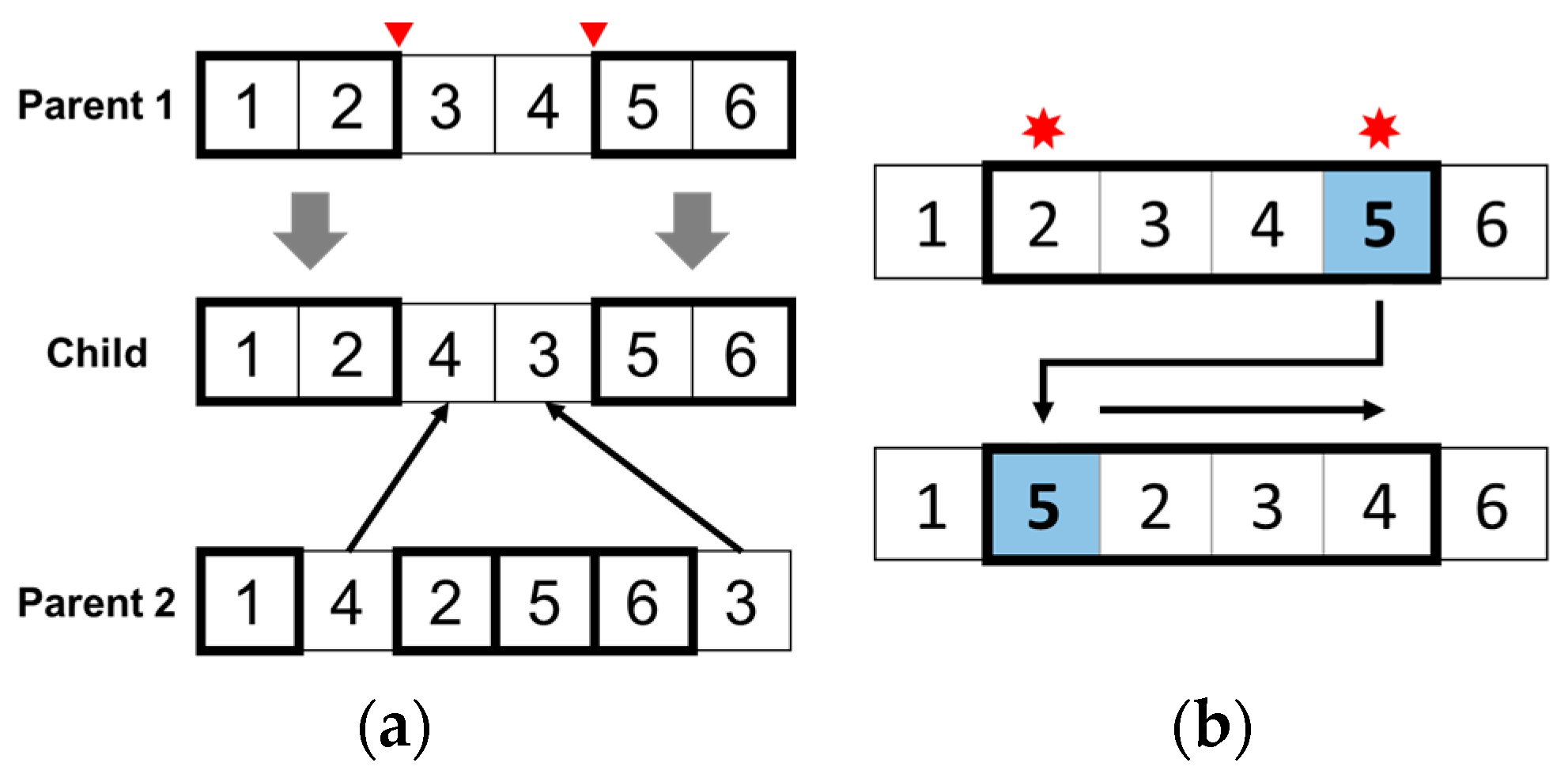
3.2. GA-Based PC Production Schedule Optimization Module

The GA-based PC production schedule optimization module identifies an optimal schedule through iterative generation, following the principles of natural evolution and evaluation using the PC production simulation module. Here, an optimal schedule is a schedule with the lowest tardiness value for a given confidence level (n) among many schedules.
This optimization module employs genetic algorithms (GAs), a search method inspired by Charles Darwin’s theory of natural evolution. This algorithm mimics the natural selection process, where the most suitable individuals are chosen to reproduce, thereby creating the next generation’s offspring. The main factor affecting PC production’s tardiness is the production sequence. For GA, production plans were encoded by job sequence, which is the permutation of given jobs, as shown in Figure 3. The string “426135” represents a job sequence where “job 4” is processed first, then “job 2” is processed, and so on.
The procedure of this module is shown in Algorithm 2.
Algorithm 2: GA-based PC production schedule optimization module
Input:population size, crossover rate, mutation rate, elite number, stopping criteria
Output:the best individual in a population
1:
2:
3:
4:
5:
6:
7:
8:
9:
Generate an initial population of candidate solutions to the problem
Evaluate the objective function of the individual in the population by Algorithm 1
WHILE NOT stopping criteria DO
 Perform selection of parents from the population
 Produce offspring by crossover between selected parents
 Perform mutation on offspring
Evaluate the objective function of offspring by Algorithm 1
 Make a new population by replacing the worst individual in offspring with the elite individual in the population
RETURN best individual in the population
Firstly, the optimization module takes population size, crossover rate, mutation rate, elite number, and stopping criteria. It randomly generates an initial population of candidate solutions to the problem based on the above encoding schema. The generated initial population is evaluated by its tardiness at confidence level (n), called fitness value, using the PC production simulation module.
Next, the module iterates the process until the stopping criteria are met. Initially, selection is performed by choosing parents from the population based on their fitness values using the roulette-wheel method [10,22,23]. Second, a crossover is applied to create a new candidate solution (i.e., offspring) from the two selected parent candidate solutions using the two-point crossover method, as illustrated in Figure 4a. Third, mutation is performed using shift mutation, which randomly selects two points and shifts them, as shown in Figure 4b [17,24]. Fourth, the PC production simulation module evaluates the offspring by their fitness value. Lastly, a new population is created by replacing the worst individual in offspring with an elite individual in the population.
Finally, when the stopping criteria are met, which in this study is determined by the number of iterations, the module returns the best individual in the population. Here, the best individual means the schedule with the lowest tardiness value at a given confidence level among all evaluated schedules.

4. Experimental Study

4.1. Overview

An experimental study was conducted to validate the proposed model by assessing tardiness values at a specified confidence level under due date uncertainty, comparing it against two traditional dispatching rules, such as EDD and NEHedd [25], and a basic GA. EDD is a scheduling rule that prioritizes tasks by selecting the next job in the queue based on the earliest due date. This approach ensures that tasks with the earliest deadlines are completed first, helping to minimize tardiness and meet due date requirements effectively. NEHedd arranges tasks in a non-decreasing order of due dates, adding each new task sequentially while inserting it in the optimal position to construct the final solution. The basic GA identifies a scheduling solution that minimizes tardiness, assuming no due date uncertainty. The experimental data in Table 1, showing the processing time for each process and PC product type, were obtained from Zhang et al. [15].
Contractors’ order information such as product type, due date, and quantity for contractors used in this experimental study are described in Table 2. The model assumes a total of 12 products, with 2 products assigned to each of the 6 contractors. Given the unique characteristics of construction sites, delays in due dates are more frequent than early completions [2]. Accordingly, the due date distribution was designed to reflect this tendency. The daily schedule assumes 10 h for work, 14 h for non-work activities, and 4 h for overtime. All experimental methods assume that, once the initial schedule is established, it cannot be adjusted, even if due dates change during production.
The parameters for the PC production simulation module were set to n of 100% and S of 1000. The GA parameters for the GA-based PC production schedule optimization module were set to a population size of 10, a crossover rate of 0.9, a mutation rate of 0.5, an elite number of 3, and stopping criteria of 1000 iterations based on references such as Murata et al. [24] and validated through testing to achieve both computational efficiency and solution quality. The proposed model and the other algorithms were written in Python 3.9, and the tests were conducted on a system with the following specifications: Windows 11, Intel i7-1260P CPU, and 16.0 GB RAM.

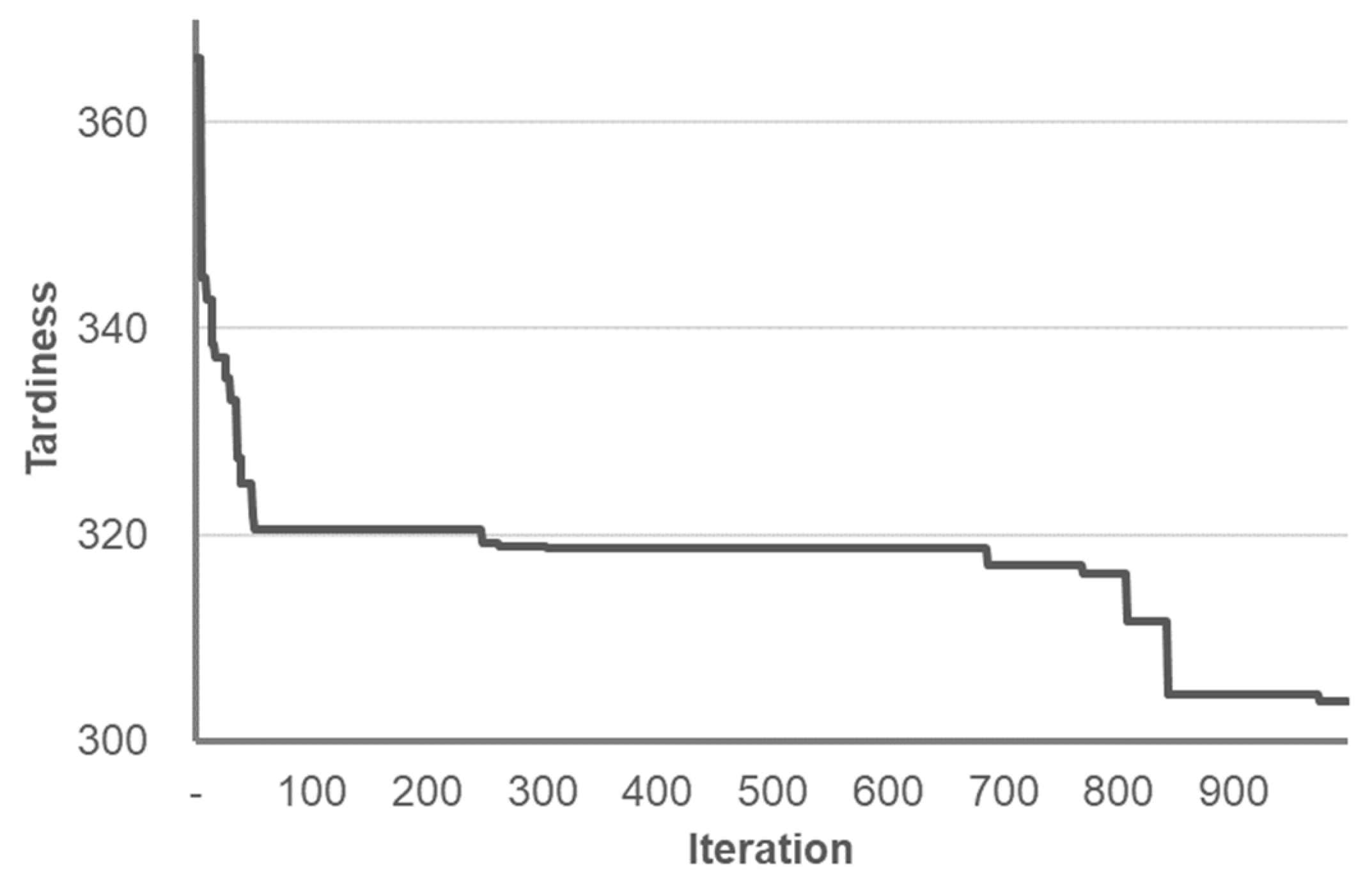
4.2. Results and Discussion

The fitness value of the GA converged over 1000 iterations, as shown in Figure 5. The fitness value of 303.8 represented the minimum tardiness at a 100% confidence level, achieved after 975 iterations.
Table 3 compares the performance of the proposed model against that of EDD, NEHedd, and basic GA, displaying the production sequences they generated and the corresponding tardiness results under two conditions: with and without due date uncertainty. When due date uncertainty was introduced, the proposed model achieved the lowest tardiness of 303.8 h at a 100% confidence level, followed by NEHedd with 324.7 h, basic GA with 328.5 h, and EDD with 335.8 h. Without due date uncertainty, the basic GA achieved the lowest tardiness of 114.5 h, followed by NEHedd with 115.5 h, the proposed model with 134.4 h, and EDD with 148.6 h. When comparing these results to the scenario where the due dates change, the corresponding tardiness values show confidence levels of 15%, 16%, 31%, and 39%. For example, the basic GA schedule demonstrated a tardiness of 114.5 h when there was no due date uncertainty (i.e., when the due date remained unchanged), which corresponds to a confidence level of 15% when the due date changes. In contrast, the proposed model exhibited a tardiness of 134.4 h without due date uncertainty, but this performance could be guaranteed at a higher confidence level of 31% when the due date changes. This result indicates that, without accounting for due date uncertainty, the reliability of the initially expected tardiness values is significantly lower.
Figure 6a shows that the distribution of tardiness in the proposed model is skewed towards smaller values compared to the other solvers. The cumulative distribution in Figure 6b further demonstrates that the proposed model identifies schedules with smaller tardiness values at the same confidence level compared to the other solvers.
Table 4 presents the optimal schedules obtained by varying the confidence level of the proposed model from 50% to 100%, alongside the schedules from the other three solvers for each confidence level. The proposed model shows that the tardiness value at the target confidence level is consistently lower than that of the other solvers.
The results suggest that the proposed model can effectively find a schedule that minimizes tardiness at the user’s desired confidence level under due date uncertainty. The proposed model presents a significant opportunity for enhancing production scheduling in the construction industry, particularly for small-sized prefabrication suppliers. One of the primary challenges faced by small-scale suppliers is the inability to quickly adjust production schedules in response to contractor-driven changes in due dates. The traditional scheduling methods lack the flexibility to respond to these fluctuations, which can lead to costly delays and inefficiencies. By integrating a robust, proactive scheduling approach, the proposed model addresses this issue, allowing suppliers to better manage their resource allocation and production timelines in a dynamic environment. It can be applied not only to PC production but also to other prefabricated products, such as MEP (mechanical, electrical, and plumbing) systems or façade elements. The flexibility and adaptability of this model make it a valuable tool in industries where the production schedules need to account for uncertainties in the delivery timelines.
However, the model operates under the assumption that suppliers have access to reliable data on the probabilistic distribution of due date changes for each order. This requirement poses a limitation as not all suppliers may have sufficient historical data to accurately predict how delivery dates may fluctuate. In cases where such data are unavailable, the suppliers will need to begin collecting and analyzing both the original and revised due dates for each project. These data are crucial for refining the model and accurately estimating the mean and variance of the due date uncertainty.
Despite this limitation, the proposed model offers considerable potential for improving supply chain reliability and reducing disruptions caused by unexpected schedule changes. By proactively managing uncertainties, suppliers can enhance their ability to meet delivery targets, minimize delays, and optimize resource utilization. Furthermore, as suppliers gather more data and improve their ability to estimate due date changes, the model will become even more effective at handling uncertainties, thereby offering long-term benefits in terms of cost efficiency and operational stability.
In conclusion, the proposed model contributes to the development of intelligent scheduling systems that can significantly improve the robustness and flexibility of production schedules in the prefabrication industry. It also highlights the importance of data collection and analysis in refining predictive models, thereby offering a practical solution to the challenges faced by suppliers in dynamic and uncertain production environments.

5. Conclusions

This study proposed a proactive scheduling model for PC production under due date uncertainty, which finds an optimal schedule insensitive to a priori anticipated contactor schedule uncertainties regarding tardiness. The proposed model comprises a PC production simulation module, which simulates and evaluates the total tardiness of the schedule under contractor schedule uncertainty, and a GA-based production schedule optimization module, which finds the optimal schedule through iterative generation and evaluation using the PC production simulation module. The proposed model was validated through the experimental study. As a result, the proposed model had the lowest tardiness of 303.8 h at the confidence level of 100%, followed by NEHedd 324.7 h, basic GA 328.5 h, and EDD 335.8 h. The results show that the proposed model can find a schedule with minimum tardiness given the uncertainty of the due date.
The proposed model can efficiently find an optimal schedule by simulating a vast number of scenarios under due date uncertainty, something that would be highly impractical to test in the real world without this approach. The optimal schedule created before production is robust to due-date changes without requiring production schedule changes that incur additional costs and time. Moreover, the proposed model can be used in other uncertain environments, such as equipment breakdown, failure of process operations, or processing time variation. Finally, the proposed model would contribute to the successful completion of the PC construction project by ensuring that the PC components are delivered to the contractor within their due date under due date uncertainty.
Even though we scientifically tested the promising potential of the proactive scheduling approach for PC production, there are some notable limitations. When simulating PC production considering the uncertain environment, we assumed the due date uncertainty distribution, which must be known in advance. Future research will examine the distribution of uncertain factors such as due dates, processing times, and equipment breakdowns. Additionally, the proactive scheduling cycle for PC production influences both overall performance and optimization runtime. In this study, 12 PC components were used for the experiments, and an optimal solution was achieved within 30 s through 1000 iterations of the GA. However, the longer the proactive scheduling cycle, the longer the optimization run time and the worse the performance of the established robust schedule can be. Of course, the optimization runtime or the performance of the robust schedule will not entirely dominate the scheduling cycle. In practice, the optimal scheduling cycle should consider various conditions in the production environment, such as resource planning cycles and lead times. Therefore, we recommend that future studies analyze the proactive and reactive scheduling cycles to optimize schedule performance and runtime.
Finally, while this study focused on due date uncertainty and tardiness to develop a robust schedule, PC construction projects may encounter various other uncertainties, as well as objectives such as makespan or earliness. The future research will explore scheduling models that optimize multiple objectives within multi-uncertainty environments.

Author Contributions

Conceptualization, T.K. and Y.-W.K.; methodology, Y.-W.K.; validation, T.K.; formal analysis, T.K. and Y.-W.K.; investigation, T.K.; resources, T.K.; data curation, T.K.; writing—original draft preparation, T.K. and Y.-W.K.; writing—review and editing, T.K. and Y.-W.K.; visualization, T.K.; supervision, Y.-W.K.; project administration, Y.-W.K.; funding acquisition, T.K. and Y.-W.K. All authors have read and agreed to the published version of the manuscript.

Funding

This study was financially supported by Seoul National University of Science and Technology.

Institutional Review Board Statement

Not applicable.

Informed Consent Statement

Not applicable.

Data Availability Statement

The data present in this study are available on request from the corresponding author.

Conflicts of Interest

The authors declare no conflicts of interest.

References

  1. Jang, J.; Ahn, S.; Cha, S.H.; Cho, K.; Koo, C.; Kim, T.W. Toward productivity in future construction: Mapping knowledge and finding insights for achieving successful off-site construction projects. J. Comput. Des. Eng. 2021, 8, 1–14. [Google Scholar] [CrossRef]
  2. Kim, T.; Kim, Y.W.; Cho, H. Dynamic production scheduling model under due date uncertainty in precast concrete construction. J. Clean. Prod. 2020, 257, 120527. [Google Scholar] [CrossRef]
  3. Kim, T.; Kim, Y.W.; Lee, D.; Kim, M. Reinforcement learning approach to scheduling of precast concrete production. J. Clean. Prod. 2022, 336, 130419. [Google Scholar] [CrossRef]
  4. Goren, S.; Sabuncuoglu, I. Robustness and stability measures for scheduling: Single-machine environment. Iie Trans. 2008, 40, 66–83. [Google Scholar] [CrossRef]
  5. Herroelen, W.; Leus, R. Robust and reactive project scheduling: A review and classification of procedures. Int. J. Prod. Res. 2004, 42, 1599–1620. [Google Scholar] [CrossRef]
  6. Bonfill, A.; Espuna, A.; Puigjaner, L. Proactive approach to address the uncertainty in short-term scheduling. Comput. Chem. Eng. 2008, 32, 1689–1706. [Google Scholar] [CrossRef]
  7. Novas, J.M.; Henning, G.P. A reactive scheduling approach based on domain-knowledge. Comput. Aided Chem. Eng. 2009, 27, 765–770. [Google Scholar]
  8. Baohua, W.; Shiwei, H.E. Robust optimization model and algorithm for logistics center location and allocation under uncertain environment. J. Transp. Syst. Eng. Inf. Technol. 2009, 9, 69–74. [Google Scholar]
  9. Chan, W.T.; Wee, T.H. A multi-heuristic GA for schedule repair in precast plant production. In Proceedings of the 13th International Conference on Automated Planning and Scheduling (ICAPS), Trento, Italy, 9–13 June 2003; pp. 236–245. [Google Scholar]
  10. Ko, C.H.; Wang, S.F. GA-based decision support systems for precast production planning. Autom. Constr. 2010, 19, 907–916. [Google Scholar] [CrossRef]
  11. Wang, Z.; Hu, H. Dynamic response to demand variability for precast production rescheduling with multiple lines. Int. J. Prod. Res. 2018, 56, 5386–5401. [Google Scholar] [CrossRef]
  12. Ma, Z.; Yang, Z.; Liu, S.; Wu, S. Optimized rescheduling of multiple production lines for flowshop production of reinforced precast concrete components. Autom. Const. 2018, 95, 86–97. [Google Scholar] [CrossRef]
  13. Du, J.; Dong, P.; Sugumaran, V. Dynamic production scheduling for prefabricated components considering the demand fluctuation. Intell. Autom. Soft Comput. 2020, 26, 715–723. [Google Scholar] [CrossRef]
  14. Wang, Z.; Liu, Y.; Hu, H.; Dai, L. Hybrid rescheduling optimization model under disruptions in precast production considering real-world environment. J. Constr. Eng. Manag. 2021, 147, 04021012. [Google Scholar] [CrossRef]
  15. Zhang, R.; Feng, X.; Mou, Z.; Zhang, Y. Green optimization for precast production rescheduling based on disruption management. J. Clean. Prod. 2023, 420, 138406. [Google Scholar] [CrossRef]
  16. Chen, J.; Liu, X. GEP algorithm-based optimization method for PCs production scheduling under due date variation. In Proceedings of the 2023 4th International Conference on Computer Engineering and Application (ICCEA), Hangzhou, China, 7–9 April 2023; pp. 347–352. [Google Scholar]
  17. Wang, Z.; Hu, H.; Gong, J. Framework for modeling operational uncertainty to optimize off-site production scheduling of precast components. Autom. Constr. 2018, 86, 69–80. [Google Scholar] [CrossRef]
  18. Benjaoran, V.; Dawood, N.; Hobbs, B. Flowshop scheduling model for bespoke precast concrete production planning. Constr. Manag. Econ. 2005, 23, 93–105. [Google Scholar] [CrossRef]
  19. Ghasemi, A.; Farajzadeh, F.; Heavey, C.; Fowler, J.; Papadopoulos, C.T. Simulation optimization applied to production scheduling in the era of industry 4.0: A review and future roadmap. J. Ind. Inf. Integr. 2024, 39, 100599. [Google Scholar] [CrossRef]
  20. Wanke, P.; Ewbank, H.; Leiva, V.; Rojas, F. Inventory management for new products with triangularly distributed demand and lead-time. Comput. Oper. Res. 2016, 69, 97–108. [Google Scholar] [CrossRef]
  21. Liang, T.F. Application of interactive possibilistic linear programming to aggregate production planning with multiple imprecise objectives. Prod. Plan. Contr. 2007, 18, 548–560. [Google Scholar] [CrossRef]
  22. Goldberg, D.E. Genetic Algorithms in Search, Optimization and Machine Learning; Addison-Wesley: Boston, MA, USA, 1989. [Google Scholar]
  23. Reeves, C.R. A genetic algorithm for flowshop sequencing. Comput. Oper. Res. 1995, 22, 5–13. [Google Scholar] [CrossRef]
  24. Murata, T.; Ishibuchi, H.; Tanaka, H. Genetic algorithms for flowshop scheduling problems. Comput. Ind. Eng. 1996, 30, 1061–1071. [Google Scholar] [CrossRef]
  25. Kim, Y.D. Heuristics for flowshop scheduling problems minimizing mean tardiness. J. Oper. Res. Soc. 1993, 44, 19–28. [Google Scholar] [CrossRef]
Figure 1. Framework of the proposed model.
Applsci 14 11017 g001
Figure 2. Example of a robust schedule solution at the confidence level ( n ): (a) histogram of tardiness after 1000 simulations; (b) cumulative frequency of tardiness after 1000 simulations. The red dotted line and red arrow indicate the 80% confidence level and the corresponding tardiness, respectively.
Applsci 14 11017 g002
Figure 3. Encoding schema.
Applsci 14 11017 g003
Figure 4. Operators for GA: (a) two-point crossover; (b) shift mutation. The red symbols indicate two selected points.
Applsci 14 11017 g004
Figure 5. Evolutionary curve of GA.
Applsci 14 11017 g005
Figure 6. Test results on different solvers: (a) distribution of tardiness; (b) cumulative distribution of tardiness.
Applsci 14 11017 g006
Table 1. Processing time for each PC product type.
Product TypeProcessing Time (h)
p1p2p3p4p5p6
P12.03.62.5101.01.1
P23.13.21.0101.52.1
P32.22.81.7101.00.8
P40.81.91.2101.01.2
P51.22.02.6100.80.9
P63.04.01.1101.62.5
P71.12.21.6101.02.1
Table 2. Order information.
ContractorProduct TypeDue Date
(Most Pessimistic, Most Likely, Most Optimistic Value)
C1P1(24, 24, 24)
P2(24, 24, 24)
C2P2(0, 24, 72)
P3(0, 24, 72)
C3P3(0, 48, 120)
P4(0, 48, 120)
C4P4(0, 48, 132)
P5(0, 48, 132)
C5P5(0, 72, 168)
P6(0, 72, 168)
C6P6(12, 96, 204)
P7(12, 96, 204)
Table 3. Experimental results based on different solvers.
SolverProduction Sequencew/Due Date Uncertaintyw/o Due Date Uncertainty
Tardiness (h)Confidence
Level (%)
Tardiness (h)Confidence Level (%)
EDD[1, 2, 3, 4, 5, 6, 7, 8, 9, 10, 11, 12]335.8100148.639
NEHedd[6, 1, 3, 8, 5, 4, 7, 9, 2, 10, 12, 11]324.7100115.516
basic GA[6, 4, 2, 8, 5, 7, 3, 9, 1, 10, 12, 11]328.5100114.515
Proposed model[6, 1, 2, 4, 7, 3, 9, 8, 5, 10, 12, 11]303.8100134.431
Table 4. Experimental results based on a confidence level.
SolverProduction
Sequence
Tardiness Based on a Confidence Level (h)
50%60%70%80%90%100%
EDD[1, 2, 3, 4, 5, 6, 7, 8, 9, 10, 11, 12]155.6169.4183.9202.1228.7324.7
NEHedd[6, 1, 3, 8, 5, 4, 7, 9, 2, 10, 12, 11]165.4179.6195.8216.0249.0335.8
basic GA[6, 4, 2, 8, 5, 7, 3, 9, 1, 10, 12, 11]159.0170.5184.1204.9227.9328.5
Proposed model with 50%[7, 1, 2, 4, 8, 6, 3, 9, 5, 10, 12, 11]138.8155.2171.8185.9213.5343.1
    ‘’   with 60%[7, 1, 2, 4, 8, 6, 3, 5, 9, 10, 12, 11]139.2155.0171.6185.8213.0343.3
    ‘’   with 70%[6, 1, 2, 4, 8, 3, 7, 5, 9, 10, 12, 11]142.0156.1169.8190.4216.4316.5
    ‘’   with 80%[7, 1, 2, 4, 6, 8, 3, 5, 9, 10, 12, 11]139.6155.3171.3185.4213.5342.5
    ‘’   with 90%[7, 1, 2, 4, 8, 6, 3, 5, 9, 10, 12, 11]139.2155.0171.6185.8213.0343.3
    ‘’   with 100%[6, 1, 2, 4, 7, 3, 9, 8, 5, 10, 12, 11]149.3161.5177.9194.5224.7303.8
Bold and italics indicate the lowest tardiness value within the same confidence level.
Disclaimer/Publisher’s Note: The statements, opinions and data contained in all publications are solely those of the individual author(s) and contributor(s) and not of MDPI and/or the editor(s). MDPI and/or the editor(s) disclaim responsibility for any injury to people or property resulting from any ideas, methods, instructions or products referred to in the content.

