Dynamic Prediction of Shale Gas Drilling Costs Based on Machine Learning

Abstract

Shale gas, a significant recoverable natural gas resource trapped in shale formations, represents a significant energy reservoir. Although China has significant recoverable shale gas reserves, the challenge of controlling drilling costs remains a critical barrier to efficient development. This study presents a novel stacked ensemble learning model that integrates support vector machine (SVM) and long short-term memory (LSTM) networks to improve the accuracy of shale gas drilling cost prediction. The methodology consists of three main phases. First, we constructed a comprehensive, multidimensional spatiotemporal dataset of shale gas drilling costs. Second, we used Gradient Boosting Decision Tree (GBDT) modelling to rank the importance of various factors influencing drilling costs. Finally, we developed a stacked ensemble learning model combining SVM and LSTM architectures to achieve superior cost prediction accuracy. Experimental results demonstrate the effectiveness of the model, with the coefficient of determination (R²) improving from 0.25189/0.33834 (traditional SVM/LSTM models) to 0.55934. Model validation using selected well investment data from the Changning Block shows promising performance, achieving a Mean Absolute Percentage Error (MAPE) of 6.41%, with optimal prediction accuracy in the medium investment range (60–70 million yuan). This innovative approach provides a reliable tool for predicting shale gas drilling costs and offers new methodological perspectives for cost reduction strategies. The results contribute significantly to the sustainable development of shale gas resources and provide valuable insights for industry practitioners and researchers in the fields of energy economics and resource management.

1. Introduction

As a cornerstone of global energy production, the oil and gas industry has historically faced challenges in accurately predicting and optimising drilling costs [1]. As exploration and production activities expand into more complex geological formations and extreme environments, the need for sophisticated cost prediction and optimisation techniques becomes increasingly important [2].

Drilling operations represent a significant proportion of the total expenditure incurred in oil and gas exploration and production. Industry reports indicate that drilling costs can account for up to 50% of the total cost of well development, with this percentage often increasing in challenging environments, such as ultra-deepwater or unconventional reservoirs [3]. The ability to accurately predict and optimise these costs is not only a matter of financial prudence, but also a critical factor in project feasibility, risk management and strategic decision making [4]. With volatile oil prices and increased environmental scrutiny, the need for cost-effective and efficient drilling operations has never been more pressing.

Traditionally, the estimation of drilling costs has relied on empirical models and expert judgement [5]. While these methods have proven valuable, they often fail to capture the full complexity of drilling operations, particularly in new or challenging environments. The inherent uncertainty of subsurface conditions, coupled with the dynamic nature of the drilling process, often results in significant discrepancies between estimated and actual costs [6]. Such inaccuracies can lead to project overruns, sub-optimal resource allocation and, in some cases, the abandonment of otherwise viable prospects.

The advent of big data analytics, machine learning and artificial intelligence has ushered in a transformative era in drilling cost forecasting and optimisation [7]. These technologies can process vast amounts of historical and real-time data, identify complex patterns, and generate insights that were previously unattainable [8]. In the context of shale gas development and exploitation, understanding the cost structure and making dynamic predictions about cost changes is critical [9]. This enables the formulation of effective development strategies and informed decision making.

The rest of the paper is organised as follows: Section 2 presents the related work on machine learning, respectively; Section 3 analyses the data characteristics of shale gas drilling costs and the existing related machine learning models and proposes a stacked integrated learning scheme based on SVM + LSTM; Section 4 shows the experimental results and analyses them, and finally summarises the work and proposes a further optimisation scheme.

2. Related Work

2.1. Feature Engineering and Selection for Drilling Costs

Feature engineering and selection play a critical role in improving the accuracy and effectiveness of drilling cost prediction models. Numerous studies have focused on developing novel methods in this area.

Sajadfar and Ma [10] introduced a hybrid cost estimation algorithm that uses a feature-oriented data mining approach to improve the accuracy of cost estimation for engineering projects, particularly in drilling operations. This innovative method integrates domain expertise with data-driven analysis to effectively extract and select features relevant to cost estimation. By combining feature-driven conceptual cost estimation with advanced data mining techniques, the framework demonstrates improved performance and reliability compared to traditional cost estimation methods.

Barbosa et al. [11] reviewed various machine learning methods applied to the prediction and optimisation of drilling penetration rates (ROP). They found that methods such as artificial neural networks, support vector machines and random forests were successful in modelling complex ROP relationships with drilling parameters and formation properties. Key advantages of these approaches include improved prediction accuracy, the ability to handle non-linear effects, and the potential for real-time optimisation. This analysis provides a data-driven approach to decision making for drilling operation costing. In a separate study, Ren et al. [12] focused on optimising features for predicting drilling rates based on real-time data. Their approach allows for dynamic selection and optimisation of features in response to new data arrivals, improving the adaptability of the model to changing drilling conditions. This adaptive capability leads to more accurate predictions in the context of geological uncertainties.

Eskandarian et al. [13] used a comprehensive data mining approach to estimate the rate of penetration and emphasised the importance of feature ranking. Their research highlighted the need to identify and prioritise the most influential features for accurate ROP prediction, using neural networks, rule-based models and feature ranking techniques to improve prediction accuracy. In addition, Pan et al. [14] proposed a methodology for predicting drilling costs based on self-adaptive differential evolution and support vector regression. This approach automatically selects optimal features and parameters, thereby improving prediction accuracy and generalisation ability. Taken together, these studies highlight the importance of advanced feature engineering and selection methods in improving the accuracy and reliability of drilling cost predictions [15].

2.2. Machine Learning and Ensemble Learning for Drilling Cost Prediction

The application of machine learning and ensemble learning techniques has significantly transformed drilling cost forecasting, providing improved accuracy and robustness compared to traditional methods. Robi Polikar [16] proposed the use of machine learning methods for cost forecasting in the energy sector and subsequently introduced an ensemble approach to validate its effectiveness in improving prediction accuracy. Xu et al. [17] developed a Genetic Algorithm–Back Propagation (GA–BP) neural network-based model specifically for ultra-deep well drilling cost prediction. This model exploits the global optimisation capabilities of genetic algorithms in conjunction with the learning capabilities of back-propagation neural networks and demonstrates particular effectiveness in dealing with the inherent complexities of ultra-deep well drilling. Liu et al. [18] introduced a stacked generalisation ensemble model to optimise and predict the rate of penetration (ROP) in gas wells. A case study conducted in Xinjiang showed that ensemble methods significantly improved prediction accuracy compared to individual models. The stacked model outperformed single models such as random forest and gradient boosting, demonstrating its superior predictive capability.

Hegde and Gray [9] investigated the potential of machine learning and data analytics to improve drilling efficiency in the vicinity of neighbouring wells. Their methodology uses historical data from neighbouring wells to optimise drilling parameters and reduce costs. It was shown that transfer learning techniques can be effectively used to apply knowledge from one well to improve predictions for nearby wells. Yehia et al. [19] conducted a comparative analysis of machine learning techniques for predicting ROP in geothermal wells, using a case study from the FORGE research site. They evaluated the performance of algorithms, such as random forests, gradient boosting and neural networks, and found that random forests achieved the highest accuracy in their case study. The authors highlight the importance of representative training data and feature engineering for effective ROP modelling.

Nautiyal and Mishra [20] explored the potential of machine learning to improve drilling efficiency in the oil and gas industry. The study demonstrated the potential of AI-driven approaches to optimise drilling operations and reduce associated costs. The researchers investigated the applicability of a number of machine learning algorithms to different aspects of drilling optimisation. Matinkia et al. [21] developed a novel model for predicting the rate of penetration in drilling operations using convolutional neural networks (CNN). The approach demonstrated the potential of deep learning techniques to capture complex patterns in drilling data, thereby enabling more accurate ROP predictions. Tewari et al. [22] proposed an intelligent drilling methodology for oil and gas wells using response surface methodology and artificial bee colony optimisation. Their hybrid approach showed promise in optimising drilling parameters and reducing costs. These studies illustrate the growing prevalence of advanced machine learning and ensemble techniques in addressing the complexities of drilling cost prediction and optimisation and represent a significant advance in the field.

2.3. Dynamic Cost Prediction for Shale Gas Drilling and Development

The dynamic nature of shale gas drilling and development requires the use of advanced predictive models that can adapt to changing conditions and incorporate a range of factors that influence costs over time.

Eltrissi et al. [23] proposed a machine learning framework for optimising drilling operations. Their approach integrates real-time sensor data, geological information, and machine learning models to provide decision support for adjusting drilling parameters such as weight on bit and speed. The authors demonstrate the framework’s ability to improve ROP and reduce drilling time and costs compared to conventional optimisation methods. Similarly, Yang et al. [24] focused on optimising drilling parameters for target wells using machine learning and data analytics. Their research highlights the importance of adaptive models that can account for the unique characteristics of each well within shale gas fields. By integrating data pre-processing, feature selection and various machine learning algorithms, they effectively optimised drilling parameters in a dynamic context.

Elahifar and Hosseini [25] developed an automated real-time prediction system for geological formation tops during drilling operations. Although their study did not directly address cost prediction, their machine learning solution applied to the Norwegian Continental Shelf illustrates the potential of real-time data integration within dynamic drilling models that can significantly influence cost estimates. Their system achieved high accuracy in predicting formation tops, potentially leading to reduced drilling times and associated costs. In addition, Sabah et al. [26] introduced a machine learning approach for predicting the rate of penetration (ROP) based on petrophysical and mud logging data. This method, which is adaptable for real-time predictions, has significant implications for dynamic cost estimation in shale gas drilling. The researchers compared different machine learning algorithms and found that ensemble methods were most effective in addressing the complexities associated with ROP prediction. Together, these studies underscore the growing importance of dynamic, adaptive models capable of real-time cost prediction and optimisation in the rapidly evolving landscape of shale gas drilling and development.

2.4. Intelligent Drilling Systems and Automation

Recent advances in intelligent drilling systems and automation technologies represent a significant trend in improving drilling efficiency and cost effectiveness. Li et al. [27] provide an invaluable contribution to the field of intelligent drilling and completion technologies. They cover a wide range of topics, including real-time data acquisition, the development of automated decision-making frameworks, and the formulation of sophisticated control algorithms. Their findings illustrate how these innovations facilitate cost reduction and improve the efficiency of drilling operations. Yang et al. [28] explore the application of artificial intelligence (AI) to improve drilling status detection in the oil drilling sector. Their empirical research demonstrates the ability of AI techniques to automatically detect and respond to varying drilling conditions, thereby minimising human error and increasing operational efficiency.

Bello et al. [29] provide a thorough review of AI methods applied to the design and operation of drilling systems. They examine various AI techniques and their potential applications in various aspects of drilling, including well planning and real-time optimisation. Their analysis highlights the ability of AI to optimise decision-making processes, ultimately leading to reduced drilling costs. Gan et al. [30] propose a multi-objective optimisation approach for operational drilling parameters in complex geological contexts. Their method aims to improve drilling efficiency by simultaneously optimising multiple parameters, thus demonstrating the effectiveness of advanced optimization techniques in reducing both drilling costs and duration.

Taken together, these studies highlight the transformative potential of intelligent systems and automation technologies in drilling operations. By harnessing these advances, the industry can achieve substantial cost savings and significant improvements in operational efficiency.

2.5. Economic Analysis and Cost Optimization in Drilling Operations

Several studies have focused on the economic aspects of drilling operations and methods for optimising costs through various techniques. Ozdemir et al. [31] conducted a comprehensive drilling evaluation and cost analysis of oil and gas wells drilled onshore in Turkey. Their study provided valuable insights into the factors influencing drilling costs in specific geological and economic contexts, emphasising the importance of region-specific cost models. Nwanwe and Teodoriu [32] introduced a matrix for selecting and comparing drilling methods and technologies for a wide range of applications. Their approach facilitates decision making by evaluating different drilling technologies based on both technical and economic criteria, potentially leading to more cost-effective choices in drilling operations.

Purba et al. [33] investigated the optimisation of geothermal drilling costs in Indonesia, taking into account various influencing factors. Their research highlighted the unique challenges and opportunities associated with geothermal drilling and showed that cost optimisation strategies can vary significantly depending on the type of drilling operation. Bani Mustafa et al. [34] focused on improving drilling performance by optimising controllable drilling parameters. Their results indicated that careful parameter optimisation could result in significant cost savings and efficiency improvements in drilling operations. Taken together, these studies highlight the importance of comprehensive economic analysis and strategic optimisation in effectively managing drilling costs.

3. Materials and Methods

3.1. Shale Gas Cost Structure Explained

As an unconventional natural gas resource, the development and production of shale gas is not only of great importance to the energy industry, but also has a significant impact on economic, environmental and social development. To fully understand the cost structure of shale gas, several factors need to be carefully considered, including exploration and development, production and transportation costs.

First, exploration and development costs are the primary expenditure in shale gas projects. These costs include geological exploration, drilling, reservoir evaluation, engineering design and equipment procurement. Shale gas resources are typically located in deep formations, and the exploration and development process requires significant capital and human resources to determine the presence of natural gas and estimate recoverable reserves [35]. In addition, the complexity of shale gas reservoirs requires the use of advanced technology and equipment for development, which further increases exploration and development costs.

Second, production costs are a critical factor affecting the economic viability of shale gas development. In the shale gas development process, production costs mainly include well operating costs, hydraulic fracturing operations and capacity maintenance [36]. Compared to conventional natural gas production, shale gas production requires extensive hydraulic fracturing to release the natural gas, which significantly increases production costs. In addition, the extended production cycle of shale gas requires continuous investment in maintaining production capacity and implementing post-production management, further increasing production costs.

In addition, transportation costs are a significant component of the shale gas cost structure. Shale gas development often takes place in remote areas or regions with complex geological conditions, and the transportation, processing and storage of natural gas requires significant resources and capital investment. In particular, the construction, operation and maintenance costs of transport pipelines have a direct impact on the overall economics of shale gas development [37].

Beyond the primary factors mentioned above, the cost structure of shale gas is influenced by several additional elements, including technological progress and innovation, regulatory policy, capital market conditions and geological characteristics. Technological progress and innovation can reduce exploration and development costs while improving production efficiency, thereby reducing overall costs. Changes in policy and regulation have a direct impact on the cost of shale gas projects through fiscal policy, environmental standards and exploration and production licences. Capital market conditions and the investment environment affect the cost of financing and investment decisions for shale gas projects. In addition, regional geological conditions influence the complexity of shale gas exploration and development, which in turn affects the cost structure [38].

Therefore, elucidating the cost structure of shale gas requires consideration of multiple aspects, including exploration and development, production and transportation costs, as well as the influence of technological, political, capital and geological factors. Understanding these elements is crucial for formulating appropriate development strategies, optimising production costs and enhancing competitiveness [39].

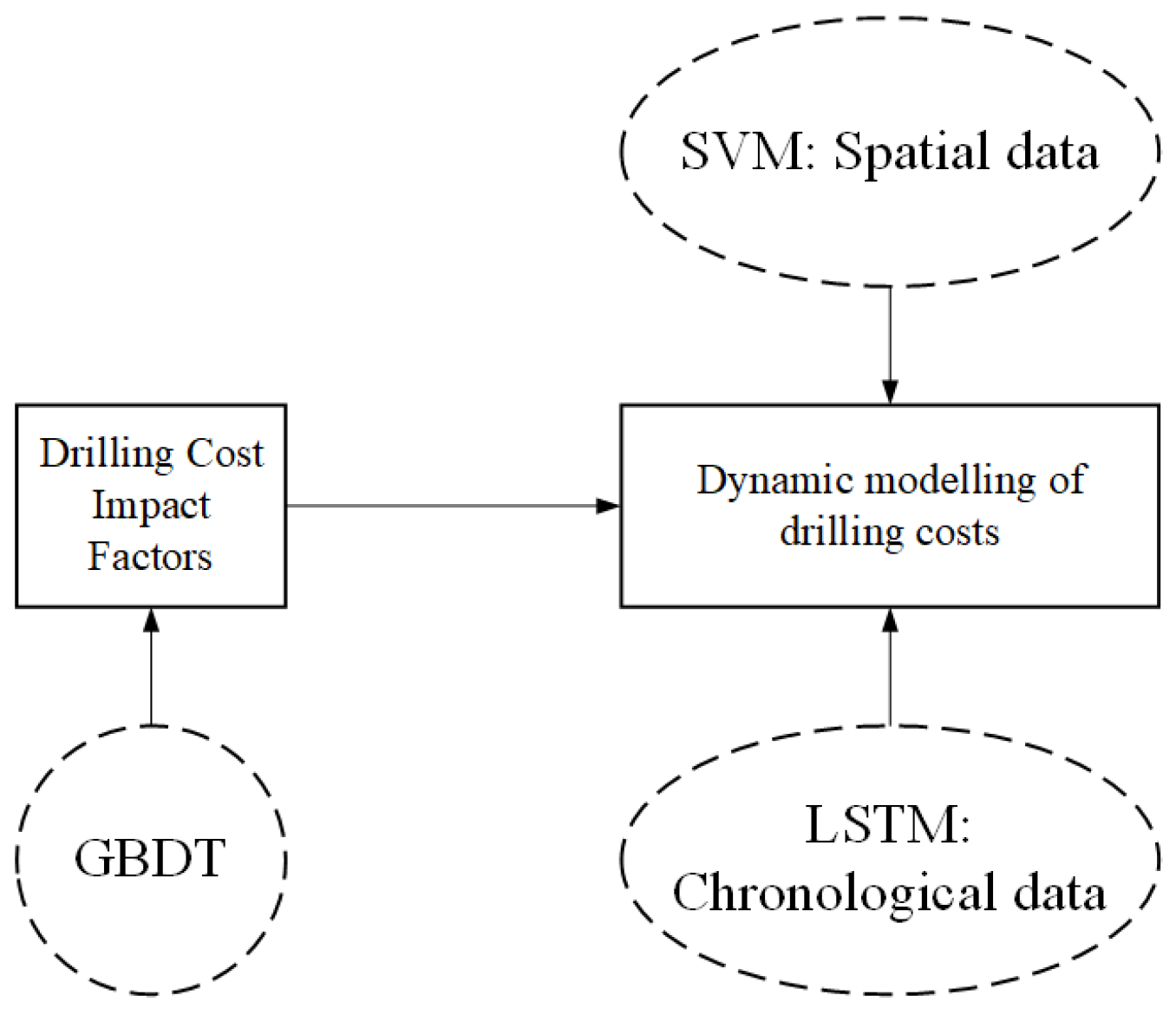
3.2. Model and Proposed Method

1. 

GBDT

Gradient Boosting Decision Trees (GBDT) is a machine learning algorithm that performs prediction and regression analysis by integrating multiple decision trees. GBDT employs an iterative training process whereby multiple weak classifiers (decision trees) are progressively enhanced, thus improving the overall predictive performance of the model [40]. This method enables the calculation of the importance indices for each feature, thus facilitating the identification of the factors that exert the greatest influence on the target variable. To gain a comprehensive understanding of the fundamentals and implementation of the GBDT algorithm, it is recommended to consult the paper by Chen and Guestrin [41] and the study by Alonso-Español et al. [42].

2. 

SVM

Support Vector Machine (SVM) is a versatile machine learning algorithm used for both classification and regression tasks. It aims to find the optimal hyperplane that maximizes the margin between classes in the feature space [43]. In this study, the SVM model is employed for regression analysis of the factors influencing shale gas drilling costs, with the objective of obtaining accurate and reliable predictions. For a comprehensive understanding of the principles and applications of SVMs, it is recommended to consult the seminal work by Vapnik [44] and the review by Smola and Schölkopf [45].

3. 

LSTM

Long Short-Term Memory (LSTM) is a specialised type of Recurrent Neural Network (RNN) designed to efficiently process sequence data [46]. In the context of time series analysis, LSTM is capable of learning patterns and trends, as well as capturing the dynamic effects of different features on costs, thereby facilitating more accurate forecasting. To gain a comprehensive understanding of the LSTM structure and its application in sequence modelling, it is recommended to consult the original paper by Gers et al. [47] and the review by Greff et al. [48].

4. 

Stacking Integrated Learning Models

Stacking is an advanced integrated learning technique that improves prediction performance by systematically combining SVM and LSTM models [49]. This methodology involves several sequential steps: first, the dataset is partitioned into training and test sets; then, the SVM and LSTM base models are trained independently; these base models then generate predictions for the test set; these predictions then serve as novel features for the metamodel input construction; the metamodel is trained; and finally, the trained stacking model processes new data for prediction. This integrated approach effectively synthesises the complementary strengths of different models, thereby improving overall prediction accuracy.

The research framework uses GBDT, SVM and LSTM models in a collaborative manner to optimise the cost of drilling individual wells in shale gas operations. As shown in Figure 1, the methodology demonstrates the integration of learning through the GBDT model for a comprehensive analysis of cost influencing factors. The selected features initially serve as inputs to the GBDT model, which is trained to elucidate and quantify their respective influences on shale gas drilling costs. The model autonomously learns feature relationships and corresponding weights, generating an interpretable framework for both cost prediction and factor analysis. The output of the GBDT model provides a hierarchical ranking of the factors influencing drilling costs, along with precise quantification of each feature’s contribution. This analytical framework enables researchers and decision makers to understand the differential impact of different factors on costs, providing a scientific basis for drilling process optimisation and cost control.

Figure 1. Multi-model collaborative application construction idea diagram.

In addition, a two-dimensional integrated learning model is implemented to improve the accuracy and reliability of dynamic cost prediction in shale gas drilling. The stacking methodology synthesises the predictive outputs of the LSTM and SVM models, effectively exploiting their complementary advantages. The LSTM model is particularly adept at time series analysis, performing sophisticated feature extraction to capture temporal dynamics and cyclical patterns. Conversely, SVM models, on the other hand, are good at spatial data analysis and can effectively establish decision boundaries for classification or regression of multivariate data sets, especially when the sample size is limited. The choice of SVR as a metamodel in the SVM model not only inherits the principle of structural risk minimisation of the SVM, but also constructs a robust nonlinear regression estimator through the ε-insensitive loss function in a small sample learning scenario.

The results of both cost prediction models are comprehensively evaluated to assess predicted costs from multiple analytical perspectives. This evaluation facilitates the selection of optimal algorithms and parameter configurations, ultimately improving prediction accuracy and providing robust decision support.

3.3. Optimisation Programme and Valuation Indicators

• Grid search represents a systematic approach to hyperparameter optimisation in machine learning models. The method functions by exhaustively testing predefined combinations of hyperparameters, including those related to learning rate, regularisation strength, and tree depth, through the utilisation of cross-validation for the assessment of model performance. Although grid search is an effective method for identifying optimal hyperparameter combinations and improving model performance through parallel computing, its efficiency is significantly reduced when dealing with large search spaces [50].
• K-fold cross-validation represents a robust methodology for the assessment of machine learning models, whereby the dataset is partitioned into K equal subsets (commonly 5 or 10), with one subset designated as the validation set and the remaining K-1 subsets serving as the training set. This process is repeated K times, with each part serving as the validation set in turn, and the results are averaged to obtain the final performance evaluation. This approach effectively utilises all available data and helps to optimise model hyperparameters while avoiding the limitations of single train-test splits [51].
• Mean Absolute Error (MAE) and Root Mean Square Error (RMSE) are two commonly used error assessment metrics to quantify the deviation between the predicted and actual values of a model [52]. MAE is the average of the sum of the absolute values of the differences between all predicted values and the true values, which measures the average deviation of the predicted values from the true values. The smaller the value of MAE, the smaller the deviation of the model’s predicted results from the true values, indicating better prediction performance. RMSE is the square root of the average of the squares of the prediction errors. It not only focuses on the deviation between the predicted value and the true value, but also amplifies the effect of larger deviations, so RMSE is more sensitive to larger errors.

  $$MAE={\displaystyle \frac{1}{\mathrm{n}}}{\displaystyle {\sum }_{i=1}^n\left|y^{(i)}-{\widehat{y}}^{(i)}\right|}$$

  (1)

  $$RMSE=\sqrt{{\displaystyle \frac{1}{\mathrm{n}}}{\displaystyle {\sum }_{i=1}^n{(y^{(i)}-{\widehat{y}}^{(i)})}^2}}$$

  (2)

  where ${\mathrm{y}}^{(i)}$ and ${\widehat{\mathrm{y}}}^{\left(\mathrm{i}\right)}$ are the true and predicted values of the sample, respectively, and n is the total number of samples.
• Decision coefficient. The evaluation measures the strength of the model by calculating the coefficient of determination, where the value is in the range of (0, 1) and, the closer its value is to 1, the better the model is fitted [52].

  $$R^2={\displaystyle \frac{\sum _{i=1}^n{({\widehat{\mathrm{y}}}^{\left(\mathrm{i}\right)}-\overline{{\widehat{\mathrm{y}}}^{\left(\mathrm{i}\right)}})}^2}{\sum _{i=1}^n{({\mathrm{y}}^{\left(\mathrm{i}\right)}-\overline{{\mathrm{y}}^{\left(\mathrm{i}\right)}})}^2}}$$

  (3)

  where ${\mathrm{y}}^{\left(\mathrm{i}\right)}$ is the true value, $\overline{{\mathrm{y}}^{\left(\mathrm{i}\right)}}$ is the average value of the true value, ${\widehat{\mathrm{y}}}^{\left(\mathrm{i}\right)}$ is the predicted value, and $\overline{{\widehat{\mathrm{y}}}^{\left(\mathrm{i}\right)}}$ is the average value of the predicted value.

4. Experiments and Results

4.1. Data Sources

This study analyses data from 564 shale gas development wells and 31 shale gas appraisal wells in the Sichuan Basin during the period 2015–2022. The data sources of the study mainly include two dimensions: first, production and operation data such as engineering data, construction parameters and cost data within the southwest oil and gas field enterprises; and second, time series data, such as macroeconomic indicators and other time series data from research institutions, government statistical offices and industry consulting firms, as well as spatial dimensions, such as geological conditions, covering more than 36 indicator items in total.

In the process of data preparation, it is very important to select appropriate eigenvalues because the choice of eigenvalues directly affects the subsequent analysis and modelling results. According to the research content of this project, we selected 36 variables for the study, as shown in Table 1.

Table 1. Variable for shale gas drilling costs.

Index	Variable Name	Index	Variable Name	Index	Variable Name	Index	Variable Name
1	Well number	10	Fracturing pump pressure	19	Annual GDP	28	Per capita consumption expenditure of urban residents
2	Well type	11	Fluid intensity	20	Consumer Price Index (CPI)	29	Per capita consumption expenditure of rural residents
3	Commissioning time	12	Total sand addition	21	Total imports and exports	30	Total retail sales of consumer goods
4	Well depth	13	Number of platform wells	22	Average daily temperature	31	Number of public buses and trolley buses in the municipal area
5	Horizontal section length	14	Shale yards verified single well EUR	23	Number of bridges	32	Number of taxis in the municipal area
6	Actual fracturing length	15	Degree of policy support	24	Area of real roads in cities	33	Number of people employed in the transport storage and postal sector
7	Number of fracturing sections	16	Geological conditions	25	Total wages of on-the-job workers in the municipal area	34	Number of post offices
8	Sand addition intensity	17	Degree of scientific and technological expenditures	26	Number of employed persons	35	Cargo turnover
9	Fracturing displacement	18	Corporate Commodity Price Index (CGPI)	27	Average number of employed workers	36	Investment in drilling and completion of wells

4.2. Data Processing

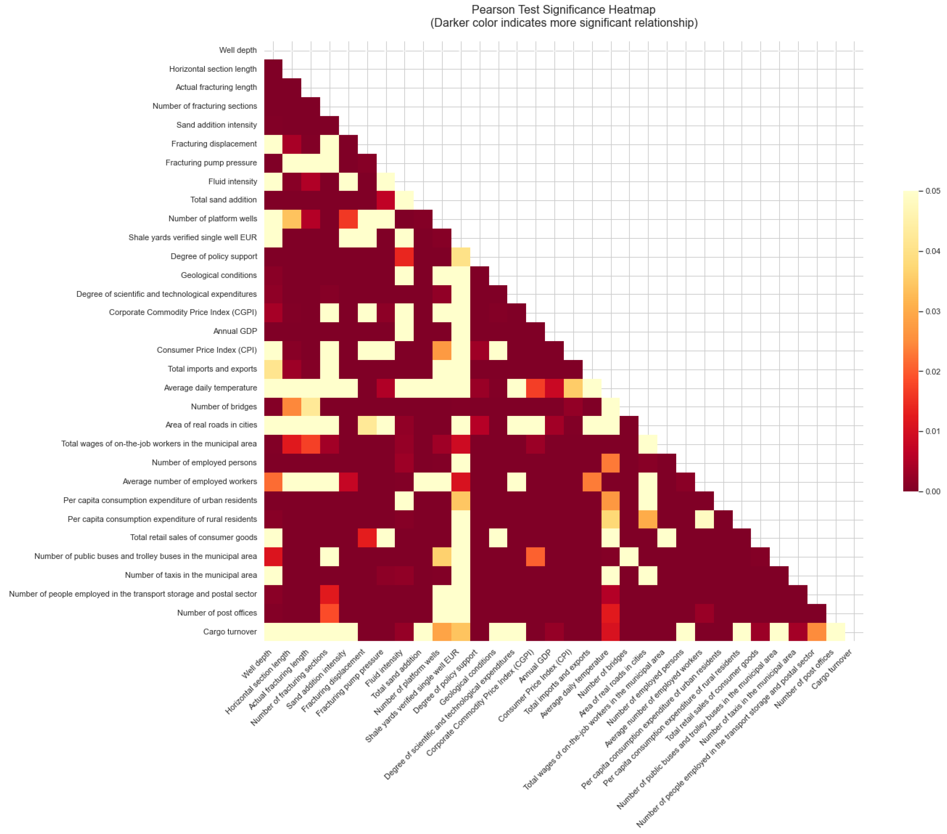
After the construction of the spatio-temporal big data set was completed, the data integrity was first systematically tested. The test results showed that part of the dataset was missing in 2021–2022, for which a data processing scheme was developed. The complete analytical dataset was then constructed through a series of data pre-processing steps, including data de-weighting, missing value filling, outlier identification and processing, data structure optimisation, interpolation calculation and standardisation processing.

4.3. Pearson Test

In this study, a multidimensional correlation analysis of drilling engineering parameters and their influencing factors was carried out using Pearson correlation analysis statistics, a number of correlations with different levels of significance were found, reflecting the existence of a significant correlation between the factors, and the results are shown in Table 2.

Table 2. Pearson test results for different shale gas drilling costs features.

Index	Variable Name	Pearson Correlation	p-Value (Max)
1	Actual fracturing length	0.091781	0.042279
2	Annual GDP	0.119031	0.008352
3	Area of real roads in cities	−0.097925	0.030209
4	Average daily temperature	0.094083	0.037349
5	Average number of employed workers	0.102400	0.023397
6	Cargo turnover	0.095721	0.034148
7	Consumer Price Index (CPI)	0.095045	0.035440
8	Corporate Commodity Price Index (CGPI)	−0.104520	0.020664
9	Degree of policy support	−0.125078	0.005562
10	Degree of scientific and technological expenditures	0.418286	0.000001
11	Fluid intensity	−0.110961	0.013989
12	Fracturing displacement	−0.091786	0.042268
13	Fracturing pump pressure	0.122340	0.006700
14	Geological conditions	0.159277	0.000401
15	Horizontal section length	−0.095850	0.033905
16	Number of bridges	0.238878	0.000001
17	Number of employed persons	−0.146708	0.001126
18	Number of fracturing sections	0.106456	0.018414
19	Number of fracturing sections	0.106456	0.018414
20	Number of people employed in the transport storage and postal sector	−0.101383	0.024816
21	Number of platform wells	−0.094622	0.036268
22	Number of public buses and trolley buses in the municipal area	−0.551319	0.000000
23	Number of taxis in the municipal area	0.130173	0.003896
24	Per capita consumption expenditure of rural residents	0.605843	0.000001
25	Per capita consumption expenditure of urban residents	−0.169663	0.000161
26	Sand addition intensity	−0.108594	0.016181
27	Shale yards verified single well EUR	−0.092772	0.040095
28	Total imports and exports	0.102400	0.023397
29	Total retail sales of consumer goods	0.134243	0.002906
30	Total sand addition	−0.159130	0.000406
31	Total wages of on-the-job workers in the municipal area	0.278988	0.000001
32	Well depth	0.092305	0.041111

Through a detailed analysis of the p-values, these variables were classified into three levels according to their level of significance:

• Analysis of factors with very high significance

The study showed that there was a significant correlation between technical engineering parameters and economic indicators. The level of technological expenditure showed a significant positive correlation (r = 0.418, p ≈ 0.000001) with the total wages of workers, indicating a significant link between drilling technology inputs and labour costs. The level of infrastructure support also showed synergistic effects, with the positive correlation between the number of bridges and the actual road area (r = 0.239, p ≈ 0.000001) reflecting the systematic nature of drilling project support facilities. These associations reveal the complexity of the cost components of drilling projects.

2.

Analysis of highly significant factors

Fracturing technical parameters show significant technical correlations. Fracturing pump pressure and total sand addition show a positive correlation (r = 0.122, p = 0.007), reflecting the intrinsic link between fracturing process parameters, while the negative correlation between total sand addition and platform wells (r = −0.159, p = 0.0004) reveals the influence of scale effect on material utilisation efficiency. Meanwhile, the correlation (r = 0.159, p = 0.0004) between geological conditions and the company’s commodity price index suggests that geological factors have a significant impact on drilling costs.

3.

Analysis of factors influencing moderate significance

A weak but significant correlation was found between drilling parameters and external factors. The positive correlation between the actual fracturing length and the number of bridges (r = 0.092, p = 0.042) and the negative correlation between the horizontal section length and the number of platform wells (r = −0.096, p = 0.034) reflect the need for comprehensive consideration of external conditions in engineering design. Particularly noteworthy is the correlation between the degree of political support and fluid intensity (r = −0.111, p = 0.014) and shale gas single well EUR (r = −0.093, p = 0.040), suggesting that the political environment has a moderating effect on the selection of technical drilling parameters and final production capacity.

As shown in Figure 2, the results of the statistical analysis based on Pearson correlation analysis allow us to scientifically verify the rationality of the selected indicators. The analysis shows that multi-level correlation analysis reveals the complex interactions between technical parameters, economic indicators, geological conditions and political environment in drilling technology. There is an obvious correlation between the technical parameters of the drilling project, geological conditions and the level of infrastructure support, and these have an important impact on the implementation of the drilling project, which should be taken into account in the cost forecast, and the policy environment plays an important role in regulating the choice of drilling project technology and improving economic efficiency.

Figure 2. Pearson Test Significance Heatmap.

4.4. Descriptive Analysis of Data

In this study, descriptive statistical analysis of shale gas related data is shown in Table 3, which is the frequency distribution table of the time of production, from which it is known that the valid number of samples for the data is 490.

Table 3. Frequency distribution of commissioning times.

	Frequency	Percentage	Effective Percentage	Cumulative Percentage
2015	20	4.1	4.1	4.1
2016	24	4.9	4.9	9.0
2017	16	3.3	3.3	12.2
2018	38	7.8	7.8	20.0
2019	100	20.4	20.4	40.4
2020	157	32.0	32.0	72.4
2021	74	15.1	15.1	87.6
2022	61	12.4	12.4	100.0
Total	490	100.0	100.0

Figure 3 show that the shale gas drilling activity shows significant uneven distribution characteristics between the different years. Among them, the drilling activity in 2020 is the most active, accounting for 32.0% of the total, closely followed by 2019 and 2021, accounting for 20.4% and 15.1%, respectively. In stark contrast, drilling activity was relatively subdued between 2015 and 2017, creating a distinctly concave area on the radar chart, with 2017 being particularly inactive, accounting for just 3.3% of the total.

Figure 3. Frequency and percentage analysis of shale gas drilling.

Comparing the two key metrics of drilling frequency (blue curve) and percentage distribution (green curve), it can be seen that both show very similar distribution patterns. The cumulative percentage shows a gradual upward trend over time, a feature that strongly confirms the apparent cyclical nature of shale gas production activities.

Table 4 shows the results of descriptive statistical analysis of macroeconomic indicators: CGPI enterprise commodity price index, annual GDP (billion yuan), consumer price index CPI, total imports and exports (billion yuan) and average daily temperature (°C).

Table 4. Descriptive statistics of macroeconomic indicators.

	CGPI Corporate Goods Price Index	Annual GDP (Billion Yuan)	Consumer Price Index CPI	Total Import and Export (Billion Yuan)	Average Daily Temperature (°C)
Effective number of cases	490	490	490	490	490
Minimum value	92.7	871.36	100.1	24.88	0.5
Maximum value	110.1	1614.47	102.6	49.38	31
Mean value	101.13	1364.12	101.82	37.69	18.48
Standard Deviation	4.00	190.01	0.88	6.89	8.18

Table 5 shows the mean, median, variance, minimum and maximum values of each drilling parameter and drilling and completion investment obtained through descriptive statistical analysis.

Table 5. Descriptive statistics of drilling engineering parameters.

Variant	Mean	Median	Variance	Minimum Value	Maximum Value
Well depth (metres)	4875.57	4900	222,555.88	3330	6325
Horizontal section length (metres)	1662.14	1500	127,824.33	850	3100
Actual fracturing length (metres)	1579.62	1470	147,103.84	236	3166
Number of fracturing sections (sections)	25.00	24	37.73	4	51
Strength of sand addition (Mg/m)	2.30	2.32	0.36	0.81	4.70
Fracturing displacement (m3/min)	0.427	0.447	0.005	0.241	1.618
Fracturing pump pressure (MPa)	75.81	75.72	73.53	50.5	96.68
Intensity of fluid used (m2/m)	29.16	28.77	14.37	16.09	44.58
Total sand addition (Mg)	3688.65	3369.04	2,431,753.95	319.48	11,813.79
Number of platform wells (ports)	4.82	5	2.12	1	8
Verification of single well EUR by shale yard (109 m3)	1.14	1.12	0.15	0.19	2.42
Investment in drilling and completing wells (106 yuan)	64.3429	62.9134	10,597.0741	37.4399	120.3020

Before implementing machine learning algorithms, data partitioning for model training and testing is essential. The data set is systematically divided into two distinct components: the training set and the test set. The training set is used to calibrate the model by adjusting its parameters according to the specified machine learning algorithm, with the goal of optimising the fit between model predictions and actual outcomes within the training data [53].

The test set remains completely independent of the training process and is used solely to evaluate the final performance of the model at the end of training. This approach provides robust insights into the model’s ability to generalise when applied to previously unseen, independent data. In this research, a 70:30 ratio was used to partition the data into training and test sets. This partitioning method proves particularly effective for model training and validation when applied to large datasets characterised by relatively uniform distributions.

4.5. Drilling Cost Indicator Construction

With today’s rapid advances in big data and artificial intelligence technologies, large-scale data processing and mining is playing an increasingly important role in the analysis of drilling cost drivers and the development of optimisation strategies. Traditional cost analysis methods often show limitations in considering indirect factors and fail to fully exploit the potential of big data analysis, thereby limiting the effectiveness of cost optimization initiatives. As a result, this research is based on a comprehensive big data analytics framework that examines multiple factors that influence shale gas drilling costs. The primary objective is to develop a holistic cost analysis methodology that is capable of thoroughly incorporating various influencing factors, which is of significant value in optimising shale gas drilling costs.

As shown in Table 6, this study incorporates indicators across 13 different dimensions to provide a comprehensive analysis of the factors influencing shale gas drilling costs. In addition, through an extensive literature review and consideration of data accessibility, 36 specific variables were systematically selected for investigation during the data preparation phase.

Table 6. Drilling cost indicator construction system.

Classification	Variant	Classification	Variant
Basic information	Well number, type of well and time of commissioning	Road conditions	Number of bridges, real urban road area
Engineering parameters	Well depth, horizontal section length, actual fracturing length, number of fracturing sections, sand addition intensity, fracturing displacement, fracturing pump pressure, fluid intensity used, total sand addition, number of platform wells, shale yard verification of individual wells EUR	Macroeconomic	Corporate Goods Price Index (CGPI), annual GDP, Consumer Price Index (CPI), total imports and exports
Policies	Level of policy support	Labour Force	Total wage bill of workers in employment in the municipal area, number of employed persons
Geological conditions	Per capita water resources	Consumption Level	Per capita consumption expenditure of urban residents, per capita consumption expenditure of rural residents and total retail sales of consumer goods
Science and Technology Innovation	Degree of expenditure on science and technology	Accessibility	Public Tram Passenger Volume in Municipal Districts and Number of Taxis in Municipal Districts
Investment costs	Investment in drilling and completion of wells	Logistics	Transport, storage and postal employment, number of post offices and cargo turnover
Temperature	Daily average temperature values	Weather conditions	Daily average temperature value

4.6. Feature Importance Calculation Based on GBDT Algorithm

This study aims to use the GBDT model to quantify and elucidate the factors influencing shale gas drilling costs and their respective degrees of influence through the analysis of pre-processed data. The model inputs consist of pre-processed data covering a wide range of variables affecting shale gas drilling costs, including engineering parameters, construction processes, settlement data, macroeconomic indicators, meteorological and natural disaster information, geological conditions, transport logistics, living conditions and regulatory policies. The integration of these comprehensive features into the GBDT model facilitates the training process in order to explain and quantify their respective impacts on shale gas drilling costs. The model autonomously identifies the intricate relationships and weights between the features, generating an interpretable framework for both drilling cost prediction and factor analysis [51]. The output of the GBDT model provides a hierarchical ranking of the factors influencing drilling costs, accompanied by a precise quantification of the specific contribution of each feature. The GBDT model training process generated importance indices for the features included in each shale gas cost prediction model. The six most important influencing factors identified through this analysis are presented in Table 7.

Table 7. Analysis of Factors Affecting Shale Gas Costs.

Rank	Factor	Importance Index	Impact Level	Detailed Description
1	Number of Fracturing Sections	0.3462	High Impact	Increasing the number of fracturing sections can enhance shale gas production but leads to higher costs in drilling, fracturing, and equipment.
2	Well Depth	0.1806	High Impact	Greater well depth results in higher exploration and development costs, requiring longer drilling time, larger drilling equipment, and more investment.
3	Number of Platform Wells	0.1281	High Impact	Increasing platform wells improves extraction efficiency and reduces production costs by centralizing multiple wells in one location, saving on drilling and production equipment.
4	Actual Fracturing Length	0.0644	Medium Impact	Longer fracturing lengths can increase shale gas production but require more fracturing materials and fluids, resulting in higher construction costs.
5	Fracturing Pump Pressure	0.0589	Medium Impact	Higher pump pressure can increase well production but results in increased energy consumption and equipment costs.
6	Sand Intensity	0.0402	Medium Impact	Higher sand intensity can improve fracturing results and increase production but increases the amount and cost of sand and fracturing fluid used.
7+	Other Factors	<0.0400	Low Impact	Other listed factors have relatively low impact on shale gas costs. While they may have some influence in specific situations, their impact needs to be considered from a comprehensive perspective.

Notes: Impact Level Classification: High Impact: Importance Index > 0.1000; Medium Impact: Importance Index 0.0400–0.1000; Low Impact: Importance Index < 0.0400.

4.7. Results

Stacking model parameter optimisation aims to determine the optimal configuration of base models (SVM and LSTM), the appropriate number of base models and the most effective combination method. Several combinations and ratios are systematically tested and evaluated using the validation set. Subsequently, the most appropriate meta-model is selected for the final prediction based on the outputs of the base models. The grid search methodology is used to evaluate different parameter combinations, with selection based on quantitative performance metrics. To ensure model efficiency and parameter optimisation, the data is systematically partitioned into training, validation and test sets, followed by evaluation of the model’s predictive ability on the test set. This methodological approach effectively addresses potential overfitting issues and provides a more robust assessment of the model’s ability to generalise.

To evaluate the effectiveness of the SVM_LSTM stacked model, a comparative analysis is performed against the individual SVM and LSTM models. To visually demonstrate the advantages of the SVM_LSTM methodology, the predicted values from the test data are compared across all three methods, as shown in Figure 4. The analysis shows that, while both the traditional SVM and LSTM models demonstrate satisfactory drilling cost prediction capabilities after training and generally meet the required prediction requirements, the SVM_LSTM stacked model exhibits improved prediction accuracy.

Figure 4. Comparison of predicted values of models test data.

4.8. Analysis of Results

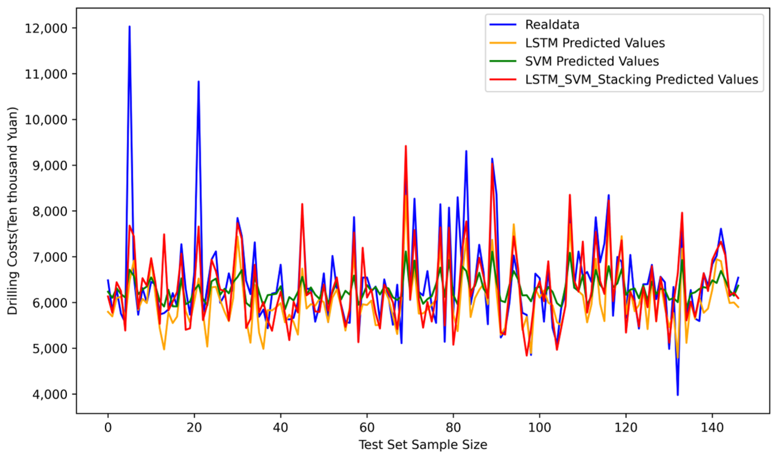
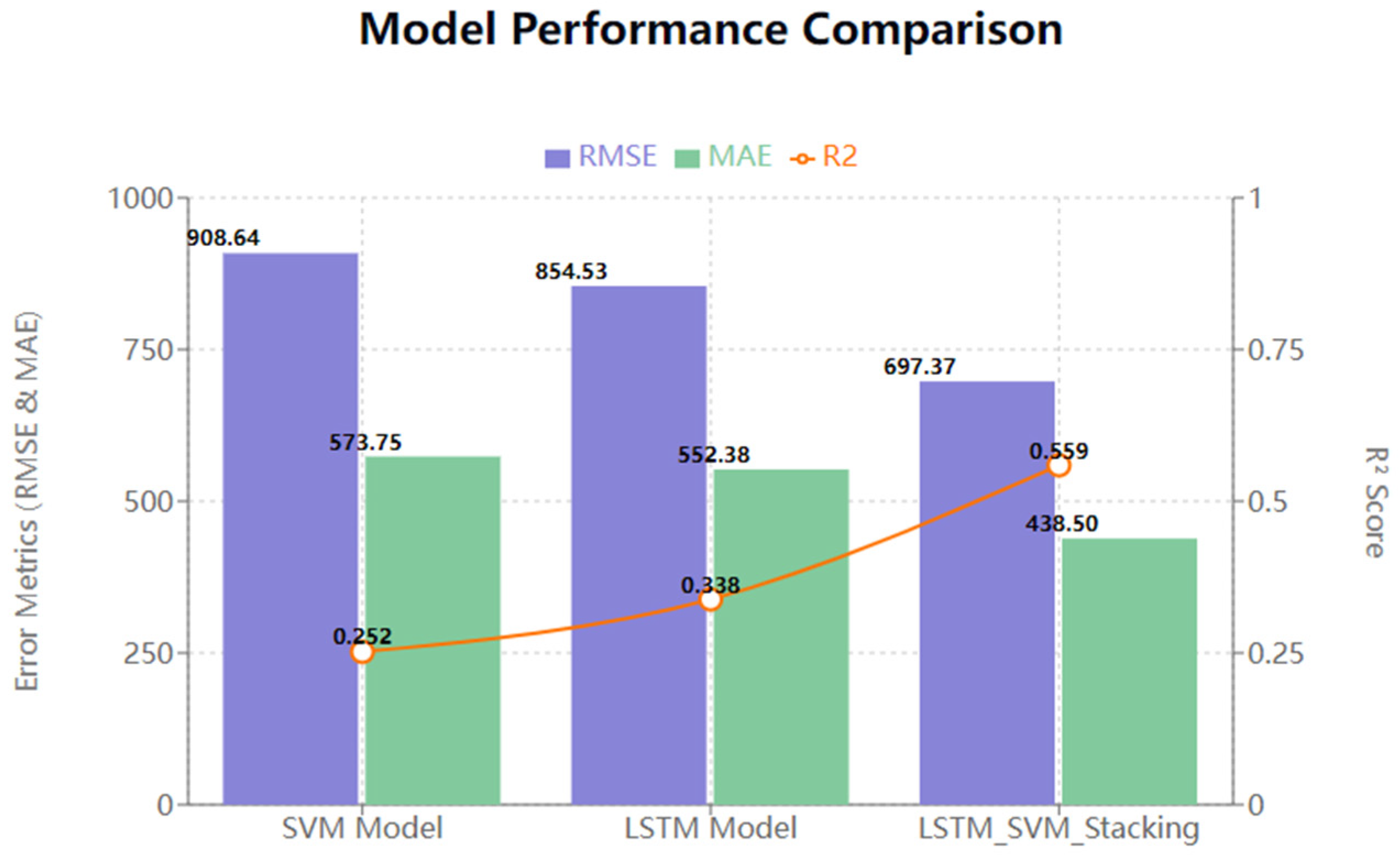
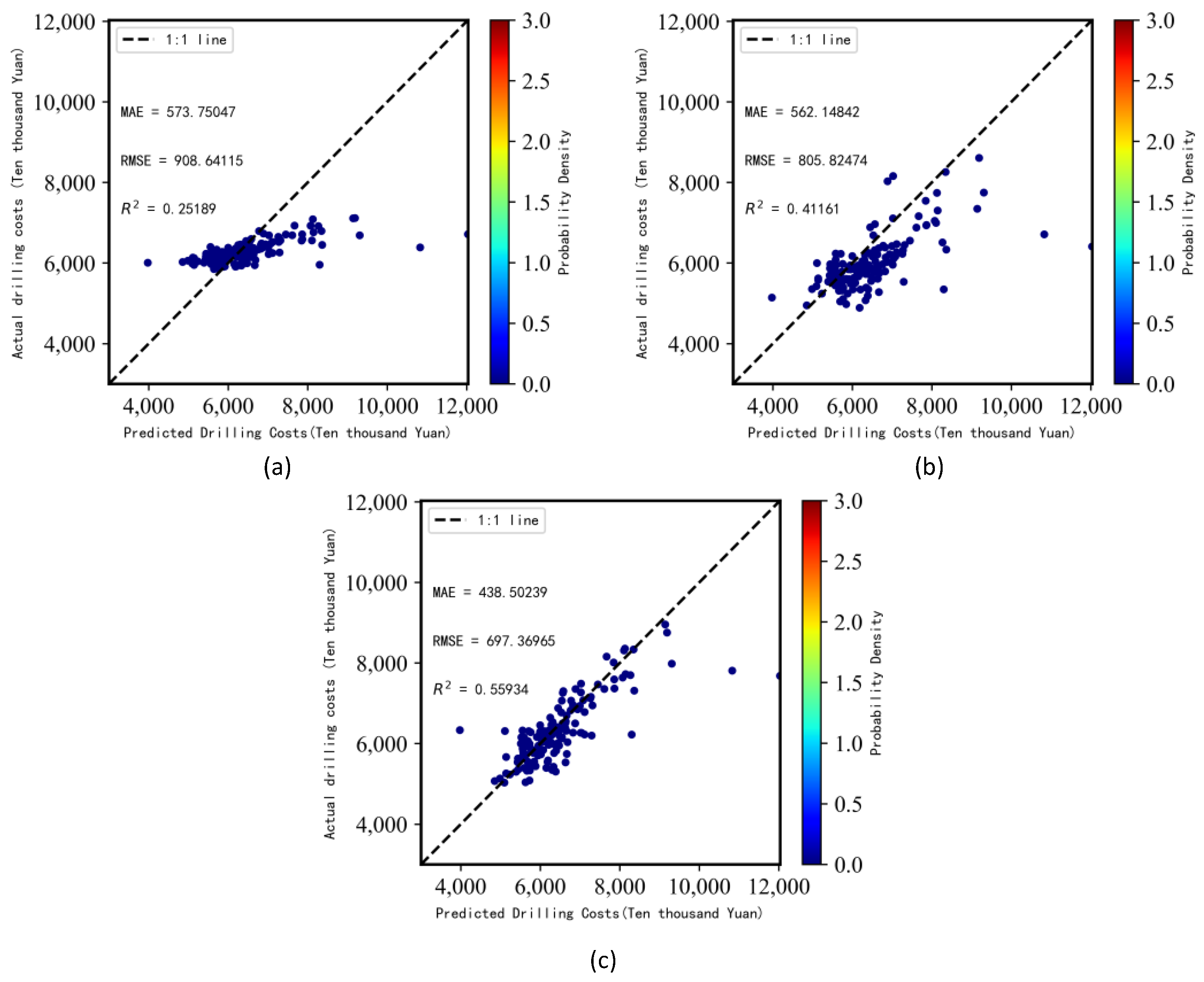
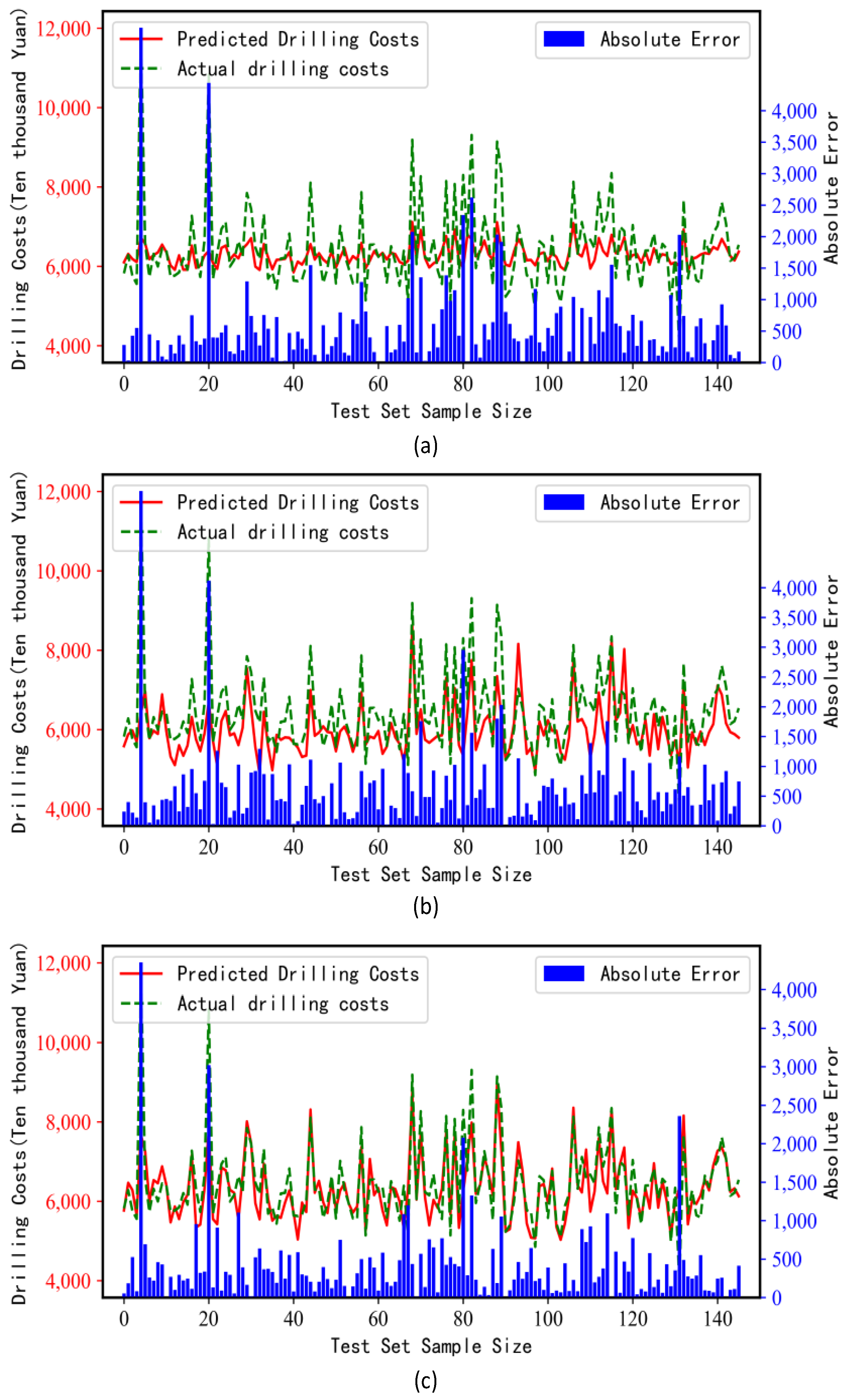
4.8.1. Comparison of Prediction Accuracy

As shown in Figure 5, these are the results of the predictive evaluation metrics for the SVM model, the LSTM model and the LSTM_SVM_Stacking model. The Stacking model has the lowest RMSE (697.37), which is about 22% lower than the single model. The LSTM (854.53) is slightly better than the SVM (908.64), but the difference is not significant. The Stacking model significantly outperforms the single model in terms of overall prediction accuracy. The Stacking model has the lowest MAE (438.50), which is about 20.62% lower than the single model. The MAEs of SVM (573.75) and LSTM (552.38) are very close to each other. The trend of improvement in MAE is consistent with the RMSE, indicating consistency of results. The R² value of the Stacking model (0.559) is significantly higher than that of the single model. The LSTM (0.338) is slightly better than the SVM (0.252). The R² of the Stacking model almost doubled, indicating a significant improvement in the explanatory power of the model.

Figure 5. Comparison of RMSE\MAE\R² Values for Three Models.

SVM and LSTM have similar performance, suggesting that they may capture different features in the data. LSTM slightly outperforms SVM, possibly due to the ability to better handle temporal features in the data. The Stacking model significantly outperforms a single model, demonstrating the effectiveness of integrated learning. Performance improvement may come from combining the advantages of different models.

4.8.2. Discussion

Figure 6 illustrates the results of the evaluation of the three models. The probability density plot modelled to predict shale gas cost regressions is shown, providing detailed information on the model predictions.

Figure 6. Three models drilling cost prediction effects. (a) SVM Model, (b) LSTM Model, (c) LSTM_SVM_Stacking Model.

• Characteristic Analysis of the Prediction Distribution

When the LSTM_SVM_Stacking model is compared with the SVM model and the LSTM model, its probability density points show obvious centralised distribution characteristics, with a large number of prediction points clustered around the standard line; moreover, the degree of dispersion of the predicted values is small, indicating that the prediction results of the model have a high degree of stability, coupled with the symmetry of the distribution pattern of the predicted values, which means that the prediction errors of the model are more balanced in the positive and negative directions. This concentrated distribution indicates that the shale gas cost prediction model has achieved excellent results in this task and is able to accurately capture the correlation between the true value and the predicted value.

2.

Analysis of prediction accuracy:

Further examination of the predicted probability density plots shows that there is a close correlation between the predicted and true values. The LSTM_SVM_Stacking model’s close fit of the predicted points to the standard line compared to the SVM model and the LSTM model reflects the model’s high prediction accuracy. In addition, the LSTM_SVM_Stacking model has fewer outliers and outliers, indicating that the model maintains stable prediction performance for different input scenarios with good confidence. This close relationship indicates that the model has high prediction accuracy and reliability for the problem under study.

To ensure the model’s ability to predict shale gas costs for unknown samples, shale gas drilling cost prediction curves were generated on the test set, as shown in Figure 3 and Figure 4. As can be seen in Figure 7, the SVM model, the LSTM model and the LSTM_SVM_Stacking model were used to predict the drilling costs on the test set, and the predicted curves of the LSTM_SVM_Stacking model are basically the same as the actual value curves, which indicates that this study achieves better shale gas drilling cost modelling. In the subsequent shale gas drilling cost prediction, the drilling cost can be simulated with the model of this study on the previously unexamined data, so as to reduce the economic losses caused by the shale gas exploration process.

Figure 7. Three models fitting effects. (a) SVM Model, (b) LSTM Model, (c) LSTM_SVM_Stacking Model.

In addition, this study adopts a stacked integrated learning model of SVM and LSTM, and combines these two models to predictively model the shale gas drilling cost dataset using SVM’s sensitivity to spatial data and LSTM’s sensitivity to temporal features. By exploiting the respective advantages of SVM and LSTM, this study was able to provide a more comprehensive analysis of the various factors in the dataset, resulting in more accurate predictions. The combined model achieved satisfactory prediction results. The Mean Absolute Error (MAE) is 438.50 and the Root Mean Square Error (RMSE) is 697.37, indicating that the model in this study is able to effectively and accurately predict shale gas drilling costs. This indicates that the model used in this study is able to utilise both spatial and temporal information, thus capturing the essential characteristics of drilling costs and improving the accuracy and reliability of the prediction. In order to present the prediction results in a more intuitive manner, this study conducted a visualisation analysis to clearly demonstrate the relationship between the predicted values and the actual values through graphs and charts, thus revealing a certain degree of fit patterns captured by the model. This further validates the validity and reliability of the shale gas drilling cost prediction model used in this study. The results of this study provide a reliable and effective methodology for predicting shale gas drilling costs, providing targeted guidance for policy makers and practitioners. This will help researchers and policy makers understand the impact of different factors on costs and provide a scientific basis for optimising the drilling process and controlling costs. The results of this study are a valuable contribution to the field of cost optimisation in the shale gas industry, in line with the goal of sustainable development. In the future, this study will continue to improve the model and refine the dataset by introducing more factors and techniques to increase the accuracy and usefulness of the predictions.

4.9. Economic Analysis of Investment in Selected Drilling Wells in the Changning Block

The Changning Block is located at the southern edge of Sichuan Province, with an east–west length of about 90 km and a north–south width of about 49 km, in the hinterland of Yibin City, as shown in Figure 8. Tectonically, the Changning block belongs to the Sichuan–Guizhou combination at the western edge of the Yangzi plate and is under the joint control of the tectonic development of the southwest Loushan fold belt outside the basin and the southern Sichuan low fold belt inside the basin. The Changning area has undergone many periods of tectonic movements of varying intensities, among which the orogenic movements since the Yanshan period have resulted in the development of a series of fold deformations and fractures in the area. The Changning backslope is a large-scale fold deformation structure under the complex tectonic background and. due to the different tectonic stresses, different parts of the backslope also show obvious differences. The two wings of the backslope show obvious asymmetric features, with the south and west wings being gentler and the north and east wings being steeper. Under extrusion stress, the Changning backslope develops a series of backslope-related fractures, which are mainly small-scale reverse faults. Compared with the stable area in the basin, the Wufeng–Longmaxi formation in this area is relatively shallow in depth, with a high degree of fracture and fold development, and the local favourable tectonic development sites in the context of tectonic activities are the main targets for shale gas exploration.

Figure 8. Location of the Changning Block.

The rapid urbanisation in recent years has led to an increasing demand for natural gas supply. In order to meet the natural gas production targets and capacity building requirements in Sichuan Province, the expeditious construction and implementation of the Changning H3 Test Mine Gas Collection and Transmission Project has become imperative. This project has significant implications for enhancing clean energy supply, optimising economic benefits for enterprises and facilitating socio-economic development. It also contributes to the transformation of the regional energy structure and atmospheric environmental quality through the increased utilisation of clean energy resources.

Based on comprehensive geological assessments, including reservoir conditions, tectonic fracture characteristics, drilling result analysis and surface topographic evaluation of the Longmaxi Formation shale in the Ning 201 and Ning 209 well areas, 20 shale gas wells (e.g., Ning 209H70-3) have been successfully completed in the Changning Block. These wells serve as analysis and verification objects for shale gas exploration and development.

The analysis results shown in Figure 9 indicate that the prediction model has satisfactory overall performance, achieving a Mean Absolute Percentage Error (MAPE) of 6.41%. The model shows optimal accuracy in predicting medium investment ranges (60–70 million yuan), with a correlation coefficient of 0.73, indicating robust tracking of actual value trends. However, several limitations were identified: (1) reduced ability to predict extreme values, especially in the lower range; (2) reduced amplitude of predicted value fluctuations compared to actual values; (3) delayed response to abrupt changes; and (4) reduced prediction accuracy in extreme scenarios, suggesting a tendency to underestimate risk. Nevertheless, the model retains reliable utility within median ranges, where predictive risk remains minimal.

Figure 9. Comparison of actual and predicted investment in selected drilling wells in the Changning block.

5. Conclusions

In this study, by constructing a comprehensive shale gas drilling cost database covering spatio-temporal dimensions, we identified the key cost influencing factors by applying the Gradient Boosted Decision Tree (GBDT) model, and innovatively proposed a stacked integrated learning framework based on SVM and LSTM. The model significantly improves the accuracy of cost prediction, and the coefficient of determination (R²) is improved from 0.25189 (SVM) and 0.33834 (LSTM) of the traditional single model to 0.55934. The research results not only enrich the research methodology in the field of energy economics and provide a new technical way for the cost management of shale gas drilling, but also provide an operable technical support for the cost management practice of the oil and gas industry. The follow-up research will further expand the data dimension and optimise the model structure to improve the adaptability and reliability of the prediction model under different regional conditions, so as to promote the economic and sustainable development of shale gas resources.

References

1. Tariq, Z.; Aljawad, M.S.; Hasan, A.; Murtaza, M.; Mohammed, E.; El-Husseiny, A.; Alarifi, S.A.; Mahmoud, M.; Abdulraheem, A. A systematic review of data science and machine learning applications to the oil and gas industry. J. Pet. Explor. Prod. Technol. 2021, 11, 4339–4374. [Google Scholar] [CrossRef]
2. Nikolaou, M. Computer-aided process engineering in oil and gas production. Comput. Chem. Eng. 2013, 51, 96–101. [Google Scholar] [CrossRef]
3. Gao, J.; You, F. Design and optimization of shale gas energy systems: Overview, research challenges, and future directions. Comput. Chem. Eng. 2017, 106, 699–718. [Google Scholar] [CrossRef]
4. Lashari, S.e.Z.; Takbiri-Borujeni, A.; Fathi, E.; Sun, T.; Rahmani, R.; Khazaeli, M. Drilling performance monitoring and optimization: A data-driven approach. J. Pet. Explor. Prod. Technol. 2019, 9, 2747–2756. [Google Scholar] [CrossRef]
5. Nautiyal, A.; Mishra, A.K. Machine Learning Application in Enhancing Drilling Performance. Procedia Comput. Sci. 2023, 218, 877–886. [Google Scholar] [CrossRef]
6. Goodkey, B.; Carvalho, R.; Davila, A.N.; Hernandez, G.; Corona, M.; Atriby, K.; Herrera, C. Recipe for digital change: A case study approach to drilling automation. In Proceedings of the SPE/IADC Middle East Drilling Technology Conference and Exhibition, Abu Dhabi, United Arab Emirates, 27–29 May 2021. [Google Scholar] [CrossRef]
7. Yuan, S.; Han, H.; Wang, H.; Luo, J.; Wang, Q.; Lei, Z.; Xi, C.; Li, J. Research progress and potential of new enhanced oil recovery methods in oilfield development. Pet. Explor. Dev. 2024, 51, 963–980. [Google Scholar] [CrossRef]
8. Liu, H.; Ren, Y.; Li, X.; Deng, Y.; Wang, Y.; Cao, Q.; DU, J.; Lin, Z.; Wang, W. Research status and application of artificial intelligence large models in the oil and gas industry. Pet. Explor. Dev. 2024, 51, 1049–1065. [Google Scholar] [CrossRef]
9. Hegde, C.; Gray, K. Use of machine learning and data analytics to increase drilling efficiency for nearby wells. J. Nat. Gas Sci. Eng. 2017, 40, 327–335. [Google Scholar] [CrossRef]
10. Sajadfar, N.; Ma, Y. A hybrid cost estimation framework based on feature-oriented data mining approach. Adv. Eng. Inform. 2015, 29, 633–647. [Google Scholar] [CrossRef]
11. Barbosa, L.F.F.M.; Nascimento, A.; Mathias, M.H.; de Carvalho, J.A., Jr. Machine learning methods applied to drilling rate of penetration prediction and optimization—A review. J. Pet. Sci. Eng. 2019, 183, 106332. [Google Scholar] [CrossRef]
12. Ren, J.; Jiang, J.; Zhou, C.; Li, Q.; Xu, Z. Research on adaptive feature optimization and drilling rate prediction based on real-time data. Geoenergy Sci. Eng. 2024, 242, 213247. [Google Scholar] [CrossRef]
13. Eskandarian, S.; Bahrami, P.; Kazemi, P. A comprehensive data mining approach to estimate the rate of penetration: Application of neural network, rule based models and feature ranking. J. Pet. Sci. Eng. 2017, 156, 605–615. [Google Scholar] [CrossRef]
14. Pan, H.; Cheng, G.; Ding, J. Drilling Cost Prediction Based on Self-adaptive Differential Evolution and Support Vector Regression. In Intelligent Data Engineering and Automated Learning—IDEAL 2013; Yin, H., Tang, K., Gao, Y., Klawonn, F., Lee, M., Weise, T., Li, B., Yao, X., Eds.; Springer: Berlin/Heidelberg, Germany, 2013; pp. 67–75. [Google Scholar] [CrossRef]
15. Sircar, A.; Yadav, K.; Rayavarapu, K.; Bist, N.; Oza, H. Application of machine learning and artificial intelligence in oil and gas industry. Pet. Res. 2021, 6, 379–391. [Google Scholar] [CrossRef]
16. Polikar, R. Ensemble Learning. In Ensemble Machine Learning; Zhang, C., Ma, Y., Eds.; Springer: New York, NY, USA, 2012. [Google Scholar] [CrossRef]
17. Xu, W.; Zhu, Y.; Wei, Y.; Su, Y.; Xu, Y.; Ji, H.; Liu, D. Prediction Model of Drilling Costs for Ultra-Deep Wells Based on GA-BP Neural Network. Energy Eng. 2023, 120, 1701–1715. [Google Scholar] [CrossRef]
18. Liu, N.; Gao, H.; Zhao, Z.; Hu, Y.; Duan, L. A stacked generalization ensemble model for optimization and prediction of the gas well rate of penetration: A case study in Xinjiang. J. Pet. Explor. Prod. Technol. 2022, 12, 1595–1608. [Google Scholar] [CrossRef]
19. Yehia, T.; Gasser, M.; Ebaid, H.; Meehan, N.; Okoroafor, E.R. Comparative analysis of machine learning techniques for predicting drilling rate of penetration (ROP) in geothermal wells: A case study of FORGE site. Geothermics 2024, 121, 103028. [Google Scholar] [CrossRef]
20. Nautiyal, A.; Mishra, A.K. Drilling efficiency enhancement in oil and gas domain using machine learning. Int. J. Oil Gas Coal Technol. 2023, 32, 121–143. [Google Scholar] [CrossRef]
21. Matinkia, M.; Sheykhinasab, A.; Shojaei, S.; Vojdani Tazeh Kand, A.; Elmi, A.; Bajolvand, M.; Mehrad, M. Developing a New Model for Drilling Rate of Penetration Prediction Using Convolutional Neural Network. Arab. J. Sci. Eng. 2022, 47, 11953–11985. [Google Scholar] [CrossRef]
22. Tewari, S.; Dwivedi, U.D.; Biswas, S. Intelligent Drilling of Oil and Gas Wells Using Response Surface Methodology and Artificial Bee Colony. Sustainability 2021, 13, 1664. [Google Scholar] [CrossRef]
23. Eltrissi, M.; Yousef, O.; El-Banbi, A.; Khalaf, F. Drilling operation optimization using machine learning framework. Geoenergy Sci. Eng. 2023, 228, 211969. [Google Scholar] [CrossRef]
24. Yang, Z.; Liu, Y.; Qin, X.; Dou, Z.; Yang, G.; Lv, J.; Hu, Y. Optimization of Drilling Parameters of Target Wells Based on Machine Learning and Data Analysis. Arab. J. Sci. Eng. 2023, 48, 9069–9084. [Google Scholar] [CrossRef]
25. Elahifar, B.; Hosseini, E. Automated real-time prediction of geological formation tops during drilling operations: An applied machine learning solution for the Norwegian Continental Shelf. J. Petrol. Explor. Prod. Technol. 2024, 14, 1661–1703. [Google Scholar] [CrossRef]
26. Sabah, M.; Talebkeikhah, M.; Wood, D.A.; Khosravanian, R.; Anemangely, M.; Younesi, A. A machine learning approach to predict drilling rate using petrophysical and mud logging data. Earth Sci. Inform. 2019, 12, 319–339. [Google Scholar] [CrossRef]
27. Li, G.; Lu, W.; Song, X.; Tian, S.; Zhu, Z. Intelligent Drilling and Completion: A Review. Engineering 2022, 18, 33–48. [Google Scholar] [CrossRef]
28. Yang, X.Y.; Cui, M.; Zhang, Y.L.; Jing, L.Z.; Ji, Y.; Shi, X.Y. Optimized Drilling Status Recognition for Oil Drilling Using Artificial Intelligence: Empirical Research and Methodology. In Proceedings of the International Field Exploration and Development Conference 2023; Springer Series in Geomechanics and Geoengineering. Lin, J., Ed.; Springer: Singapore, 2023. [Google Scholar] [CrossRef]
29. Bello, O.; Holzmann, J.; Yaqoob, T.; Teodoriu, C. Application of Artificial Intelligence Methods In Drilling System Design And Operations: A Review Of The State Of The Art. J. Artif. Intell. Soft Comput. Res. 2015, 5, 121–139. [Google Scholar] [CrossRef]
30. Gan, C.; Cao, W.; Liu, K. To Improve Drilling Efficiency by Multi-objective Optimization of Operational Drilling Parameters in the Complex Geological Drilling Process. In Proceedings of the 2018 37th Chinese Control Conference (CCC), Wuhan, China, 25–27 July 2018; pp. 10238–10243. [Google Scholar] [CrossRef]
31. Ozdemir, A.; Güllü, A.; Yaşar, E.; Palabiyik, Y. Drilling Engineering Assessment and Cost Analysis of Oil and Gas Wells Drilled in Onshore of Turkey. Int. J. Earth Sci. Knowl. Appl. 2021, 3, 235–243. [Google Scholar]
32. Nwanwe, O.; Teodoriu, C. Matrix selection and comparison for selecting drilling methods and technologies for a wide range of applications. J. Pet. Sci. Eng. 2020, 192, 107289. [Google Scholar] [CrossRef]
33. Purba, D.; Adityatama, D.W.; Agustino, V.; Fininda, F.; Alamsyah, D.; Muhammad, F. Geothermal Drilling Cost Optimization in Indonesia: A Discussion of Various Factors. In Proceedings of the 45th Workshop on Geothermal Reservoir Engineering Stanford University (SGP-TR-216), Stanford, CA, USA, 10–12 February 2020. [Google Scholar]
34. Mustafa, A.B.; Abbas, A.K.; Alsaba, M.; Alameen, M. Improving drilling performance through optimizing controllable drilling parameters. J. Pet. Explor. Prod. Technol. 2021, 11, 1223–1232. [Google Scholar] [CrossRef]
35. Mistré, M.; Crénes, M.; Hafner, M. Shale gas production costs: Historical developments and outlook. Energy Strat. Rev. 2018, 20, 20–25. [Google Scholar] [CrossRef]
36. Zou, C.; Dong, D.; Wang, Y.; Li, X.; Huang, J.; Wang, S.; Guan, Q.; Zhang, C.; Wang, H.; Liu, H.; et al. Shale gas in China: Characteristics, challenges and prospects (II). Pet. Explor. Dev. 2016, 43, 182–196. [Google Scholar] [CrossRef]
37. Wang, Q.; Li, R. Research status of shale gas: A review. Renew. Sustain. Energy Rev. 2017, 74, 715–720. [Google Scholar] [CrossRef]
38. Yuan, J.; Luo, D.; Feng, L. A review of the technical and economic evaluation techniques for shale gas development. Appl. Energy 2015, 148, 49–65. [Google Scholar] [CrossRef]
39. Curtis, J.; John, B. Fractured Shale-Gas Systems. AAPG Bull. 2002, 86, 1921–1938. [Google Scholar] [CrossRef]
40. Friedman, J.H. Greedy function approximation: A gradient boosting machine. Ann. Stat. 2001, 29, 1189–1232. [Google Scholar] [CrossRef]
41. Chen, T.; Guestrin, C. XGBoost: A Scalable Tree Boosting System. In Proceedings of the 22nd ACM SIGKDD International Conference on Knowledge Discovery and Data Mining, San Francisco, CA, USA, 13–17 August 2016; ACM: New York, NY, USA, 2016; pp. 785–794. [Google Scholar] [CrossRef]
42. Alonso-Español, A.; Bravo, E.; Ribeiro-Vidal, H.; Virto, L.; Herrera, D.; Alonso, B.; Sanz, M. The Antimicrobial Activity of Curcumin and Xanthohumol on Bacterial Biofilms Developed over Dental Implant Surfaces. Int. J. Mol. Sci. 2023, 24, 2335. [Google Scholar] [CrossRef] [PubMed]
43. Cortes, C.; Vapnik, V. Support-Vector Networks. Mach. Learn. 1995, 20, 273–297. [Google Scholar] [CrossRef]
44. Vapnik, V.N. Statistical Learning Theory; Wiley-Interscience: New York, NY, USA, 1998. [Google Scholar]
45. Smola, A.J.; Schölkopf, B. A tutorial on support vector regression. Stat. Comput. 2004, 14, 199–222. [Google Scholar] [CrossRef]
46. Hochreiter, S.; Schmidhuber, J. Long short-term memory. Neural Comput. 1997, 9, 1735–1780. [Google Scholar] [CrossRef] [PubMed]
47. Gers, F.A.; Schmidhuber, J.; Cummins, F. Learning to forget: Continual prediction with LSTM. In Proceedings of the 1999 Ninth International Conference on Artificial Neural Networks ICANN 99 (Conf. Publ. No. 470), Edinburgh, UK, 7–10 September 1999; Volume 2, pp. 850–855. [Google Scholar] [CrossRef]
48. Greff, K.; Srivastava, R.K.; Koutník, J.; Steunebrink, B.R.; Schmidhuber, J. LSTM: A Search Space Odyssey. IEEE Trans. Neural Netw. Learn. Syst. 2017, 28, 2222–2232. [Google Scholar] [CrossRef]
49. He, J.; Li, K.; Wang, X.; Gao, N.; Mao, X.; Jia, L. A Machine Learning Methodology for Predicting Geothermal Heat Flow in the Bohai Bay Basin, China. Nat. Resour. Res. 2022, 31, 237–260. [Google Scholar] [CrossRef]
50. Bergstra, J.; Bengio, Y. Random Search for Hyper-Parameter Optimization. J. Mach. Learn. Res. 2012, 13, 281–305. [Google Scholar]
51. Ron, K. A study of cross-validation and bootstrap for accuracy estimation and model selection. In Proceedings of the 14th International Joint Conference on Artificial Intelligence—Volume 2 (IJCAI’95), Montreal, QC, Canada, 20–25 August 1995; Morgan Kaufmann Publishers Inc.: San Francisco, CA, USA, 1995; pp. 1137–1143. [Google Scholar]
52. Chai, T.; Draxler, R.R. Root Mean Square Error (RMSE) or Mean Absolute Error (MAE)?—Arguments against Avoiding RMSE in the Literature. Geosci. Model Dev. 2014, 7, 1247–1250. [Google Scholar] [CrossRef]
53. Hastie, T.; Tibshirani, R.; Friedman, J. The Elements of Statistical Learning: Data Mining, Inference, and Prediction; Springer Science & Business Media: New York, NY, USA, 2009. [Google Scholar] [CrossRef]
Disclaimer/Publisher’s Note: The statements, opinions and data contained in all publications are solely those of the individual author(s) and contributor(s) and not of MDPI and/or the editor(s). MDPI and/or the editor(s) disclaim responsibility for any injury to people or property resulting from any ideas, methods, instructions or products referred to in the content.
Article Metrics
Citations
Article Access Statistics
Multiple requests from the same IP address are counted as one view.