Coupled Elastic–Plastic Damage Modeling of Rock Based on Irreversible Thermodynamics

Abstract

Shale is a common rock in oil and gas extraction, and the study of its nonlinear mechanical behavior is crucial for the development of engineering techniques such as hydraulic fracturing. This paper establishes a new coupled elastic–plastic damage model based on the second law of thermodynamics, the strain equivalence principle, the non-associated flow rule, and the Drucker–Prager yield criterion. This model is used to describe the mechanical behavior of shale before and after peak strength and has been implemented in ABAQUS via UMAT for numerical computation. The model comprehensively considers the quasi-brittle and anisotropic characteristics of shale, as well as the strength degradation caused by damage during both the elastic and plastic phases. A damage yield function has been established as a criterion for damage occurrence, and the constitutive integration algorithm has been derived using a regression mapping algorithm. Compared with experimental data from La Biche shale in Canada, the theoretical model accurately simulated the stress–strain curves and volumetric–axial strain curves of shale under confining pressures of 5 MPa, 25 MPa, and 50 MPa. When compared with experimental data from shale in Western Hubei and Eastern Chongqing, China, the model precisely fitted the stress–strain curves of shale at pressures of 30 MPa, 50 MPa, and 70 MPa, and at bedding angles of 0°, 22.5°, 45°, and 90°. This proves that the model can effectively predict the failure behavior of shale under different confining pressures and bedding angles. Additionally, a sensitivity analysis has been performed on parameters such as the plastic hardening rate b, damage evolution rate B_ω, weighting factor r, and damage softening parameter a. This research is expected to provide theoretical support for the efficient extraction technologies of shale oil and gas.

1. Introduction

As global energy demands continue to rise, conventional oil and gas resources are gradually depleting. Unconventional resources, exemplified by shale gas and shale oil, are increasingly becoming a significant component of the energy structure [1,2,3,4]. According to reports by the U.S. Energy Information Administration and the International Energy Agency, the global known reserves of shale gas are approximately 7299 trillion cubic feet, with proven shale oil reserves amounting to 345 billion barrels [5,6]. These resources are primarily located in the United States, China, Russia, Australia, and Canada (Figure 1). Rational and efficient development and utilization of these shale oil and gas resources can enhance national energy self-sufficiency and stability, accelerate the adjustment of the global energy landscape, and achieve energy diversification and sustainable development [7,8,9,10,11]. However, the efficient and safe extraction of oil and gas from shale still poses challenges. Unlike common granite or sandstone, shale is a typical sedimentary rock. Its naturally formed bedding planes during sedimentation give it typical heterogeneity and anisotropy at different scales, significantly affecting the shale’s strength characteristics, deformation behavior, and failure modes [12,13,14,15,16]. Additionally, the inherent plastic deformation and damage behavior of shale also impact the extraction of shale oil and gas [17,18,19]. Therefore, correctly understanding the stress–strain behavior of shale and establishing appropriate constitutive models to explain, describe, and predict the plastic and damage laws of shale is crucial for the development of shale oil and gas extraction technologies such as hydraulic fracturing, the stability of wellbore, and core issues such as energy production.

Quasi-brittleness and anisotropy are two characteristics of shale. On one hand, shale exhibits quasi-brittleness [20,21,22]. Under compressive stress, quasi-brittle geomaterials exhibit inelastic deformation, including degradation of elastic stiffness, strain hardening or softening, and confinement dependency. The stress–strain curve of shale initially shows linear elastic deformation, followed by nonlinear deformation due to the accumulation of minor plastic strains caused by microcrack initiation, crack propagation, and coalescence [17,23,24,25]. After reaching peak stress, shale enters a strain-softening phase where crack accumulation is significant, and irreversible strain markedly increases. The failure behavior in quasi-brittle rocks includes plastic effects; at the mesoscale, the failure process in shale can be understood as two physical phenomena: one is damage behavior caused by microcrack propagation, and the other is macroscopic irreversible strain caused by frictional sliding along crack surfaces, i.e., elastoplastic mechanical behavior [26,27,28,29,30,31]. These behaviors have an intrinsic coupling during the failure process of shale, where the accumulation of frictional sliding leads to an increase in microcracks, which in turn enhances frictional sliding, meaning damage evolution and plastic flow are intrinsically coupled [32,33,34,35,36,37,38]. Therefore, the mechanical behavior of shale should be described using a damage model coupled with plasticity theory.

On the other hand, shale exhibits anisotropy. Many experimental studies have shown that the mechanical behavior of rocks has strong anisotropy [39,40,41,42,43,44,45,46,47,48]. Anisotropic constitutive models are inherently complex; to simplify theoretical calculations, previous scholars mostly considered rock materials as isotropic [49,50,51,52,53,54,55]. However, the strength and deformation characteristics of shale vary significantly under different loading directions, and ignoring anisotropy would cause models to inaccurately simulate and predict the bearing capacity, stability, and stress-strain laws of shale in actual conditions. Therefore, the anisotropy of shale must be fully considered.

The failure mechanisms in rock mechanics are multifaceted, including but not limited to microcrack slippage, micropore fragmentation, elastic failure of mineral particles, crystal dislocation movement, crack growth speed and direction, and clustering effects between cracks or pores [56,57,58,59,60,61,62]. These mechanisms are both the root causes of rock damage and reasons for energy dissipation. Previous studies have proposed two types of quasi-brittle rock elastoplastic damage coupling models. One is based on micromechanics approaches [63,64,65,66], which consider the behavior of cracks in detail but lead to complex formulations that are often difficult to compute or apply practically. The other is based on continuous damage models, usually grounded in irreversible thermodynamics, analyzing rock damage mechanisms from the perspective of energy dissipation [67,68,69,70,71]. The resulting constitutive equations comply with the fundamental laws of thermodynamics [51,72,73,74,75,76] and effectively characterize the irreversible energy dissipation processes and the thermodynamic state of the material system, grounded in deep thermodynamic principles and rigorous theoretical bases [77,78,79,80]. Thus, determining the quantitative relationship between energy dissipation and damage variables is key to establishing a thermodynamic constitutive model.

Previous research has helped understand the mechanical properties of shale under various conditions, essential for optimizing drilling technology, ensuring wellbore stability, and enhancing the efficiency and safety of shale oil and gas extraction. However, current research on shale constitutive models still faces some limitations. (1) Few studies on shale constitutive models within the framework of thermodynamics, leading to models that do not adequately express the irreversible energy dissipation processes in shale materials. (2) Existing models often only consider parts of shale’s quasi-brittleness, anisotropy, and thermodynamic principles, lacking a comprehensive theoretical model. (3) The mechanical behavior of shale should be described using damage models coupled with plasticity theory. (4) Some elastoplastic damage coupling models for shale are too complex for calculation or practical application. (5) The understanding of constitutive model parameters is still insufficient, requiring further discussion and summary of model parameter sensitivity.

This paper integrates elastoplastic models and theories related to irreversible thermodynamics to construct a shale elastoplastic damage coupling constitutive model. An anisotropy parameter related to loading direction is introduced to reflect the direction dependency and anisotropy of shale’s mechanical behavior. Through UMAT subroutine programming, it has been applied within the ABAQUS 2022. The model’s validity is verified by simulating the stress–strain curves of La Biche shale and Eastern Yunnan–Western Chongqing shale experiments. The analysis of four model parameters on residual strength, elastic damage, plastic damage, peak strength, and damage softening, among others, was conducted.

2. Basic Framework of the Elastoplastic Damage Coupled Model

2.1. Thermodynamic Framework

From the perspective of macroscopic continuum mechanics, the occurrence of damage in shale is always accompanied by energy dissipation. This process must comply with the laws of irreversible thermodynamics. According to the principle of energy conservation, the equation can be written as:

$$\dot{K}+\dot{E}=W+q$$

(1)

where K is kinetic energy; E is internal energy; W is the work done by external forces; q is the rate of change of internal energy.

Expanding the expression for kinetic energy:

$$K={\displaystyle \frac{1}{2}}{\displaystyle {\int }_{\mathsf{\Omega }}\rho }\dot{u}\cdot \dot{u}d\mathsf{\Omega }$$

(2)

where ρ is material density; u is the rate of displacement change; Ω is the volume of the material.

Taking the time derivative of K, we obtain the rate of change of kinetic energy:

$$\dot{K}={\displaystyle \frac{d}{dt}}\left({\displaystyle \frac{1}{2}}{\displaystyle {\int }_{\mathsf{\Omega }}\rho }\dot{u}\cdot \dot{u}d\mathsf{\Omega }\right)={\displaystyle \frac{1}{2}}{\displaystyle {\int }_{\mathsf{\Omega }}\rho }\dot{u}\cdot \ddot{u}d\mathsf{\Omega }$$

(3)

where $\ddot{u}$ is the acceleration of the material.

From the equilibrium equation of elasticity:

$$\rho \ddot{u}=\nabla \cdot \sigma +\rho b$$

(4)

Substituting Equation (4) into Equation (3), we obtain the expansion for the rate of change of kinetic energy:

$$\begin{array}{l}\dot{K}={\displaystyle {\int }_{\mathsf{\Omega }}\rho }\dot{u}\cdot (\nabla \cdot \sigma +\rho b)d\mathsf{\Omega }={\displaystyle {\int }_{\mathsf{\Omega }}\nabla }\cdot \sigma \cdot \dot{u}d\mathsf{\Omega }+{\displaystyle {\int }_{\mathsf{\Omega }}\rho }\dot{u}\cdot bd\mathsf{\Omega }\hfill \\ ={\displaystyle {\int }_{\mathsf{\Delta }\mathsf{\Omega }}\sigma }\cdot n\cdot \dot{u}dS-{\displaystyle {\int }_{\mathsf{\Omega }}\sigma }:(\nabla \dot{u})d\mathsf{\Omega }+{\displaystyle {\int }_{\mathsf{\Omega }}\rho }\dot{u}\cdot bd\mathsf{\Omega }\hfill \\ ={\displaystyle {\int }_{\mathsf{\Omega }\mathsf{\Omega }}t}\cdot \dot{u}dS-{\displaystyle {\int }_{\mathsf{\Omega }}\sigma }:\dot{\epsilon }d\mathsf{\Omega }+{\displaystyle {\int }_{\mathsf{\Omega }}\rho }\dot{u}\cdot bd\mathsf{\Omega }\hfill \end{array}$$

(5)

The expansions for internal energy E, external work W, and the rate of change of internal energy q are as follows:

$$E={\displaystyle {\int }_{\mathsf{\Omega }}\rho }ed\mathsf{\Omega }$$

(6)

$$W={\displaystyle {\int }_{\partial \mathsf{\Omega }}t}\cdot \dot{u}dS+{\displaystyle {\int }_{\mathsf{\Omega }}\rho }\dot{u}\cdot bd\mathsf{\Omega }$$

(7)

$$q={\displaystyle \frac{\partial Q}{\partial t}}={\displaystyle {\int }_{\mathsf{\Omega }}\rho }\gamma d\mathsf{\Omega }-{\displaystyle {\int }_{\mathsf{\Omega }}\sigma }:(\nabla \dot{u})d\mathsf{\Omega }$$

(8)

Substituting Equation (5) to Equation (8) into Equation (1), we obtain:

$$\rho \dot{e}=\sigma :\dot{\epsilon }+\rho \gamma -\nabla \cdot h$$

(9)

When only heat exchange with the surroundings occurs without material exchange:

$$\left\{\begin{array}{l}{\displaystyle \frac{dS}{dt}}={\displaystyle \frac{\dot{Q}}{T}}+{\dot{S}}_i\\ {\dot{S}}_i\ge 0\end{array}\right.$$

(10)

Rewriting Equation (10), we obtain the Clausius–Duhem inequality:

$${\displaystyle \frac{dS}{dt}}\ge {\displaystyle \frac{\dot{Q}}{T}}$$

(11)

The integral form of Equation (11):

$${\displaystyle {\int }_{\mathsf{\Omega }}\rho }\dot{s}d\mathsf{\Omega }\ge {\displaystyle {\int }_{\mathsf{\Omega }}\frac{\rho \gamma }{T}}d\mathsf{\Omega }-{\displaystyle {\int }_{\partial \mathsf{\Omega }}\frac{h\cdot n}{T}}dS$$

(12)

Based on the divergence theorem, this equation is transformed to:

$${\displaystyle {\int }_{\mathsf{\Omega }}\rho }\dot{s}d\mathsf{\Omega }\ge {\displaystyle {\int }_{\mathsf{\Omega }}\frac{\rho \gamma }{T}}d\mathsf{\Omega }-{\displaystyle {\int }_{\mathsf{\Omega }}\left(\frac{\nabla \cdot h}{T}-\frac{h}{T^2}\cdot \nabla T\right)}d\mathsf{\Omega }$$

(13)

$${\displaystyle {\int }_{\mathsf{\Omega }}\left(\rho \dot{s}-\frac{\rho \gamma }{T}+\frac{\nabla \cdot h}{T}-\frac{h}{T^2}\cdot \nabla T\right)}d\mathsf{\Omega }\ge 0$$

(14)

Since Equation (14) holds under any arbitrary volume and the absolute temperature is always non-negative, removing the integral sign and rearranging:

$$\rho T\dot{s}-(\rho \gamma -\nabla \cdot h)-{\displaystyle \frac{h}{T}}\cdot \nabla T\ge 0$$

(15)

Combining Equation (9) and Equation (9), the arrangement yields:

$$\sigma :\dot{\epsilon }-\rho (\dot{e}-T\dot{s})\ge 0$$

(16)

Helmholtz free energy can be defined as:

$$\varphi =\rho e-\rho Ts$$

(17)

At this point, the final form of the Clausius–Duhem inequality is:

$$\sigma :\dot{\epsilon }-\dot{\varphi }\ge 0$$

(18)

where σ is the stress tensor; ‘:’ is the double dot product operation between two tensors.

2.2. Stress–Strain Relationship

In the derivation process of the stress–strain relationship for shale, derivation with respect to different parameters is involved. Therefore, in this section, using d and ∂ to denote derivatives is more appropriate. Equation (18) is rewritten as:

$$\sigma :d\epsilon -d\varphi \ge 0$$

(19)

Shale is a quasi-brittle rock, and the total strain in quasi-brittle materials is the sum of elastic strain ε^e and plastic strain ε^P, with the total strain increment being the sum of the increments of elastic dε^e and plastic strains dε^P:

$$\left\{\begin{array}{l}\epsilon ={\epsilon }^e+{\epsilon }^p\\ d\epsilon =d{\epsilon }^e+d{\epsilon }^p\end{array}\right.$$

(20)

According to the principle of strain equivalence, the damage variable can be defined as:

$$\omega =1-E/E_0$$

(21)

where E and E₀ are the elastic moduli of the damaged and undamaged states of the shale, respectively [81].

The thermodynamic potential in rocks can be decomposed into elastic potential energy ${\varphi }^e$ and plastic potential energy ${\varphi }^p$. Under isothermal conditions, the thermodynamic potential in the elastoplastic damage coupling model requires several state variables to describe:

$$\varphi =\varphi \left({\epsilon }^e,{\gamma }^p,\omega \right)={\varphi }^e({\epsilon }^e,\omega )+{\varphi }^p({\gamma }^p,\omega )$$

(22)

where ε^e is the elastic strain; γ^P is the equivalent plastic strain; ω is the damage variable.

Differentiating Equation (22) with respect to time and then substituting it along with Equation (20) into Equation (19), and upon rearrangement, we obtain:

$$(\sigma -{\displaystyle \frac{\partial {\varphi }^e}{\partial {\epsilon }^e}}):d\epsilon +{\displaystyle \frac{\partial {\varphi }^e}{\partial {\epsilon }^e}}:d{\epsilon }^p-{\displaystyle \frac{\partial {\varphi }^p}{\partial {\gamma }^p}}:d{\gamma }^p-{\displaystyle \frac{\partial \varphi }{\partial \omega }}:d\omega \ge 0$$

(23)

The conditions of elastic strain ε^e, equivalent plastic strain γ^P, and damage variable ω as arbitrary values always satisfy Equation (23); hence, we can conclude:

$$\sigma ={\displaystyle \frac{\partial {\varphi }^e}{\partial {\epsilon }^e}}$$

(24)

The thermodynamic forces related to plasticity R and damage Y can be represented as follows:

$$\left\{\begin{array}{l}R=-{\displaystyle \frac{\partial {\varphi }^p}{\partial {\gamma }^p}}\\ Y=-{\displaystyle \frac{\partial \varphi }{\partial \omega }}\end{array}\right.$$

(25)

In the thermodynamic framework, both γ^P and ω are non-negative state variables; therefore, their increments dγ^P and dω are also non-negative during the process of inelastic dissipation, thus satisfying the non-negativity condition expressed in Equation (25). Previous research has shown that the damage-related thermodynamic force Y acts during both the elastic and plastic portions [67,82], allowing Y to be decomposed as follows:

$$Y=r{Y}^e+(1-r)Y^p$$

(26)

where Y^e and Y^P represent the damage-related thermodynamic forces of the elastic and plastic parts, respectively; r is a weighting coefficient controlling the contributions of the elastic and plastic parts. Many triaxial experimental studies with acoustic emission outcomes indicate that damage in quasi-brittle rocks significantly increases after the onset of plasticity, with a greater weight on the plastic component, i.e., the value of the weighting coefficient r ranges from 0 to 0.5 [52,83,84].

According to the non-associated flow rule, plastic potential G^P(σ, γ^P, ω) and damage potential G^ω(Y, ω) are introduced to describe the flow of plastic strain and the evolution of plastic and damage variables:

$$d{\epsilon }^p=d{\lambda }^p{\displaystyle \frac{\partial G^p}{\partial \sigma }}$$

(27)

$$d{\gamma }^p=d{\lambda }^p{\displaystyle \frac{\partial G^p}{\partial R}}$$

(28)

$$d\omega =d{\lambda }^{\omega }{\displaystyle \frac{\partial G^{\omega }}{\partial \sigma }}$$

(29)

where dλ^P and dλ^ω are the increments of the plastic multiplier and damage multiplier, respectively. The yield criterion F^P and the plastic potential G^P do not include R and, thus, can be transformed into γ^P.

The plastic criterion F^P and damage criterion F^ω determine the onset of plastic flow and damage evolution. According to the Kuhn–Tucker conditions, the loading–unloading conditions for plasticity and damage are represented as follows:

$$F^p=0, d{\lambda }^p\ge 0$$

(30)

$$F^{\omega }=0, d{\lambda }^{\omega }\ge 0$$

(31)

During the inelastic loading process, variables σ and Y need to reside on the yield and damage surfaces, as per the consistency condition:

$$d{F}^p={\displaystyle \frac{\partial F^p}{\partial \sigma }}:d\sigma +{\displaystyle \frac{\partial F^p}{\partial {\gamma }^p}}:d{\gamma }^p+{\displaystyle \frac{\partial F^p}{\partial \omega }}:d\omega =0$$

(32)

$$d{F}^{\omega }={\displaystyle \frac{\partial F^{\omega }}{\partial Y^e}}:d{Y}^e+{\displaystyle \frac{\partial F^{\omega }}{\partial Y^p}}:d{Y}^p+{\displaystyle \frac{\partial F^{\omega }}{\partial \omega }}:d\omega =0$$

(33)

The stress–strain relationship shown in Equation (24) lacks an expression for describing the elastic thermodynamic potential ${\varphi }^e$, which can be represented using Hooke’s law for elastic thermodynamic potential [85,86].

$${\varphi }^e({\epsilon }^e,\omega )={\displaystyle \frac{1}{2}}{\epsilon }^e:D:{\epsilon }^e$$

(34)

where D is the function of the damaged elastic stiffness matrix, which is a joint function of the damage variable ω and the elastic stiffness tensor D₀ in the undamaged state. The expression is:

$$D=(1-\omega )D_0$$

(35)

By substituting Equation (34) into Equation (24), the stress–strain relationship can be represented as:

$$\sigma ={\displaystyle \frac{\partial {\varphi }^e}{\partial {\epsilon }^e}}=D:{\epsilon }^e$$

(36)

To better describe the nonlinear behavior of rocks, Equation (36) is written in incremental form:

$$d\sigma =D:d{\epsilon }^e+{\displaystyle \frac{\partial D}{\partial \omega }}:{\epsilon }^{e}d\omega =D:(d\epsilon -d{\epsilon }^p)-D_0:(\epsilon -{\epsilon }^p)d\omega$$

(37)

From Equation (37), it is evident that the stress increments arising from the elastic strain increments and the stress lost due to changes in elastic stiffness constitute the stress increment in the model.

2.3. Elastoplastic Model

The description of the material’s plastic behavior involves combining the yield criterion, flow rule, and hardening function [52,69]. Among these, the Drucker–Prager yield criterion is widely used for shale [14,27,87,88,89,90,91]. However, when dealing with strain hardening and strain softening behavior, traditional yield criteria are no longer suitable. They must be improved and optimized to allow for changes in the yield surface during dilation and contraction. Therefore, the modified yield criterion used in this article is:

$$F^p(\sigma ,{\gamma }^p,\omega )=q+{\alpha }_{1}p-\kappa {\chi }^{p\omega }=0$$

(38)

where q is the equivalent stress, expressed as $q=\sqrt{1.5S:S}$; p is the average stress, expressed as $p=tr(\sigma )/3$; S is the deviatoric stress tensor; α₁ and $\kappa$ are the Drucker–Prager strength parameters, representing internal friction and cohesion, respectively; χ^pω is a function of γ^P, f(θ), and ω, reflecting the impact of plastic hardening, damage softening, and shale bedding angle on the evolution of the yield surface, expressed as:

$${\chi }^{p\omega }=f(\theta )\left[h_1-\left(h_1-h_0\right){\mathrm{e}}^{(-b{\gamma }^p)}\right]{\left(1-\omega \right)}^a$$

(39)

where h₀ and h₁ are the initial and final yield thresholds, respectively; b is the plastic hardening rate, reflecting the rate of hardening. The smaller the value of b, the faster the hardening rate.

Previous research has shown that post-peak strength degradation is related to confinement conditions; thus, it is necessary to introduce the parameter a to describe the influence of confining pressure on damage changes during triaxial experiments [26,59,83]. Moreover, shale and many other rocks exhibit significant directional dependence and anisotropy in mechanical behavior due to their naturally occurring bedding and joint planes [70,92,93,94,95]. To accurately describe this anisotropy caused by differences in bedding plane angles, this study incorporates a function f(θ) related to the bedding plane angle into the yield surface evolution equation (Equation (31)). The magnitude of f(θ) depends on the angle between the stress loading direction and the bedding plane (Figure 2). The specific expressions for parameters a and f(θ) will be provided during the validation phase.

Rock materials exhibit apparent volumetric contraction during triaxial loading [96], and traditionally associated flow rules overlook the energy dissipation and volumetric changes during plastic yielding. Therefore, this article adopts a non-associated flow rule, obtained from:

$$G^p(\sigma ,{\gamma }^p,\omega )=q+{\alpha }_{2}p$$

(40)

where α₂ is a parameter related to shear volume change.

In the elastoplastic loading process without damage evolution, through the non-associated flow rule and consistency condition, it can be obtained:

$$d{\lambda }^p={\displaystyle \frac{\partial F^p}{\partial \sigma }}:D:d\epsilon /H^p$$

(41)

where H^P is the plastic modulus, expressed as:

$$H^p={\displaystyle \frac{\partial F^p}{\partial \sigma }}:D:{\displaystyle \frac{\partial G^p}{\partial \sigma }}-{\displaystyle \frac{\partial F^p}{\partial {\gamma }^p}}\sqrt{{\displaystyle \frac{2}{3}}{\displaystyle \frac{\partial G^p}{\partial S}}:{\displaystyle \frac{\partial G^p}{\partial S}}}$$

(42)

The incremental form of the stress–strain relationship is:

$$d\sigma =D^{ep}:d\epsilon$$

(43)

$$D^{ep}=D-{\displaystyle \frac{1}{H^p}}(D:{\displaystyle \frac{\partial G^p}{\partial \sigma }})\otimes ({\displaystyle \frac{\partial F^p}{\partial \sigma }}:D)$$

(44)

2.4. Elastic Damage Model

The damage criterion is a function of the damage-related thermodynamic force Y. According to statistical damage theory and laboratory data, it has been found that damage evolution follows an exponential function [68,97,98,99]. Therefore, the damage function can be expressed as:

$$F^{\omega }={\omega }_c(1-\exp (B_{\omega }Y))-\omega$$

(45)

where ω_c is the asymptotic damage value during the residual deformation stage; B_ω controls the damage evolution rate.

In the case of elastic damage without plastic flow, one can set F^ω = G^ω, and by the consistency condition:

$$d{\lambda }^{\omega }={\displaystyle \frac{\partial F^{\omega }}{\partial Y^e}}{\epsilon }^e:D_0:d\epsilon /H^{\omega }$$

(46)

$$H^{\omega }={\displaystyle \frac{\partial F^{\omega }}{\partial \omega }}{\displaystyle \frac{\partial G^{\omega }}{\partial Y^e}}$$

(47)

The incremental form of the stress-strain relationship is:

$$\left\{\begin{array}{l}d\sigma =D^{e\omega }:d\epsilon \\ D^{e\omega }=D-{\displaystyle \frac{\partial G^{\omega }}{\partial Y^e}}{\displaystyle \frac{\partial F^{\omega }}{\partial Y^e}}\left(D_0:{\epsilon }^e\right)\otimes \left({\epsilon }^e:D_0\right)/H^{\omega }\end{array}\right.$$

(48)

where D^eω is the fourth-order tensor of elastic damage stiffness.

When only elastic deformation occurs, the damage-related thermodynamic force Y can be obtained from Equations (26) and (34). When plastic deformation occurs, it is necessary to consider the damage-related thermodynamic force Y^P caused by plastic deformation, using the plastic strain increment and the equivalent plastic strain increment to construct the plastic thermodynamic potential ${\varphi }^p$. Given the nonlinear relationship between stress and plastic strain, it is specifically defined as:

$${\varphi }^p({\gamma }^p,\omega )=(1-\omega )\left({\displaystyle {\int }_0^{{\epsilon }_m^p}pd{\epsilon }_m^p}+{\displaystyle {\int }_0^{{\gamma }^p}qd{\gamma }^p}\right)$$

(49)

where $d{\epsilon }_m^p$ is the plastic strain increment. The expression is:

$$d{\epsilon }_m^p=tr(d{\epsilon }^p)/3$$

(50)

Combining Equations (26), (34) and (49), the expression for the damage-related thermodynamic force Y is:

$$Y=-{\displaystyle \frac{r}{2}}{\epsilon }^e:D:{\epsilon }^e-(1-r)\left({\displaystyle {\int }_0^{{\epsilon }_m^p}pd{\epsilon }_m^p}+{\displaystyle {\int }_0^{{\gamma }^p}qd{\gamma }^p}\right)$$

(51)

From Equations (49) and (51), it is evident that the defined ${\varphi }^p$ and Y^P in this study depend on the plastic strain and stress state, and they can reflect the impact of changes in plastic strain and stress on the development of damage in rock materials.

3. Algorithm Process and Program Implementation

As shown in Figure 3, based on the regression mapping algorithm [100,101,102,103], a constitutive integration algorithm suitable for the elastoplastic damage coupling model is derived. This algorithm includes two computational steps: elastic prediction and inelastic correction. These steps aim to update stress, plastic strain, thermodynamic damage force, and damage variables.

3.1. Elastic Prediction

Initially, at the start of each loading step, an elastic prediction is made; that is, the predicted elastic stress and predicted thermodynamic damage force are obtained through elastic theory and the total strain increment:

$${\sigma }_{n+1}^{\left(0\right)}=D_n:\left({\epsilon }_n^e+\mathsf{\Delta }{\epsilon }_{n+1}\right)={\sigma }_n+D_n:\mathsf{\Delta }{\epsilon }_{n+1}$$

(52)

$$\begin{array}{ll}{Y}_{n+1}^{\left(0\right)}=& -{\displaystyle \frac{r}{2}}\left({\epsilon }_n^e+\mathsf{\Delta }{\epsilon }_{n+1}\right):D_0:\left({\epsilon }_n^e+\mathsf{\Delta }{\epsilon }_{n+1}\right)-{\displaystyle \frac{r}{2}}\left({\epsilon }_n^e+\mathsf{\Delta }{\epsilon }_{n+1}\right):D_0:\left({\epsilon }_n^e+\mathsf{\Delta }{\epsilon }_{n+1}\right)\\ & -(1-r)\left({\displaystyle {\int }_0^{{\epsilon }_{m,n}^p}p\mathrm{d}{\epsilon }_m^p+{\displaystyle {\int }_0^{{\gamma }_n^p}q\mathrm{d}{\gamma }^p}}\right)\end{array}$$

(53)

where n and n + 1 represent the previous and current loading steps, respectively.

3.2. Inelastic Correction

The predicted elastic stress and predicted thermodynamic damage force obtained from Equations (52) and (53) are then substituted into Equations (38) and (45) to determine the current stress state. If both are below the error threshold, it is considered that the stress loading of the current loading step meets the elastic state. In this case, inelastic correction is not needed, and the obtained predicted elastic stress and predicted thermodynamic damage force can be directly output. If neither are below the error threshold, the situation should be divided into three cases for discussion: damage correction, plastic correction, and elastoplastic damage coupling correction.

3.2.1. Damage Correction

If F^ω is greater than the error value and F^P is less than the error value, then the current state is that of elastic damage stress. Since there is no plastic deformation, the total strain increment at this time is entirely due to elastic strain increment. Furthermore, as the model is rate-independent, during inelastic loading, stress and thermodynamic forces must remain on the damage surface, according to the consistency condition:

$$d{F}^{\omega }={\displaystyle \frac{\partial F^{\omega }}{\partial Y}}:dY+{\displaystyle \frac{\partial F^{\omega }}{\partial \omega }}:d\omega =0$$

(54)

Substituting Equations (29) and (51) into Equation (54):

$$d{\lambda }^{\omega }={\displaystyle \frac{\partial F^{\omega }}{\partial Y^e}}{\epsilon }^e:D_0:d\epsilon /H^{\omega }$$

(55)

where dλ^ω is the plastic multiplier increment; H^ω is the damage modulus, expressed as:

$$H^{\omega }={\displaystyle \frac{\partial F^{\omega }}{\partial \omega }}{\displaystyle \frac{\partial G^{\omega }}{\partial Y^e}}$$

(56)

where F^ω = G^ω, as known from the damage flow rule:

$$d\omega =d{\lambda }^{\omega }{\displaystyle \frac{\partial G^{\omega }}{\partial \sigma }}$$

(57)

This allows the calculation of stress loss due to damage changes:

$$\delta {\sigma }^{\omega }=-\delta \omega D_0:{\epsilon }^e$$

(58)

Finally, the total stress for the current iteration is obtained:

$${\sigma }_{n+1}={\sigma }_{n+1}-\delta {\sigma }^{\omega }$$

(59)

3.2.2. Plastic Correction

If F^ω is less than the error value and F^P is greater than the error value, the current state is that of plastic loading. In this case, there is no change in damage, i.e., dω = 0, and the size of the damage remains at the initial damage. The updating of stress and elastoplastic strain under plastic conditions can use the regression mapping method, as shown in Figure 3. According to the plastic consistency condition and the flow rule:

$$d{F}^{p(i)}={\displaystyle \frac{\partial F^{p(i)}}{\partial {\sigma }^{(i)}}}:d{\sigma }^{(i)}+{\displaystyle \frac{\partial F^{p(i)}}{\partial {\gamma }^{p(i)}}}:d{\gamma }^{p(i)}+{\displaystyle \frac{\partial F^{p(i)}}{\partial {\omega }^{(i)}}}:d{\omega }^{(i)}=0$$

(60)

$$d{\epsilon }^{p(i)}=d{\lambda }^{p(i)}{\displaystyle \frac{\partial G^{p(i)}}{\partial {\sigma }^{(i)}}}$$

(61)

where dλ^P is the plastic multiplier increment; dγ^P is the increment of equivalent plastic strain; i is the current iteration number.

From Equations (60) and (61):

$$d{\lambda }^{p(i)}={\displaystyle \frac{\partial F^{p(i)}}{\partial {\sigma }^{(i)}}}:D^{(i)}:d{\epsilon }^{(i)}/H^{p(i)}$$

(62)

where H^P is the plastic modulus, expressed as:

$$H^{p(i)}={\displaystyle \frac{\partial F^{p(i)}}{\partial {\sigma }^{(i)}}}:D^{(i)}:{\displaystyle \frac{\partial G^{p(i)}}{\partial {\sigma }^{(i)}}}-{\displaystyle \frac{\partial F^{p(i)}}{\partial {\gamma }^{p(i)}}}\sqrt{{\displaystyle \frac{2}{3}}{\displaystyle \frac{\partial G^{p(i)}}{\partial S^{(i)}}}:{\displaystyle \frac{\partial G^{p(i)}}{\partial S^{(i)}}}}$$

(63)

The incremental form of the stress–strain relationship is:

$${\sigma }_{n+1}^{(i+1)}={\sigma }_{n+1}^{(i)}-\delta {\sigma }^{p(i)}$$

(64)

$$d{\sigma }^{(i)}=D^{(i)}:d{\epsilon }^{p(i)}$$

(65)

Substitute the stress and state variables obtained in the current iteration step from Equation (64) into the yield function to obtain F^P(i+1), and then determine whether the yield conditions are met. If met, output the stress obtained from Equation (64); if not, proceed to the next iteration.

3.2.3. Elastoplastic Damage Coupling Correction

If F^ω and F^P are both greater than the error value, then the current state is that of elastoplastic damage coupled loading, requiring elastoplastic damage coupling correction. When rock materials are subject to plastic damage coupled loading, the last updated values σ⁽ⁱ⁾ + dσ^Pω(i) and Y⁽ⁱ⁾ + Y^Pω(i) should be retained on the yield surface F^P(i+1) and damage surface F^ω(i+1). Then, based on Taylor expansion, the yield and damage criteria can be linearized under the current state variables:

$$\left\{\begin{array}{l}{F}^{p(i+1)}={\left(F^p+{\displaystyle \frac{\partial F^p}{\partial \sigma }}:d{\sigma }^{p\omega }+{\displaystyle \frac{\partial F^p}{\partial {\gamma }^p}}:d{\gamma }^p+{\displaystyle \frac{\partial F^p}{\partial \omega }}:d\omega \right)}^{(i)}=0\\ F^{\omega (i+1)}={\left(F^{\omega }+{\displaystyle \frac{\partial F^{\omega }}{\partial Y}}:d{Y}^{p\omega }+{\displaystyle \frac{\partial F^{\omega }}{\partial \omega }}:d\omega \right)}^{(i)}=0\end{array}\right.$$

(66)

During the coupled loading process of plastic flow and damage evolution, the above formulas should be calculated jointly, resulting in:

$$\left\{\begin{array}{c}d{\lambda }^{p(i)}\\ d{\lambda }^{\omega (i)}\end{array}\right\}={\displaystyle \frac{1}{{(H^p{H}^{\omega }-H^{p\omega }{H}^{\omega p})}^{(i)}}}{\left[\begin{array}{cc}{H}^p& -H^{p\omega }\\ -H^{\omega p}& H^{\omega }\end{array}\right]}^{(i)}{\left\{\begin{array}{c}{F}^p\\ F^{\omega }\end{array}\right\}}^{(i)}$$

(67)

where H^P is expressed as in Equation (63); H^ω is expressed as in Equation (47); H^Pω and H^ωP are the coupled inelastic moduli, reflecting the interaction between damage evolution and plastic flow, expressed as:

$$H^{p\omega }=\left({\displaystyle \frac{\partial F^p}{\partial \sigma }}:D_0:{\epsilon }^e-{\displaystyle \frac{\partial F^p}{\partial \omega }}\right){\displaystyle \frac{\partial G^{\omega }}{\partial Y}}$$

(68)

$$H^{\omega p}={\displaystyle \frac{\partial F^{\omega }}{\partial Y}}\left[{\epsilon }^e:D_0:{\displaystyle \frac{\partial G^p}{\partial \sigma }}-\left(p{\displaystyle \frac{\partial G^p}{\partial p}}+q\sqrt{{\displaystyle \frac{2}{3}}{\displaystyle \frac{\partial G^p}{\partial S}}:{\displaystyle \frac{\partial G^p}{\partial S}}}\right)\right]$$

(69)

Substitute the plastic multiplier increment dλ^P and the damage multiplier increment dλ^ω obtained from Equation (67) into Equations (57) and (61), respectively, to ultimately derive the stress–strain relationship for the elastoplastic damage coupled model:

$${\sigma }^{(i+1)}={\sigma }^{trial}-d{\sigma }^{p\omega (i)}$$

(70)

$$d{\sigma }^{p\omega (i)}=-d{\lambda }^{p(i)}{\left(D:{\displaystyle \frac{\partial G^p}{\partial \sigma }}\right)}^{(i)}-d{\omega }^{(i)}{D}_0:{\epsilon }^{e(i)}$$

(71)

Substitute the stress and state variables obtained from Equation (70) in the current iteration step into the yield function to obtain F^P(i+1) and F^ω(i+1), and then determine whether the yield conditions are met. If met, output the stress obtained from Equation (70); if not, proceed to the next iteration.

3.3. Implementation of the Elastoplastic Damage Coupled Model in UMAT

To ensure the practicality of the constitutive model in engineering applications, the above formulas need to be programmed in UMAT for the ABAQUS 2022. The computation process of the elastoplastic damage coupled model is schematically shown in Figure 4. Relevant program codes have been provided in the Supplementary Materials.

4. Validation

4.1. La Biche Shale

4.1.1. Project Case

Northern Alberta, Canada, is home to vast reserves of shale oil and gas, the development and utilization of which can significantly support the energy market. According to a geological investigation by Williams and Burk [104], the surface bedrock consists of various Cretaceous sandstones and shale formations, unconformably overlying a Devonian erosional surface. Among these formations, the La Biche Formation, while being the weakest, possesses considerable potential for development. Obtaining the stress–strain relationships and expansion characteristics of the shale is crucial for assessing the commercial viability of shale gas extraction in the La Biche Formation. The construction of a pipeline near the Athabasca River in Alberta provided an excellent opportunity to explore the geotechnical properties of the clay shale bedrock within the La Biche Formation [18,105]. Shale cores for experimental studies were extracted from a drilled borehole (15-68-23-W4W) located northwest of the Athabasca River, Alberta. Core sampling was conducted using a conventional rotary core barrel with an inside diameter of 75 mm. To preserve their original moisture content, the cores recovered at the surface were immediately sealed with waxed cloth. The core recovery rate during drilling was excellent, ranging from 90 to 100%. The borehole reached a depth of 120.2 m below the surface [18]. Subsequently, Wong [18] conducted a series of triaxial tests on the La Biche shale samples, obtaining relationships between stress–strain, volumetric strain, and axial strain. These valuable data were also utilized to validate various constitutive models [106].

4.1.2. Parameter Selection

Based on the physical and mechanical properties of La Biche shale provided by Wong [18], this paper uses the same three confining pressure conditions as Wong [18] to perform calculations and compares theoretical curves with indoor experimental data to validate the effectiveness of the constitutive model. Specific parameters are shown in

Table 1. Mechanical parameters of the elastoplastic damage coupled model for La Biche shale [18].

Name	Value
Elastic parameters	E = 8.7 GPa, ν = 0.3
Plastic parameters	α1 = 1.27, α2 = 0.45, $\kappa$ = 45.5 MPa, h1 = 1.0, h0 = 2.2, b = 2000
Damage parameters	ωc = 0.7, Bω = 0.35 MPa−1, r = 0.2
Damage softening parameters	a = 3.45exp(−0.047σ3) + 1

, where E and ν are elastic parameters; α₁, α₂, $\kappa$, h₁, h₂, and b are plastic parameters; ω_c, B_ω, and r are damage parameters. These parameters were calculated using laboratory experiment data from Wong [18].

4.1.3. Verification Result

As shown in Figure 5, the constitutive model accurately simulates the stress–strain behavior under triaxial compression tests. With increasing confining pressure, the peak stress rises while the post-peak stress decreases, which is highly consistent with experimental data.

Figure 6 shows the relationship between volumetric strain and vertical strain in drained triaxial tests. It can be observed that the predictions of the constitutive model highly match the experimental data, and the trends are consistent. The model effectively simulates the gradual volumetric expansion of shale under stress and the reduction in volumetric expansion as confining pressure increases.

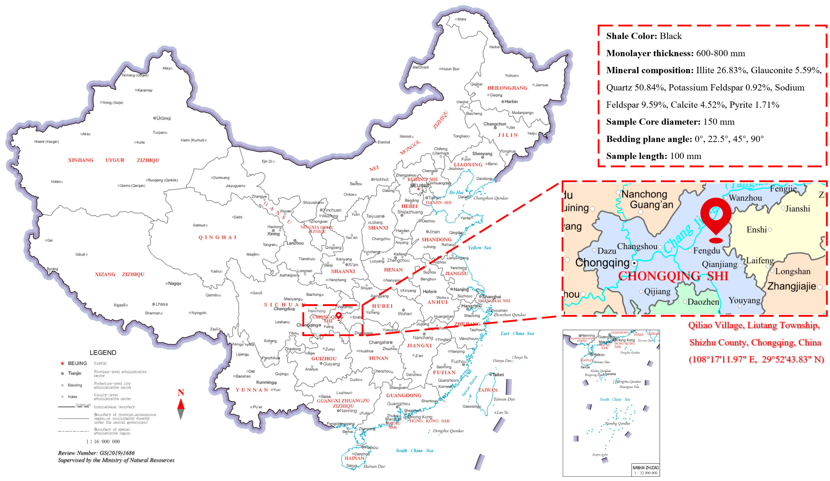
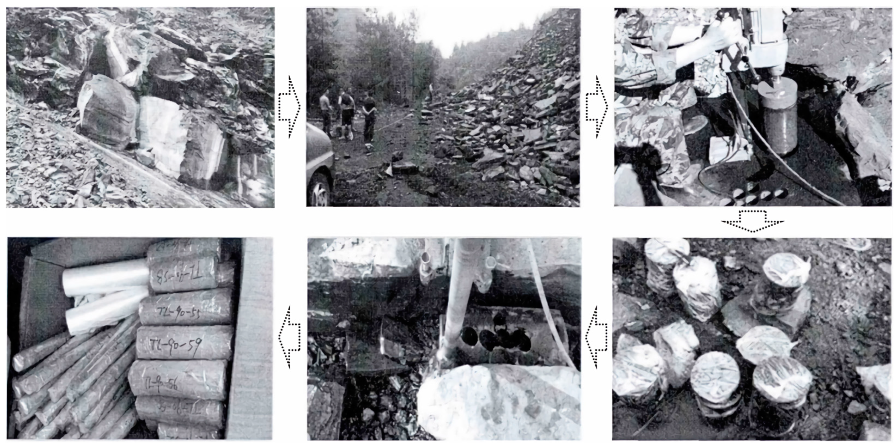
4.2. Eastern Yunnan–Western Chongqing Shale

4.2.1. Project Case

The bedding angle of shale significantly affects its mechanical behavior. To test the applicability of this model at different bedding angles, experimental data from Eastern Yunnan–Western Chongqing shale were used for validation. The Eastern Yunnan–Western Chongqing area is one of China’s key shale gas exploration and development regions, possessing abundant shale gas resources [107]. This region is rich in Silurian hydrocarbon source rocks, having undergone multiple phases of complex geological structural activities, and has long been in a state of uplift and erosion [108]. From a petrophysical evaluation perspective, the Silurian shales in the Eastern Yunnan–Western Chongqing area provide high-quality regional cap rocks for hydrocarbon reservoirs, characterized by strong continuity, large thickness, good sealing properties, high organic content, and well-developed maturity. The proven total natural gas resources reach 1.74 × 10¹² m³ [109]. The mechanical properties of shale are crucial for optimizing hydraulic fracturing techniques and addressing wellbore instability issues during extraction. Thus, Zhang [110] conducted a detailed investigation of the shale in this area. As shown in Figure 7, the sampling site is located in Qiliao Village, Liutang Township, Shizhu County, Chongqing (108°17′11.97″ E, 29°52′43.83″ N), a region geologically situated at the eastern margin of the Sichuan Basin, at the junction of the Sichuan Basin steep structural belt and the Eastern Yunnan–Western Chongqing transitional structural belt, belonging to the Lower Silurian Longmaxi Formation.

As shown in Figure 8, to ensure that the rock samples retain their original physical and mechanical properties during collection, samples were directly drilled from the rock using mechanical methods, or first, a cylindrical core with a diameter of 150 mm was drilled and then samples at different dip angles were extracted from it. Samples at angles of 0°, 22.5°, 45°, and 90° to the bedding planes were taken. After sampling, the samples needed to be quickly dried, labeled, wrapped in cling film, then wrapped with kraft paper, isolated with plastic, wax-sealed with numbers, and finally, boxed and transported to the laboratory. Subsequently, Zhang [110] conducted indoor microstructural analysis and triaxial compression tests on these samples, systematically studying the microstructure, elastic modulus, and compressive strength of the Eastern Yunnan–Western Chongqing shale.

4.2.2. Parameter Selection

Based on the physical and mechanical data of Eastern Yunnan–Western Chongqing shale provided by Zhang [110], further analysis was conducted on the applicability of the constitutive model under different bedding plane angles. As shown in Figure 9, to ensure the accuracy of the analysis, the calculation of the constitutive model adopted the same bedding plane angles as the indoor experiments, specifically including 0°, 22.5°, 45°, and 90°.

Based on indoor experimental data, a fitting analysis was conducted on the relationship between the compressive strength of shale and the angle of the bedding planes. Figure 10 displays the variation in compressive strength of shale under a confining pressure of 0 MPa.

The function f(θ) is used to predict changes in the stress–strain curves of shale at different bedding angles. The fitting curve passes exactly through the data points from the indoor experiment, demonstrating high fitting accuracy. Based on the fitting curve, the expression for function f(θ) is:

$$f(\theta )=2.2857{\sin }^3\theta -0.273{\sin }^2\theta -2.0498\sin \theta +1$$

(72)

Specific parameters are shown in

Table 2. Mechanical parameters of the elastoplastic damage coupled model for Eastern Yunnan–Western Chongqing shale [110].

Name	Value
Elastic parameters	E = 28.0 GPa, ν = 0.14
Plastic parameters	α1 = 0.8, α2 = 0.3, $\kappa$ = 87.5 MPa, h1 = 1.0, h0 = 3.6, b = 500
Damage parameters	ωc = 0.7, Bω = 0.5 MPa−1, r = 0.2
Damage softening parameters	a = 3.45exp(−0.047σ3) + 1

, where the physical and mechanical significance of each parameter is consistent with Table 1.

4.2.3. Verification Result

The mechanical parameters from Table 2 were input into the constitutive model to simulate and compare with the triaxial compression test data of Eastern Yunnan–Western Chongqing shale. Figure 11 shows the stress–strain curves at bedding plane angles of 0°, 22.5°, 45°, and 90° under different confining pressures. Here, the scatter points represent experimental data, and the solid lines are the computational results of the constitutive model. Comparing the theoretical curves with the experimental data, it is observable that the constitutive model effectively describes the increase in shale strength under high confining pressure, the nonlinear stage before peak strength, and the material softening caused by the evolution of internal microcracks after the yield point. As the confining pressure increases, the transverse strain of the rock body is inhibited, reducing the brittle behavior of the shale and enhancing its plastic behavior, thereby increasing peak strength. Figure 11b–d display the triaxial compression curves at bedding plane angles of 22.5°, 45°, and 90°, respectively, with stress–strain curve trends similar to Figure 11a. Notably, at a bedding plane angle of 45°, the strength of the shale is the lowest, and the theoretical curve aligns well with the indoor experimental data. Overall, the elastoplastic damage coupled constitutive model established in this paper accurately reflects the mechanical characteristics of shale under different confining pressures and bedding angles.

5. Model Parameter Sensitivity Analysis

In the constitutive model, the plastic hardening rate b, the damage evolution rate B_ω, the weighting coefficient r, and the damage softening a are four important coupled parameters requiring further parameter sensitivity analysis.

From Figure 12, during the pre-peak stage, b controls the rate of plastic hardening. A larger b value makes plastic hardening more pronounced and increases the peak strength. A smaller b enhances the nonlinear deformation. However, b has a minor impact on residual strength and damage evolution.

From Figure 13, it is evident that the damage evolution rate B_ω plays a role in elastoplastic and damage behavior. The value of B_ω has a minor impact on pre-peak deformation but a significant impact on post-peak deformation. The smaller B_ω is, the faster the post-peak stress decreases, the deformation under the same stress condition significantly increases, the post-peak residual stress notably reduces, and the rate of damage increase accelerates. A larger B_ω value implies a rapid development of the damage variable, enhancing the damage softening effect, accelerating the post-peak stress decrease, and leading to a reduction in peak strength.

From Figure 14, it is known that in the post-peak phase, the weighting coefficient r has a significant impact on plastic behavior and damage behavior. The larger r is, the slower the damage grows, and the smaller the stress peak and residual strength are. Where r = 0 indicates that only Y^P drives damage development, with no damage occurring during the elastic deformation phase, i.e., ω = 0. r = 0.5 means that Y^e and Y^P contribute equally to damage development.

From Figure 15, a reflects the degree of post-peak stress decrease. The larger a is, the faster the damage grows, the quicker the stress decreases, and the lower the peak and residual strengths are.

6. Conclusions

This paper combines plastic increment theory and irreversible thermodynamics to construct an elastoplastic damage coupled constitutive equation of layered rock, implemented numerically through the UMAT development in ABAQUS. The code for the elastoplastic damage coupled model has also been provided. By comparing indoor experimental data from La Biche shale in Canada and Eastern Yunnan–Western Chongqing shale in China, the model’s validity is verified, and the impact of model parameters on elastoplastic and damage behavior is analyzed. The main conclusions are as follows:

(1)

According to irreversible thermodynamics, the damage evolution equation is defined as a function related to damage and damage-driving force. Plastic body strain increments and equivalent plastic strain increments are used to build the plastic thermodynamic potential. Additionally, the effects of confining pressure and layered structure on shale mechanical behavior are considered. Furthermore, damage, plasticity, and elastoplastic damage are coupled corrected using the regression mapping algorithm and integrated into ABAQUS 2022 through the UMAT subroutine development.

(2)

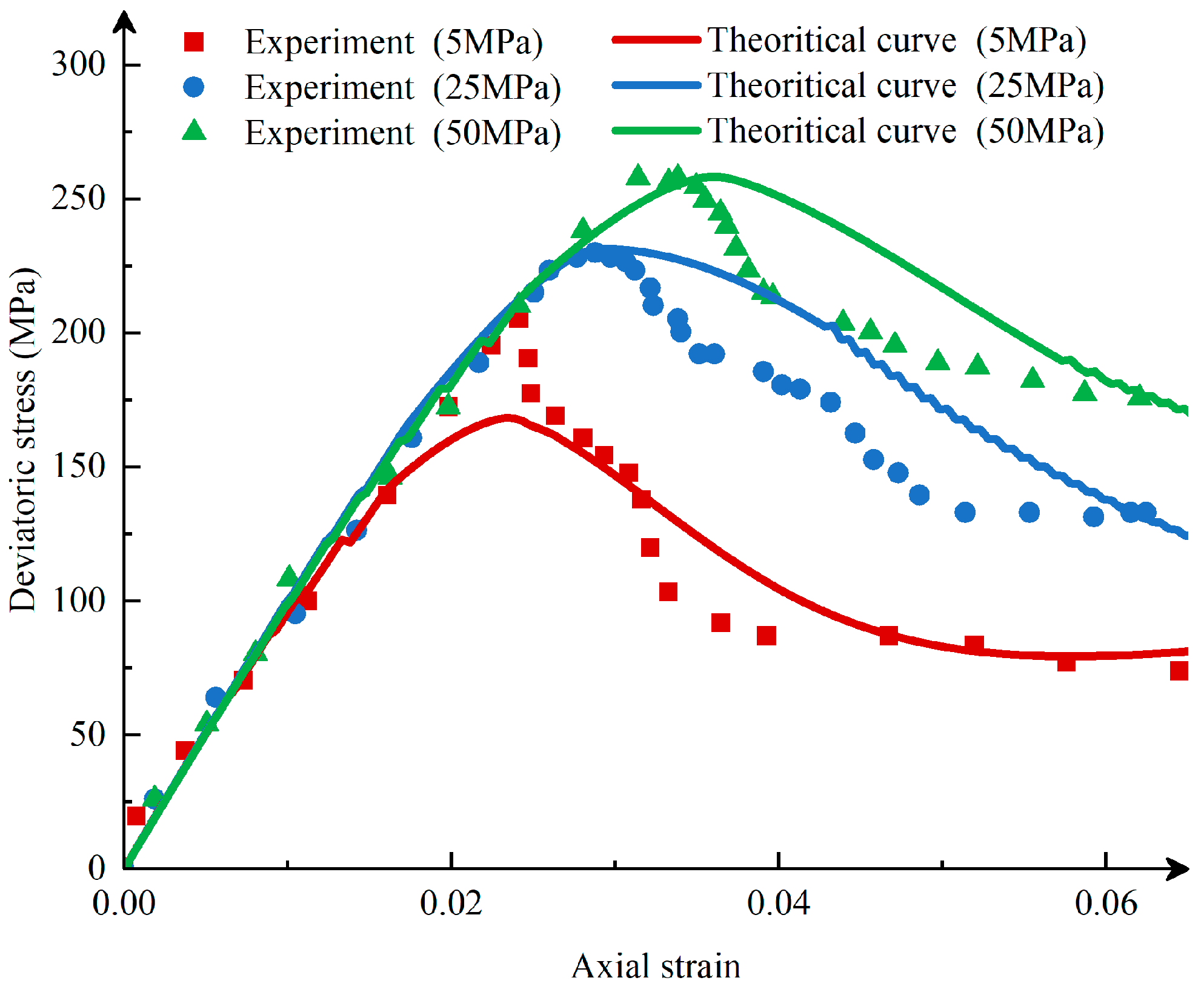
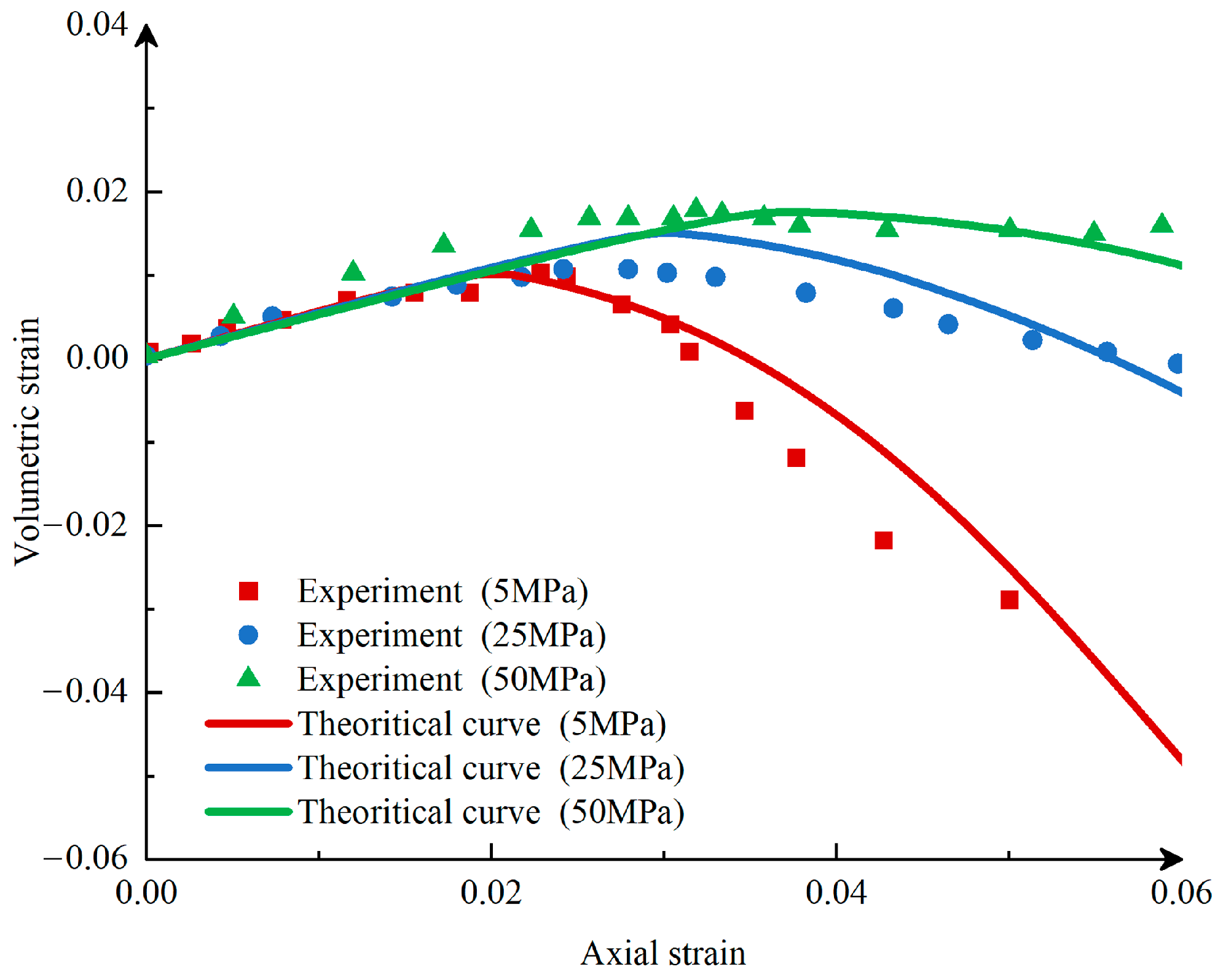
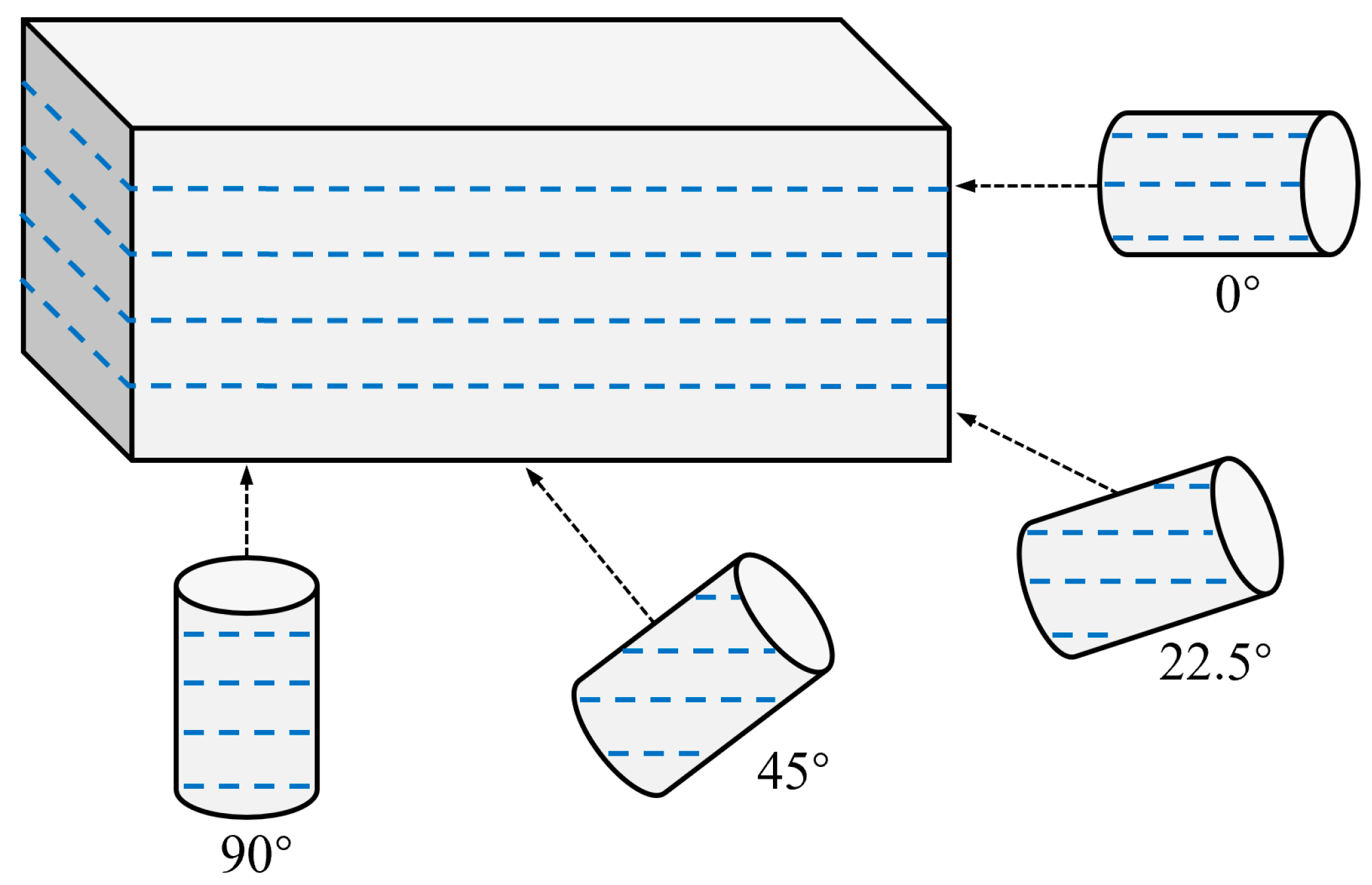
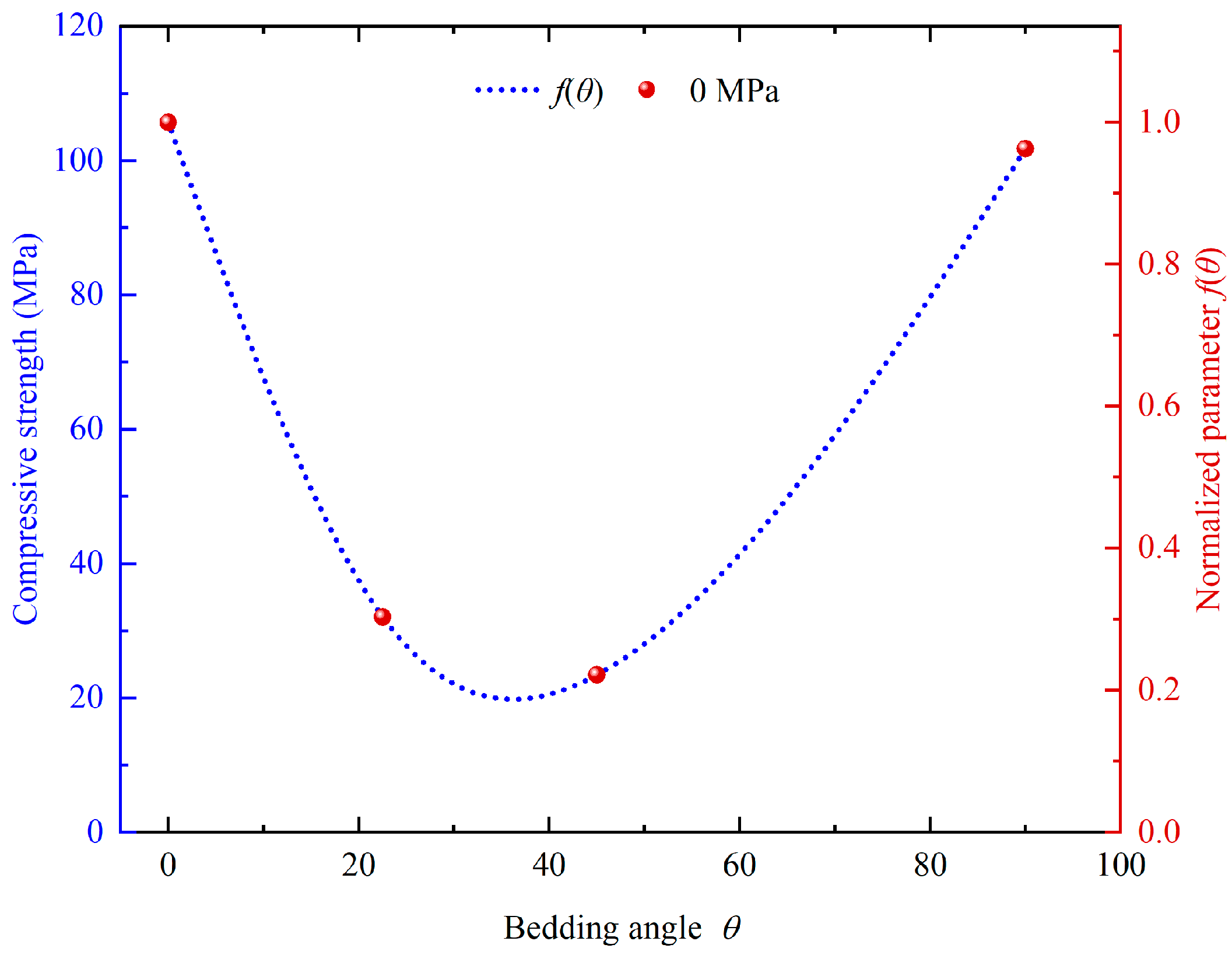
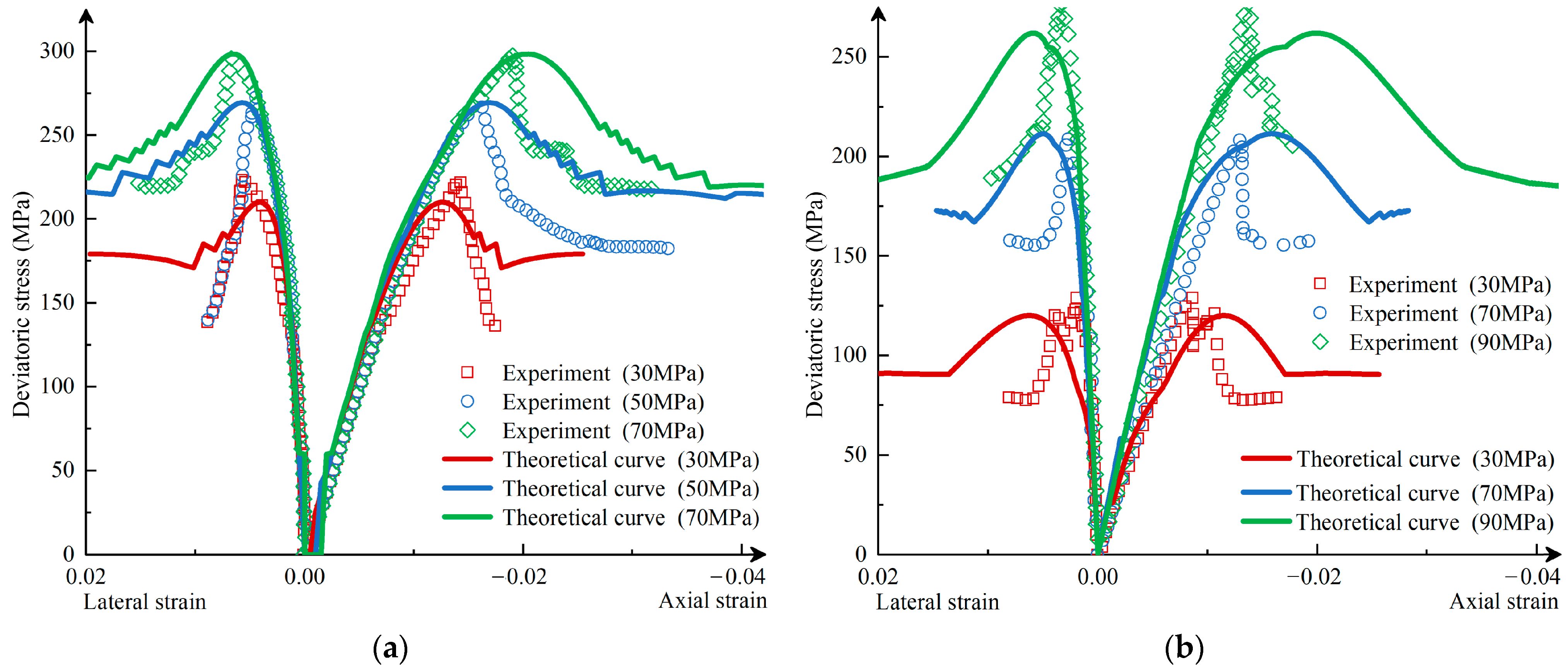
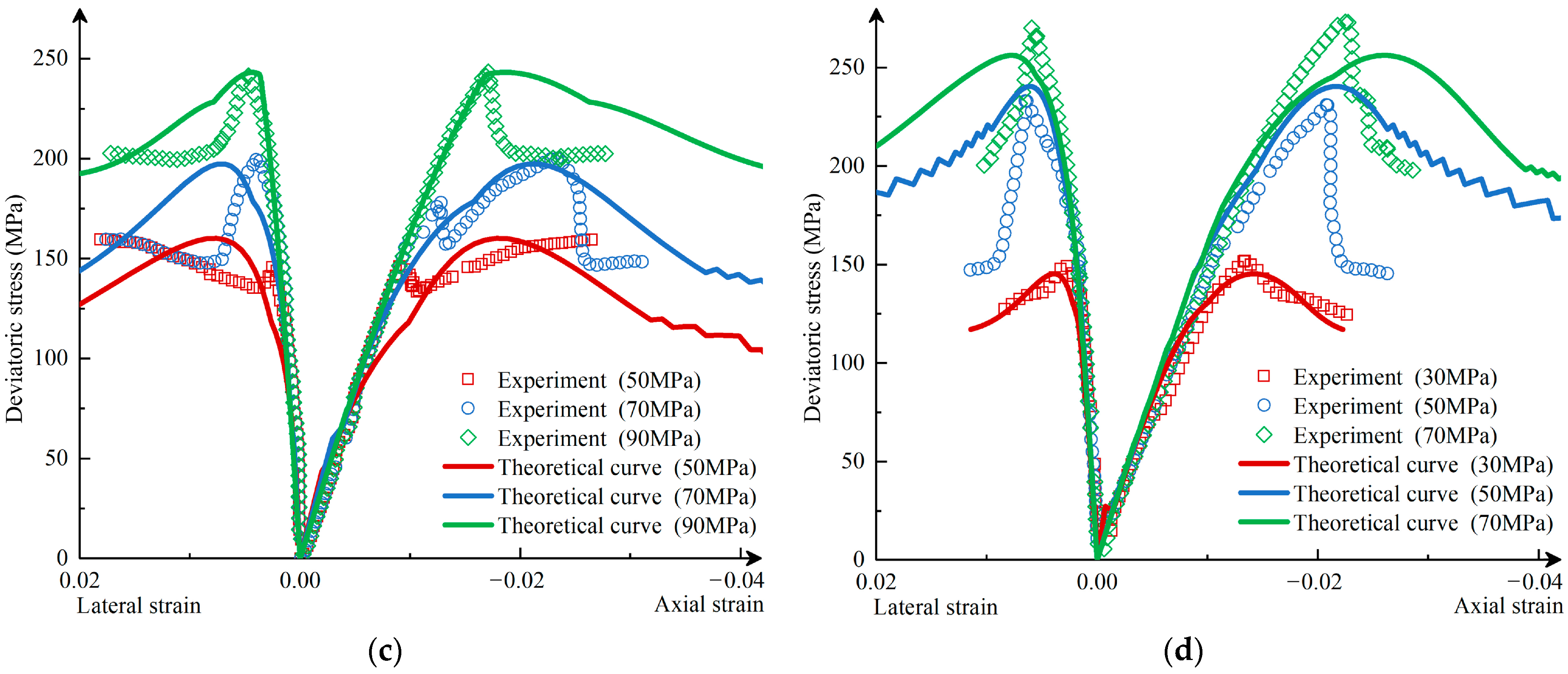
Simulation analysis of La Biche shale’s triaxial experiments shows that the model can reflect the characteristics of increased peak stress with confining pressure and decreased post-peak stress and simulate the volumetric expansion of shale under stress and the reduction in volumetric expansion with increased confining pressure. Further simulation analysis of the experimental data from Eastern Yunnan–Western Chongqing shale demonstrates that the constitutive model can effectively describe the increase in shale strength under high confining pressure, the macroscopic mechanical characteristics under different bedding plane angles, and the material softening behavior caused by the evolution of internal microcracks after the yield point.

(3)

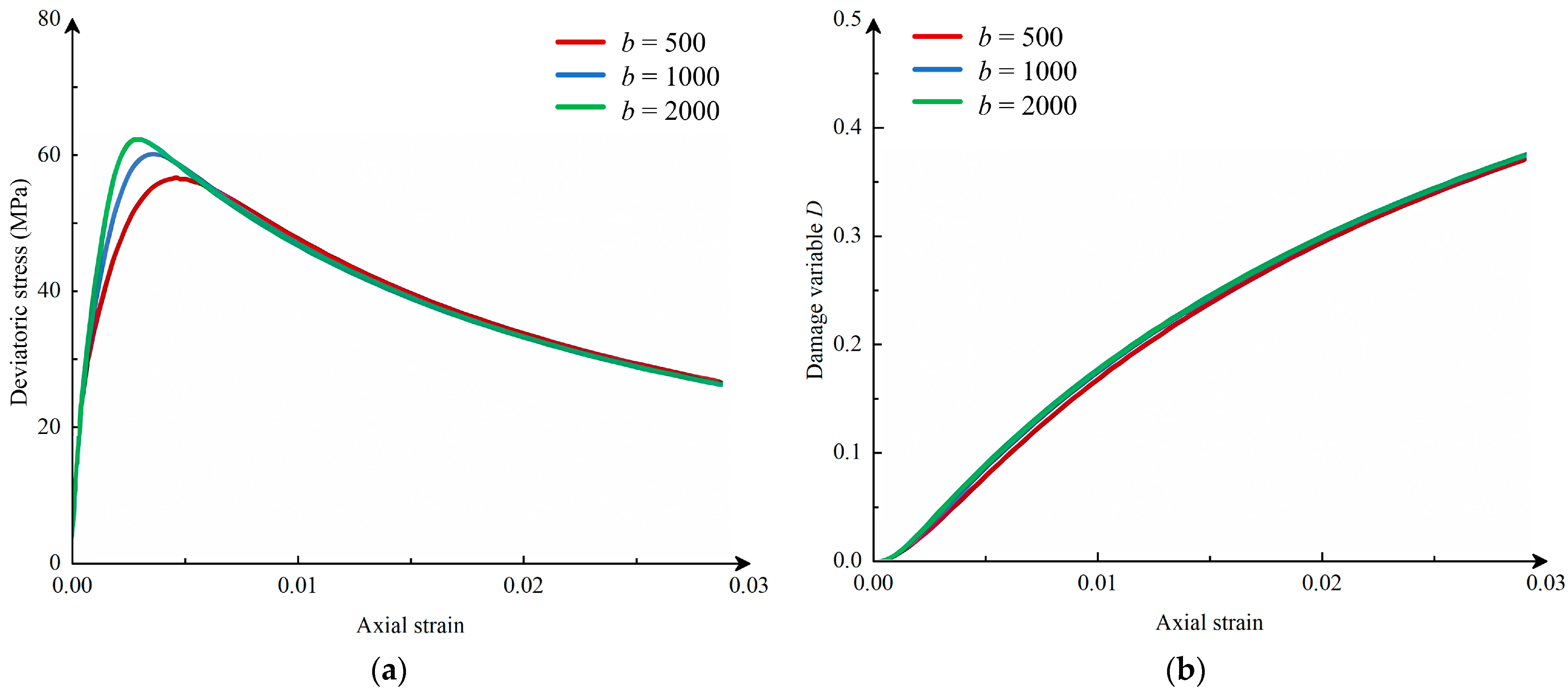
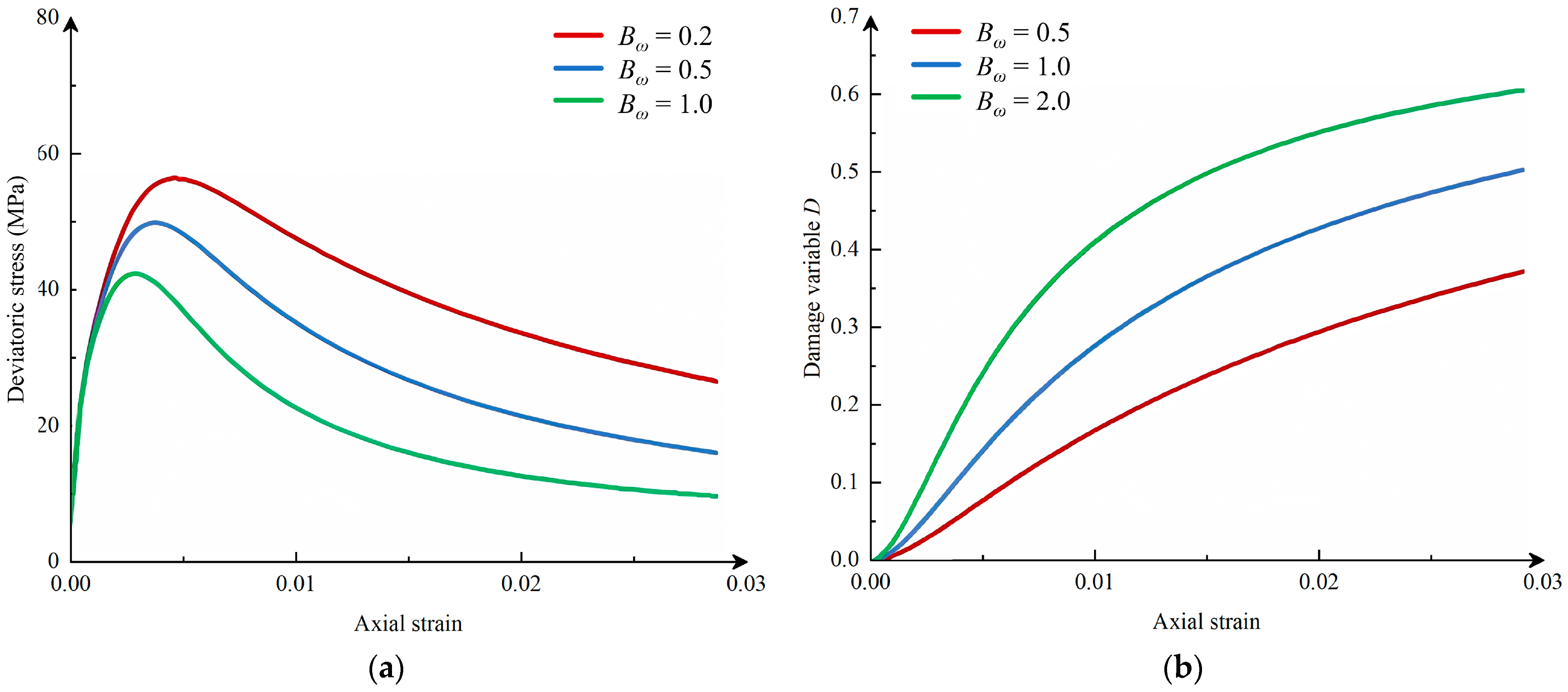
Through parameter sensitivity analysis, it is found that the plastic hardening rate b determines the plastic hardening. The larger b is, the more evident the plastic hardening and the greater the peak strength. The damage evolution rate B_ω affects the post-peak strain. The smaller B_ω is, the faster the post-peak stress decreases, and the greater the strain under the same stress condition. The weighting coefficient r reflects damage behavior. The larger r is, the slower the damage grows, and the smaller the stress peak and residual strength are. The damage softening a indicates the degree of post-peak stress decrease. The larger a is, the faster the stress decreases, and the lower the peak strength and residual strength are.

References

1. Laloui, L.; Ferrari, A. Multiphysical Testing of Soils and Shales; Heidelberg Press: Berlin, Germany, 2012; Available online: https://link.springer.com/book/10.1007/978-3-642-32492-5 (accessed on 3 October 2024).
2. Sie, C.Y.; Nguyen, Q.P. Field gas huff-n-puff for enhancing oil recovery in Eagle Ford shales—Effect of reservoir rock and crude properties. Fuel 2022, 328, 125127. [Google Scholar] [CrossRef]
3. Xia, L.Y.; Zhao, X.Y.; Wu, Y. Status, disadvantages, and prospects of oil shale in China: An economic perspective. Energy Policy 2023, 183, 113795. [Google Scholar] [CrossRef]
4. U.S. Geological Survey (USGS). World Petroleum Assessment. 1 January 2024. Available online: https://www.usgs.gov/centers/central-energy-resources-science-center/science/world-oil-and-gas-resource-assessments (accessed on 3 October 2024).
5. U.S. Energy Information Administration (EIA). Technically Recoverable Shale Oil and Shale Gas Resources: An Assessment of 137 Shale Formations in 41 Countries Outside the United States. 17 May 2013. Available online: https://www.eia.gov/analysis/studies/worldshalegas/pdf/overview.pdf (accessed on 3 October 2024).
6. International Energy Agency (IEA). World Energy Outlook 2023. 24 October 2023. Available online: https://www.iea.org/reports/world-energy-outlook-2023?wpappninja_v=b64a7tp1d (accessed on 3 October 2024).
7. Tong, X.G.; Zhang, G.Y.; Wang, Z.M.; Wen, Z.X.; Tian, Z.J.; Wang, H.J.; Ma, F.; Wu, Y.P. Distribution and potential of global oil and gas resources. Pet. Explor. Dev. 2018, 45, 779–789. [Google Scholar] [CrossRef]
8. British Petroleum (BP). bp Energy Outlook. 10 July 2024. Available online: https://www.bp.com/content/dam/bp/business-sites/en/global/corporate/pdfs/energy-economics/energy-outlook/bp-energy-outlook-2024.pdf (accessed on 3 October 2024).
9. British Petroleum (BP). Statistical Review of World Energy. 8 July 2021. Available online: https://www.bp.com/content/dam/bp/business-sites/en/global/corporate/pdfs/energy-economics/statistical-review/bp-stats-review-2021-full-report.pdf (accessed on 3 October 2024).
10. Economics & Technology Research Institute (ETRI). Oil and Gas Industry: 2023 Review and 2024 Outlook. 8 March 2024. Available online: https://www.cnpc.com.cn/en/nr2024/202403/66acc9d48164489392b0aa3e009f116b.shtml (accessed on 3 October 2024).
11. Qi, X.Y.; Geng, D.D.; Feng, M.Y.; Xu, M.Z. Study on failure characteristics and evaluation index of aquifer shale based on energy evolution. Acta Geotech. 2024, 1, 6691–6710. [Google Scholar] [CrossRef]
12. King, G.E. Hydraulic fracturing 101: What every representative, environmentalist, regulator, reporter, investor, university researcher, neighbor, and engineer should know about estimating frac risk and improving frac performance in unconventional gas and oil wells. In Proceedings of the SPE Hydraulic Fracturing Technology Conference, Woodlands, TX, USA, 6–8 February 2012. [Google Scholar] [CrossRef]
13. Jin, C.R.; Cusatis, G.L. New Frontiers in Oil and Gas Exploration; International Press: New York, NY, USA, 2016; Available online: https://link.springer.com/book/10.1007/978-3-319-40124-9 (accessed on 3 October 2024).
14. Li, W.P.; Zhang, D.M.; Li, M.H. Failure criteria of gas-infiltrated sandy shale based on the effective stress principle. Energies 2016, 9, 972. [Google Scholar] [CrossRef]
15. Li, W.; Liu, J.S.; Zeng, J.; Leong, Y.K.; Elsworth, D.; Tian, J.W.; Li, L. A fully coupled multidomain and multiphysics model for evaluation of shale gas extraction. Fuel 2020, 278, 118214. [Google Scholar] [CrossRef]
16. Heng, S.; Li, X.Z.; Liu, X.; Chen, Y. Experimental study on the mechanical properties of bedding planes in shale. J. Nat. Gas Sci. Eng. 2020, 76, 103161. [Google Scholar] [CrossRef]
17. Horii, H.; Nemat-Nasser, S. Compression-induced microcrack growth in brittle solids: Axial splitting and shear failure. J. Geophys. Res. Solid Earth 1985, 90, 3105–3125. [Google Scholar] [CrossRef]
18. Wong, R.C.K. Swelling and softening behaviour of La Biche shale. Can. Geotech. J. 1998, 35, 206–221. [Google Scholar] [CrossRef]
19. Li, C.B.; Bažant, Z.P.; Xie, H.P.; Rahimi-Aghdam, S. Anisotropic microplane constitutive model for coupling creep and damage in layered geomaterials such as gas or oil shale. Int. J. Rock Mech. Min. Sci. 2019, 124, 104074. [Google Scholar] [CrossRef]
20. Horsrud, P.; Sønstebø, E.F.; Bøe, R. Mechanical and petrophysical properties of North Sea shales. Int. J. Rock Mech. Min. Sci. 1998, 35, 1009–1020. [Google Scholar] [CrossRef]
21. Wang, J.L.; Liu, M.M.; Bentley, Y.M.; Feng, L.Y.; Zhang, C.H. Water use for shale gas extraction in the Sichuan Basin, China. J. Environ. Manag. 2018, 226, 13–21. [Google Scholar] [CrossRef] [PubMed]
22. Fan, Z.D.; Xie, H.P.; Sun, X.; Zhang, R.; Li, C.B.; Zhang, Z.T.; Xie, J.; Wang, J.; Ren, L. Crack deflection in shale-like layered rocks under three-point bend loading. Eng. Fract. Mech. 2023, 289, 109464. [Google Scholar] [CrossRef]
23. Niandou, H.; Shao, J.F.; Henry, J.P.; Fourmaintraux, D. Laboratory investigation of the mechanical behaviour of Tournemire shale. Int. J. Rock Mech. Min. Sci. 1997, 34, 3–16. [Google Scholar] [CrossRef]
24. Jaeger, J.C.; Cook, N.G.W.; Zimmerman, R.W. Fundamentals of Rock Mechanics; Blackwell Press: London, UK, 2007; Available online: https://www.researchgate.net/publication/220010592 (accessed on 3 October 2024).
25. Mou, P.W.; Pan, J.N.; Wang, K.; Wei, J.; Yang, Y.H.; Wang, X.L. Influences of hydraulic fracturing on microfractures of high-rank coal under different in-situ stress conditions. Fuel 2021, 287, 119566. [Google Scholar] [CrossRef]
26. Zhou, H.; Zhang, K.; Feng, X. A Coupled Elasto-Plastic-Damage Mechanical Model for Marble. Sci. China Technol. Sci. 2011, 54, 228–234. [Google Scholar] [CrossRef]
27. Liu, W.B.; Zhang, S.G. An improved unsteady creep model based on the time dependent mechanical parameters. Mech. Adv. Mater. Struct. 2021, 28, 1838–1848. [Google Scholar] [CrossRef]
28. Qiu, S.L.; Feng, X.T.; Xiao, J.Q.; Zhang, C.Q. An experimental study on the pre-peak unloading damage evolution of marble. Rock Mech. Rock Eng. 2014, 47, 401–419. [Google Scholar] [CrossRef]
29. Cerfontaine, B.; Charlier, R.; Collin, F.; Taiebat, M. Validation of a new elastoplastic constitutive model dedicated to the cyclic behaviour of brittle rock materials. Rock Mech. Rock Eng. 2017, 50, 2677–2694. [Google Scholar] [CrossRef]
30. Meng, X.J.; Geng, D.; Liu, S.K. The modified Mohr-Coulomb model considering softening effect and intermediate principal stress. Mech. Adv. Mater. Struct. 2024, 1–15. [Google Scholar] [CrossRef]
31. Li, Q.; Franci, A.; Li, H.; Li, P.; Li, T.L.; Shang, C.S. Modified discontinuous deformation analysis with mixed bilinear failure model for investigating quasi-brittle failure in geo-materials. Comput. Geotech. 2024, 173, 106536. [Google Scholar] [CrossRef]
32. Shao, J.F.; Zhu, Q.Z.; Su, K. Modeling of creep in rock materials in terms of material degradation. Comput. Geotech. 2003, 30, 549–555. [Google Scholar] [CrossRef]
33. He, J.L.; Niu, F.J.; Su, W.J.; Jiang, H.Q. Nonlinear unified strength criterion for frozen soil based on homogenization theory. Mech. Adv. Mater. Struct. 2023, 30, 4002–4015. [Google Scholar] [CrossRef]
34. Zhu, Q.Z.; Kondo, D.; Shao, J.F. Micromechanical analysis of coupling between anisotropic damage and friction in quasi-brittle materials: Role of the homogenization scheme. Int. J. Solids Struct. 2008, 45, 1385–1405. [Google Scholar] [CrossRef]
35. Zhu, Q.Z.; Zhou, C.B.; Shao, J.F.; Kondo, D. A discrete thermodynamic approach for anisotropic plastic-damage modeling of cohesive-frictional geomaterials. Int. J. Numer. Anal. Methods Geomech. 2010, 34, 1250–1270. [Google Scholar] [CrossRef]
36. Unteregger, D.; Fuchs, B.; Hofstetter, G. A damage plasticity model for different types of intact rock. Int. J. Rock Mech. Min. Sci. 2015, 80, 402–411. [Google Scholar] [CrossRef]
37. Wang, H.Y.; Zhang, Q.; Wu, P.N.; Li, Y.J.; Han, L.J.; Han, G.L. Elastoplastic solution of a circular tunnel in surrounding rock with any nonlinear yield criteria and plastic flow envelopes. Comput. Geotech. 2024, 166, 105954. [Google Scholar] [CrossRef]
38. Kamdem, T.C.; Richard, K.G.; Béda, T. Modeling the mechanical behavior of rock during plastic flow using fractional calculus theory. Appl. Math. Model. 2024, 130, 790–805. [Google Scholar] [CrossRef]
39. Sarout, J.; Molez, L.; Guéguen, Y.; Hoteit, N. Shale dynamic properties and anisotropy under triaxial loading: Experimental and theoretical investigations. Phys. Chem. Earth 2007, 32, 896–906. [Google Scholar] [CrossRef]
40. Zhu, Q.Z.; Shao, J.F.; Mainguy, M. A micromechanics-based elastoplastic damage model for granular materials at low confining pressure. Int. J. Plast. 2010, 26, 586–602. [Google Scholar] [CrossRef]
41. Li, Y.K.; Du, B.; Shen, M.X. A nonlinear creep model for transversely isotropic rock based on fractional calculus theory. Mech. Adv. Mater. Struct. 2023, 1–11. [Google Scholar] [CrossRef]
42. Sone, H.; Zoback, M.D. Mechanical properties of shale-gas reservoir rocks—Part 1: Static and dynamic elastic properties and anisotropy. Geophysics 2013, 78, 381–392. [Google Scholar] [CrossRef]
43. Sone, H.; Zoback, M.D. Time-dependent deformation of shale gas reservoir rocks and its long-term effect on the in situ state of stress. Int. J. Rock Mech. Min. Sci. 2014, 69, 120–132. [Google Scholar] [CrossRef]
44. Mousavi Nezhad, M.; Fisher, Q.J.; Gironacci, E.; Rezania, M. Experimental study and numerical modeling of fracture propagation in shale rocks during Brazilian disk test. Rock Mech. Rock Eng. 2018, 51, 1755–1775. [Google Scholar] [CrossRef]
45. Ip, S.C.; Choo, J.; Borja, R.I. Impacts of saturation-dependent anisotropy on the shrinkage behavior of clay rocks. Acta Geotech. 2021, 16, 3381–3400. [Google Scholar] [CrossRef]
46. Ip, S.C.; Borja, R.I. Multiscale interactions of elastic anisotropy in unsaturated clayey rocks using a homogenization model. Acta Geotech. 2023, 18, 2289–2307. [Google Scholar] [CrossRef]
47. Ip, S.C.; Borja, R.I. Evolution of anisotropy with saturation and its implications for the elastoplastic responses of clay rocks. Int. J. Numer. Anal. Methods Geomech. 2022, 46, 23–46. [Google Scholar] [CrossRef]
48. Cao, Y.J.; Wang, W.; Shen, W.Q.; Cui, X.Y.; Shao, J.F. A new hybrid phase-field model for modeling mixed-mode cracking process in anisotropic plastic rock-like materials. Int. J. Plast. 2022, 157, 103395. [Google Scholar] [CrossRef]
49. Dragon, A.; Mroz, Z. A continuum model for plastic-brittle behaviour of rock and concrete. Internat. J. Engrg. Sci. 1979, 17, 121–137. [Google Scholar] [CrossRef]
50. Frantziskonis, G.; Desai, C. Elastoplastic model with damage for strain softening geomaterials. Acta Mech. 1987, 68, 151–170. [Google Scholar] [CrossRef]
51. Rouabhi, A.; Tijani, M.; Rejeb, A. Triaxial behaviour of transversely isotropic materials: Application to sedimentary rocks. Int. J. Numer. Anal. Methods Geomech. 2007, 31, 1517–1535. [Google Scholar] [CrossRef]
52. Chen, L.; Wang, C.P.; Liu, J.F.; Liu, J.; Wang, J.; Jia, Y.; Shao, J.F. Damage and plastic deformation modeling of Beishan granite under compressive stress conditions. Rock Mech. Rock Eng. 2015, 48, 1623–1633. [Google Scholar] [CrossRef]
53. Zhang, J.C.; Xu, W.Y.; Wang, H.L.; Wang, R.B.; Meng, Q.X. Testing and modeling of the mechanical behavior of dolomite in the Wudongde hydropower plant. Geomech. Geoeng. 2016, 11, 270–280. [Google Scholar] [CrossRef]
54. Zhao, Y.; Semnani, S.J.; Yin, Q.; Borja, R.I. On the strength of transversely isotropic rocks. Int. J. Numer. Anal. Methods Geomech. 2018, 42, 1917–1934. [Google Scholar] [CrossRef]
55. Kraipru, K.; Fuenkajorn, K.; Thongprapha, T. The effect of transverse isotropy on the creep behavior of bedded salt under confining pressures. Mech. Time-Depend. Mater. 2024, 28, 2879–2897. [Google Scholar] [CrossRef]
56. Duan, S.Q.; Liu, S.H.; Xiong, J.C.; Xu, D.P.; Xu, L.B.; Jiang, X.Q.; Zhang, M.H.; Liu, G.F. Investigation on uncoordinated deformation and failure mechanism and damage modeling of rock mass with weak interlayer zone. Eng. Fail. Anal. 2024, 163, 108563. [Google Scholar] [CrossRef]
57. Cauvin, A.; Testa, R.B. Damage mechanics: Basic variables in continuum theories. Int. J. Solids Struct. 1999, 36, 747–761. [Google Scholar] [CrossRef]
58. Challamel, N.; Lanos, C.; Casandjian, C. Strain-based anisotropic damage modelling and unilateral effects. Int. J. Mech. Sci. 2005, 47, 459–473. [Google Scholar] [CrossRef]
59. Liu, S.J.; Wang, Z.Q.; Kou, M.M.; Zhang, Y.J.; Wang, Y.L. Phase-field simulations of unloading failure behaviors in rock and rock-like materials. Theor. Appl. Fract. Mech. 2023, 126, 103936. [Google Scholar] [CrossRef]
60. Lu, J.F.; Yin, T.B.; Guo, W.X.; Men, J.Q.; Ma, J.X.; Yang, Z.; Chen, D.C. Dynamic response and constitutive model of damaged sandstone after triaxial impact. Eng. Fail. Anal. 2024, 163, 108450. [Google Scholar] [CrossRef]
61. Zhang, J.C. Experimental and modelling investigations of the coupled elastoplastic damage of a quasi-brittle rock. Rock Mech. Rock Eng. 2018, 51, 465–478. [Google Scholar] [CrossRef]
62. Li, Y.Q.; Huang, D.; Song, Y. Energy evolution and damage model of sandstone under seepage-creep-disturbance loading. Mech. Adv. Mater. Struct. 2024, 1–21. [Google Scholar] [CrossRef]
63. Pensée, V.; Kondo, D.; Dormieux, L. Micromechanical analysis of anisotropic damage in brittle materials. J. Eng. Mech. 2002, 128, 889–897. [Google Scholar] [CrossRef]
64. Hu, D.W.; Zhu, Q.Z.; Zhou, H.; Shao, J.F. A discrete approach for anisotropic plasticity and damage in semi-brittle rocks. Comput. Geotech. 2010, 37, 658–666. [Google Scholar] [CrossRef]
65. Xie, N.; Zhu, Q.Z.; Xu, L.H.; Shao, J.F. A micromechanics-based elastoplastic damage model for quasi-brittle rocks. Comput. Geotech. 2011, 38, 970–977. [Google Scholar] [CrossRef]
66. Zhu, Q.Z.; Shao, J.F. A refined micromechanical damage-friction model with strength prediction for rock-like materials under compression. Int. J. Solids Struct. 2015, 60–61, 75–83. [Google Scholar] [CrossRef]
67. Shao, J.F.; Jia, Y.; Kondo, D.; Chiarelli, A. A coupled elastoplastic damage model for semi-brittle materials and extension to unsaturated conditions. Mech. Mater. 2006, 38, 218–232. [Google Scholar] [CrossRef]
68. Parisio, F.; Samat, S.; Laloui, L. Constitutive analysis of shale: A coupled damage plasticity approach. Int. J. Solids Struct. 2015, 75–76, 88–98. [Google Scholar] [CrossRef]
69. Zhang, J.C.; Xu, W.Y.; Wang, H.L.; Wang, R.B.; Meng, Q.X.; Du, S.W. A coupled elastoplastic damage model for brittle rocks and its application in modelling underground excavation. Int. J. Rock Mech. Min. Sci. 2016, 84, 130–141. [Google Scholar] [CrossRef]
70. Ma, S.Q.; Gutierrez, M.; Hou, Z.K. Coupled plasticity and damage constitutive model considering residual shear strength for shales. Int. J. Geomech. 2020, 20, 04020109. [Google Scholar] [CrossRef]
71. Chen, H.G.; Zhao, C.; Zhang, R.; Xing, J.Q.; Huang, L.; Qian, Y. Macro-micro damage model of the effect of freeze-thaw on jointed rocks considering compaction deformation. Eng. Fail. Anal. 2023, 151, 107407. [Google Scholar] [CrossRef]
72. Shao, J.F.; Chau, K.T.; Feng, X.T. Modeling of anisotropic damage and creep deformation in brittle rocks. Int. J. Rock Mech. Min. Sci. 2006, 43, 582–592. [Google Scholar] [CrossRef]
73. Leoni, M.; Karstunen, M.; Vermeer, P. Anisotropic creep model for soft soils. Geotechnique 2008, 58, 215–226. [Google Scholar] [CrossRef]
74. Liu, X.S.; Ning, J.G.; Tan, Y.L.; Gu, Q.H. Damage constitutive model based on energy dissipation for intact rock subjected to cyclic loading. Int. J. Rock Mech. Min. Sci. 2016, 85, 27–32. [Google Scholar] [CrossRef]
75. Song, Z.Y.; Konietzky, H.; Frühwirt, T. Hysteresis energy-based failure indicators for concrete and brittle rocks under the condition of fatigue loading. Int. J. Fatigue 2018, 114, 298–310. [Google Scholar] [CrossRef]
76. Wang, X.L.; Zhao, Y.X.; Gao, Y.R.; Sun, Z.; Liu, B.; Jiang, Y.D. Energy evolution of anthracite considering anisotropy under high confining pressure: An experimental investigation. J. Rock Mech. Rock Eng. 2023, 56, 6735–6759. [Google Scholar] [CrossRef]
77. Rummel, F.; Fairhurst, C. Determination of the post-failure behavior of brittle rock using a servo-controlled testing machine. Rock Mech. 1970, 2, 189–204. [Google Scholar] [CrossRef]
78. Murakami, S.; Kamiya, K. Constitutive and damage evolution equations of elastic-brittle materials based on irreversible thermodynamics. Int. J. Mech. Sci. 1997, 39, 473–486. [Google Scholar] [CrossRef]
79. Peng, Y.Y.; Zhou, C.; Fu, C.F.; Zhong, Z.; Wang, J.J. Study on energy damage evolution of multi-flaw sandstone with different flaw lengths. Theor. Appl. Fract. Mech. 2024, 132, 104469. [Google Scholar] [CrossRef]
80. Zhai, Y.; Meng, F.D.; Li, Y.B.; Li, Y.; Zhao, R.F.; Zhang, Y.S. Research on dynamic compression failure characteristics and damage constitutive model of sandstone after freeze-thaw cycles. Eng. Fail. Anal. 2022, 140, 106577. [Google Scholar] [CrossRef]
81. Lemaitre, J. Evaluation of dissipation and damage in metals submitted to dynamic loading. Int. Conf. Mech. Behav. Mater. 1971, 5, 329–345. [Google Scholar] [CrossRef]
82. Salari, M.R.; Saeb, S.A.; Willam, K.J.; Patchet, S.J.; Carrasco, R.C. A coupled elastoplastic damage model for geomaterials. Comput. Methods Appl. Mech. Eng. 2004, 193, 2625–2643. [Google Scholar] [CrossRef]
83. Yang, S.Q.; Jing, H.W.; Wang, S.Y. Experimental investigation on the strength, deformability, failure behavior and acoustic emission locations of red sandstone under triaxial compression. Rock Mech. Rock Eng. 2012, 45, 583–606. [Google Scholar] [CrossRef]
84. Zhao, X.G.; Cai, M.; Wang, J.; Ma, L.K. Damage stress and acoustic emission characteristics of the Beishan granite. Int. J. Rock Mech. Min. Sci. 2013, 64, 258–269. [Google Scholar] [CrossRef]
85. Lubarda, V. On thermodynamic potentials in linear thermoelasticity. Int. J. Solids Struct. 2004, 41, 7377–7398. [Google Scholar] [CrossRef]
86. Kolomiets, V.I.; Bekker, A.T. Level of allowable stresses under cyclic variable-polarity thermal fields impact to concretes. In Proceedings of the ISOPE Pacific/Asia Offshore Mechanics Symposium, Vladivostok, Russia, 12–16 September 2004; Available online: https://onepetro.org/ISOPEPACOMS/proceedings-abstract/PACOMS04/All-PACOMS04/25687 (accessed on 3 October 2024).
87. Drucker, D.C.; Prager, W. Soil mechanics and plastic analysis or limit design. Q. Appl. Math. 1952, 10, 157–165. [Google Scholar] [CrossRef]
88. Ding, X.; Chen, N.; Zhang, F.; Zhang, G.Q. Evolution of strength parameters for sandstone specimens during triaxial compression tests. Adv. Civ. Eng. 2021, 2021, 8856743. [Google Scholar] [CrossRef]
89. Bennett, K.C.; Regueiro, R.A.; Luscher, D.J. Anisotropic finite hyper-elastoplasticity of geomaterials with Drucker-Prager/cap type constitutive model formulation. Int. J. Plast. 2019, 123, 224–250. [Google Scholar] [CrossRef]
90. Chen, P.J.; Dai, X.W.; Baldino, S.; Huang, T.; Deng, X.; Tan, Z.H.; Yan, S. A continuous surface cap model and computational framework for shale under high confining pressure. Geoenergy Sci. Eng. 2023, 230, 212186. [Google Scholar] [CrossRef]
91. Zhang, S.K.; Liao, S.Z.; Li, S.M.; Hu, J.H. Influence of engineering parameters on fracture vertical propagation in deep shale reservoir: A numerical study based on FEM. ACS Omega 2024, 9, 4635–4646. [Google Scholar] [CrossRef]
92. Saroglou, H.; Tsiambaos, G. A modified Hoek-Brown failure criterion for anisotropic intact rock. Int. J. Rock Mech. Min. Sci. 2008, 45, 223–234. [Google Scholar] [CrossRef]
93. Ismael, M.A.; Imam, H.F.; El-Shayeb, Y. A simplified approach to directly consider intact rock anisotropy in Hoek-Brown failure criterion. J. Rock Mech. Geotech. Eng. 2014, 6, 486–492. [Google Scholar] [CrossRef]
94. Zheng, Y.N.; Jia, C.J.; Zhang, S.; Shi, C. Experimental and constitutive modeling of the anisotropic mechanical properties of shale subjected to thermal treatment. Geomech. Energy Environ. 2023, 35, 100485. [Google Scholar] [CrossRef]
95. Winhausen, L.; Khaledi, K.; Jalali, M.; Bretthauer, M.; Amann, F. The anisotropic behavior of a clay shale: Strength, hydro-mechanical couplings, and failure processes. J. Geophys. Res. Solid Earth 2023, 128, e2023JB027382. [Google Scholar] [CrossRef]
96. Jia, C.J.; Zhang, S.; Xu, W.Y. Experimental investigation and numerical modeling of coupled elastoplastic damage and permeability of saturated hard rock. Rock Mech. Rock Eng. 2021, 54, 1151–1169. [Google Scholar] [CrossRef]
97. Krajcinovic, D.; Silva, M.A.G. Statistical aspects of the continuous damage theory. Int. J. Solids Struct. 1982, 18, 551–562. [Google Scholar] [CrossRef]
98. Cao, W.G.; Zhao, H.; Li, X.; Zhang, Y.J. Statistical damage model with strain softening and hardening for rocks under the influence of voids and volume changes. Can. Geotech. J. 2010, 47, 857–871. [Google Scholar] [CrossRef]
99. Zhao, H.; Shi, C.J.; Zhao, M.H.; Li, X.B. Statistical damage constitutive model for rocks considering residual strength. Int. J. Geomech. 2017, 17, 04016033. [Google Scholar] [CrossRef]
100. Clausen, J.; Damkilde, L.; Andersen, L. An efficient return algorithm for non-associated plasticity with linear yield criteria in principal stress space. Comput. Struct. 2007, 85, 1795–1807. [Google Scholar] [CrossRef]
101. Huang, J.; Griffiths, D.V. Observations on return mapping algorithms for piecewise linear yield criteria. Int. J. Geomech. 2008, 8, 253–265. [Google Scholar] [CrossRef]
102. Rahman, A.; Shahriar, M.S.; Timms, G.; Lindley, C.; Davie, A.B.; Biggins, D.; Hellicar, A.; Sennersten, C.; Smith, G.; Coombe, M. A machine learning approach to find association between imaging features and XRF signatures of rocks in underground mines. In Proceedings of the 2015 IEEE Sensors, Busan, Republic of Korea, 1–4 November 2015. [Google Scholar] [CrossRef]
103. Zhang, T.; Xu, W.Y.; Wang, H.L.; Wang, R.B.; Xu, J.R.; Hu, M.T. Experimental investigation on hydromechanical behavior of basalt and numerical modeling by return mapping algorithms. Bull. Eng. Geol. Environ. 2023, 82, 132. [Google Scholar] [CrossRef]
104. McCrossan, R.G.; Glaister, R.P.; Austin, G.H.; Nelson, S.J. Upper Cretaceous. In Geological History of Western Canada. Alta. Soc. Petr. Geol. 1970, 12, 169–188. [Google Scholar] [CrossRef]
105. Hein, F.J.; Cotterill, D.K. The Athabasca oil sands—A regional geological perspective, Fort McMurray area, Alberta, Canada. Nat. Resour. Res. 2006, 15, 85–102. [Google Scholar] [CrossRef]
106. Pinyol, N.; Vaunat, J.; Alonso, E.E. A constitutive model for soft clayey rocks that includes weathering effects. In Stiff Sedimentary Clays: Genesis and Engineering Behaviour: Géotechnique Symposium in Print 2007; ICE Publishing: London, UK, 2007; pp. 193–207. [Google Scholar] [CrossRef]
107. Huo, L.; Yang, C.H.; Mao, H.J.; Liu, J.X.; Yuan, Y.S. Experimental research on mechanical properties of western Hubei-Eastern Chongqing carbonaceous shale cap rock under unloading stress path. Chin. J. Rock Mech. Eng. 2016, 35 (Suppl. S1), 2898–2906. [Google Scholar] [CrossRef]
108. Yuan, Y.S.; Lin, J.H.; Cheng, X.Y.; Li, S.J. Yanshan—Himalayan denudation in Western Hubei—Eastern Chongqing. Chin. J. Geophys. 2014, 57, 2878–2884. [Google Scholar] [CrossRef]
109. Guo, Z.F.; Chen, M.K.; Fu, Y.X.; Chen, X.H. Natural gas reservoiring conditions of Sinian and Cambrian from western Hubei to eastern Chongqing areas. J. Southwest Pet. Univ. Sci. Technol. 2008, 30, 3–5. [Google Scholar] [CrossRef]
110. Zhang, Y.Z. Study on anisotropy of mechanical properties of the shale in West Hubei and East Chongqing. Master’s Thesis, Southwest University of Science and Technology, Mianyang City, China, 1 July 2016. Available online: https://cdmd.cnki.com.cn/Article/CDMD-10619-1016118914.htm (accessed on 3 October 2024).
Figure 1. Map of basins with assessed shale oil and shale gas formations [5].
Applsci 14 10923 g001
Figure 2. Loading direction and bedding plane angle θ.
Applsci 14 10923 g002
Figure 3. Principle of the regression mapping algorithm.
Applsci 14 10923 g003
Figure 4. Schematic of the calculation process for the elastoplastic damage coupled model.
Applsci 14 10923 g004
Figure 5. Stress–strain curves of theoretical and experimental for La Biche shale [18].
Applsci 14 10923 g005
Figure 6. Volumetric–axial strain curves of theoretical and experimental for La Biche shale [18].
Applsci 14 10923 g006
Figure 7. Location of Eastern Yunnan–Western Chongqing shale.
Applsci 14 10923 g007
Figure 8. Field sampling (modified from Zhang [110]).
Applsci 14 10923 g008
Figure 9. Samples in different bedding plane orientations.
Applsci 14 10923 g009
Figure 10. Fitting curve of f(θ) at 0 MPa confining pressure [110].
Applsci 14 10923 g010
Figure 11. Stress–strain curves of theoretical and experimental for Eastern Yunnan–Western Chongqing shale: (a) Comparison when the bedding angle θ is 0°; (b) Comparison when the bedding angle θ is 22.5°; (c) Comparison when the bedding angle θ is 45°; (d) Comparison when the bedding angle θ is 90° [110].
Applsci 14 10923 g011aApplsci 14 10923 g011b
Figure 12. Sensitivity analysis of b: (a) The relationship between axial strain and deviatoric stress; (b) The relationship between axial strain and damage variable D.
Applsci 14 10923 g012
Figure 13. Sensitivity analysis of Bω: (a) The relationship between axial strain and deviatoric stress; (b) The relationship between axial strain and damage variable D.
Applsci 14 10923 g013
Figure 14. Sensitivity analysis of r: (a) The relationship between axial strain and deviatoric stress; (b) The relationship between axial strain and damage variable D.
Applsci 14 10923 g014
Figure 15. Sensitivity analysis of a: (a) The relationship between axial strain and deviatoric stress; (b) The relationship between axial strain and damage variable D.
Applsci 14 10923 g015