Three-Dimensional Air Quality Monitoring and Simulation of Campus Microenvironment Based on UAV Platform

Abstract

This study innovatively employs drones equipped with air quality sensors to collect three-dimensional air quality data in a campus microenvironment. Data are accurately corrected using a BP neural network, and a cubic model is constructed using three-dimensional interpolation. Combining photogrammetry technology, this study analyzes air quality patterns, finding significant differences from macro trends. Construction activities and large electronic experimental equipment significantly increase PM_2.5 levels in the air. In rainy weather, the respiration of vegetation is enhanced, leading to higher CO₂ concentrations, while water bodies exhibit higher temperatures in rainy weather due to their high specific heat capacity. This research not only provides a new perspective for microenvironment air quality monitoring but also offers a scientific basis for future air quality monitoring and management.

1. Introduction

The concept of a geographical microenvironment pertains to local environmental conditions and characteristics within a relatively small spatial scale, encompassing descriptions and analyses of factors such as terrain, vegetation, soil, water bodies, and buildings. It emphasizes the localized and detailed nature of spatial scales. The complex layout and structure of microenvironments are closely linked to the distribution of air quality in residential areas. Different layouts and structures of geographical microenvironments significantly influence air flow patterns, determining the methods and extent of air pollution dispersion. In densely built-up areas, human activities and traffic emissions often lead to higher pollutant concentrations and a pronounced urban heat island effect [1]. Areas with abundant vegetation can notably reduce concentrations of PM_2.5 and ozone [2], while vegetation also affects air temperature and humidity, providing a cooling effect that makes densely vegetated areas relatively cooler [3]. Moreover, open impervious surfaces like parking lots and asphalt roads absorb more solar radiation, altering the radiative heat balance and impacting air quality [4,5].

In terms of microenvironment air quality monitoring, traditional ground monitoring stations and on-site manual inspections are limited in number and coverage, making it challenging to reflect the dynamic changes in air quality comprehensively and in real-time. Additionally, they cannot precisely locate pollutant sources, hindering targeted mitigation efforts [6]. Air pollutants are distributed across three-dimensional space, influenced not only by horizontal wind fields but also by vertical atmospheric boundary layer fluctuations [7]. Traditional atmospheric detection methods, such as radiosondes, wind towers, and radar systems, though established, present significant challenges [8]. They suffer from high construction costs, low reuse rates, and complex maintenance requirements. Additionally, these methods provide limited spatial coverage and lack the resolution needed to track air pollutants in three-dimensional space effectively. In dynamic urban environments, where air pollutants are influenced by both horizontal wind patterns and vertical atmospheric boundary fluctuations, these methods often fall short of meeting the needs of environmental protection agencies [9]. As such, innovative solutions, such as UAV-based air quality monitoring systems, offer promising alternatives by providing high-resolution data and enhanced spatial coverage [10].

UAVs can flexibly change flight paths, enabling continuous detection at different vertical heights and horizontal distances. They can accurately measure pollutant concentrations at specific altitudes. Although UAV applications in air quality monitoring started relatively late in China, many studies have successfully applied them in practice. For instance, researchers such as Peng Yan, Ye Jinwei, and Zhang Liyong used UAVs equipped with air quality detection devices to monitor atmospheric pollutants in parts of Lin’an City and Shanghai Fengxian District, revealing the vertical distribution and diffusion patterns of PM_2.5 and other pollutants [11]. The team of Lu Sijia, Wang Dongsheng, and Li Xiaobing conducted an in-depth study using UAVs during a severe pollution event in Lin’an City, analyzing the three-dimensional spatial distribution data of PM_2.5 concentrations and concurrent meteorological conditions [12]. Internationally, researchers like D.T. Connor used UAV technology for detailed aerial photogrammetry of the Fukushima nuclear waste storage site, successfully creating a 3D radiation map by integrating it with ground-based radiation mapping data [13]. Jaroń et al. monitored various air pollutants in a small highway area using UAVs, displaying and analyzing the data in the form of three-dimensional scatter plots overlaid with orthophotos [14]. However, the study of the impact of geographical microenvironments on the distribution of air pollutants, especially using UAVs, remains to be further explored.

To investigate the impact of geographical microenvironments on air quality, this study presents several significant contributions:

• Development of a UAV Air Quality Data Collection System: This study innovatively designed and implemented a UAV-based system capable of collecting air quality data (including PM_2.5, CO₂, temperature, and humidity) across multiple vertical levels in various microenvironments. Unlike previous research that primarily relied on fixed meteorological stations for two-dimensional studies, our work fills the gap in data collection platforms on a three-dimensional scale, providing a new perspective for microenvironmental research [15,16]. In addition, unlike most existing studies that utilize off-the-shelf consumer drones, such as the DJI Matrice 300 or DJI Phantom RTK, where sensors are simply mounted, these commercial non-open-source drones often lack the capability to export accurate coordinate data with precise timestamps, as well as real-time motion status and attitude information. These data are crucial for subsequent data correction and three-dimensional analysis. In contrast, our custom-designed UAV system leverages an open-source drone platform that allows us direct access to spatial position, temporal information, motion status, and flight attitude data. This operational flexibility enhances the practicality and scientific applicability of our research compared to typical consumer-grade drones.
• Air Quality Data Correction Model: We employed a BP neural network to correct airflow disturbances caused by UAV motion, ensuring that the collected air quality data are more accurate and reliable. This approach is particularly advantageous over traditional statistical methods, such as multiple linear regression, as it better captures complex non-linear relationships. It effectively models the intricate interactions between UAV motion states and their impact on air quality data, resulting in improved precision in our data analysis compared to conventional statistical methods [17].
• Construction of a Three-Dimensional Air Quality Spatial Interpolation Model: We applied the Kriging interpolation method to three-dimensional scatter data, generating a voxel-based 3D air quality model. While some existing studies in the three-dimensional realm perform two-dimensional interpolation of air quality data at various heights and visualize the results as three-dimensional isosurfaces or with colored scatter plots overlaid on two-dimensional orthophotos, these approaches often fail to accurately capture the vertical variations of air quality indicators. In contrast, our use of three-dimensional Kriging interpolation effectively addresses these limitations, allowing for a more precise representation of vertical changes in air quality metrics [18,19]. Moreover, Kriging excels in three-dimensional applications because it can effectively model the spatial relationships between data points across multiple dimensions. This is particularly beneficial for air quality studies, where pollutant concentrations may vary not only horizontally but also vertically. By generating a voxel-based 3D model, Kriging captures vertical gradients in air quality that are often missed by traditional methods, which typically flatten data into two-dimensional surfaces.

High-precision oblique photogrammetry was utilized to create a detailed 3D model of the study area, which was then overlaid with the 3D air quality interpolation model. This combined approach not only enhances our understanding of the dynamic changes in air quality but also facilitates the exploration of potential relationships between geographical layouts and air quality in microenvironments, providing critical scientific support for urban planning and environmental management.

2. Materials and Methods

2.1. UAV Air Quality Data Collection System

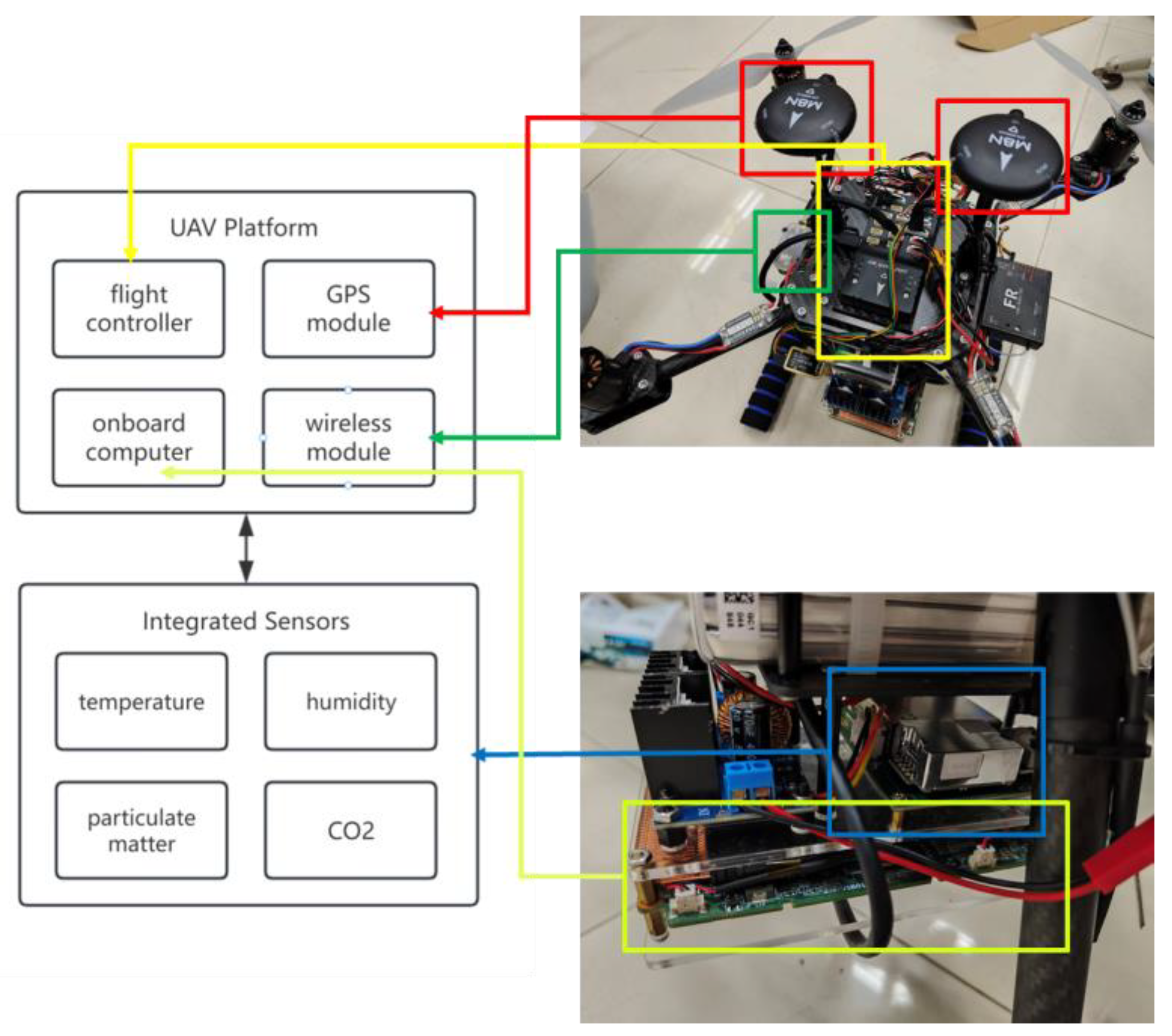
This study establishes a comprehensive UAV data collection system utilizing the PX4 open-source flight controller Pixhawk 6C (Holybro, Shenzhen, China), referred to as the flight controller as the core controller to assemble the UAV platform (Figure 1). The UAV is equipped with the CJ701 sensor (CJSL, Guangzhou, China), capable of collecting various data including CO₂, PM_2.5, temperature, and humidity. An onboard computer reads the numerical values of these data at 1 Hz via serial communication and concurrently connects to the flight controller through the Mavlink interface to retrieve and record the UAV’s current speed, position, attitude, and other data. The specific parameters of the sensors are shown in

Table 1. The specific parameters of sensors carried by the unmanned aerial vehicle (UAV).

Category	Measurement Resolution	Measurement Range	Measurement Accuracy
CO2	1 ppm	400~5000 ppm	±3% + 50 ppm or ±10%
PM2.5	1 µg/m3	0~999 µg/m3	±10% or ±10
Temperature	0.01 °C	−40~100 °C	±1 °C
Humidity	0.04%	0~100%	±3%RH
PM2.5	1 µg/m3	0~999 µg/m3	±10% or ±10

.

The sensors output collected data through I2C, UART, and other interfaces. The microcontroller reads and parses these data, then plots them. Subsequently, at a rate of 1 Hz, all sensor data are sent via serial communication to the onboard computer for processing.

2.2. Air Quality Data Correction Model

The movement of UAVs can induce airflow disturbances, affecting the accuracy of sensor data. To mitigate these errors, this study employs a motion compensation algorithm based on an Inertial Navigation System (INS), complemented by a Backpropagation (BP) neural network for sensor data correction. The INS integrates gyroscopes, accelerometers, and high-precision GPS to provide real-time motion state information of the UAV, including velocity, acceleration, and rotation angles.

Specifically, the BP neural network was employed to correct the disturbances in air quality measurements caused by the UAV’s airflow during flight. These disturbances arise from the complex and hard-to-quantify air currents generated by the UAV’s movement. Given that airflow is closely tied to the UAV’s dynamic behavior, we utilized internal flight data, capturing nine motion indicators: velocity and acceleration in the x, y, and z directions, as well as roll, yaw, and pitch angles.

The relationship between these motion parameters and the resulting sensor errors is highly non-linear, making it difficult to model using traditional physical approaches. Therefore, we selected the BP neural network for its robustness in handling non-linear relationships and its proven effectiveness in correcting measurement errors caused by external disturbances like airflow [20,21]. The BP neural network is particularly suited for this task because of its ability to model and learn the intricate dependencies between UAV motion and data distortions, thus enhancing the accuracy of the air quality measurements.

The network operates in two phases—forward propagation and backpropagation—continually optimizing its performance. During forward propagation, information flows smoothly from the input layer through the hidden layers to the output layer. In backpropagation, information flows in reverse to adjust network parameters, including weights (w) and biases (b), to achieve optimal prediction results. This operational process is distinctly divided into two phases, as depicted in Figure 2.

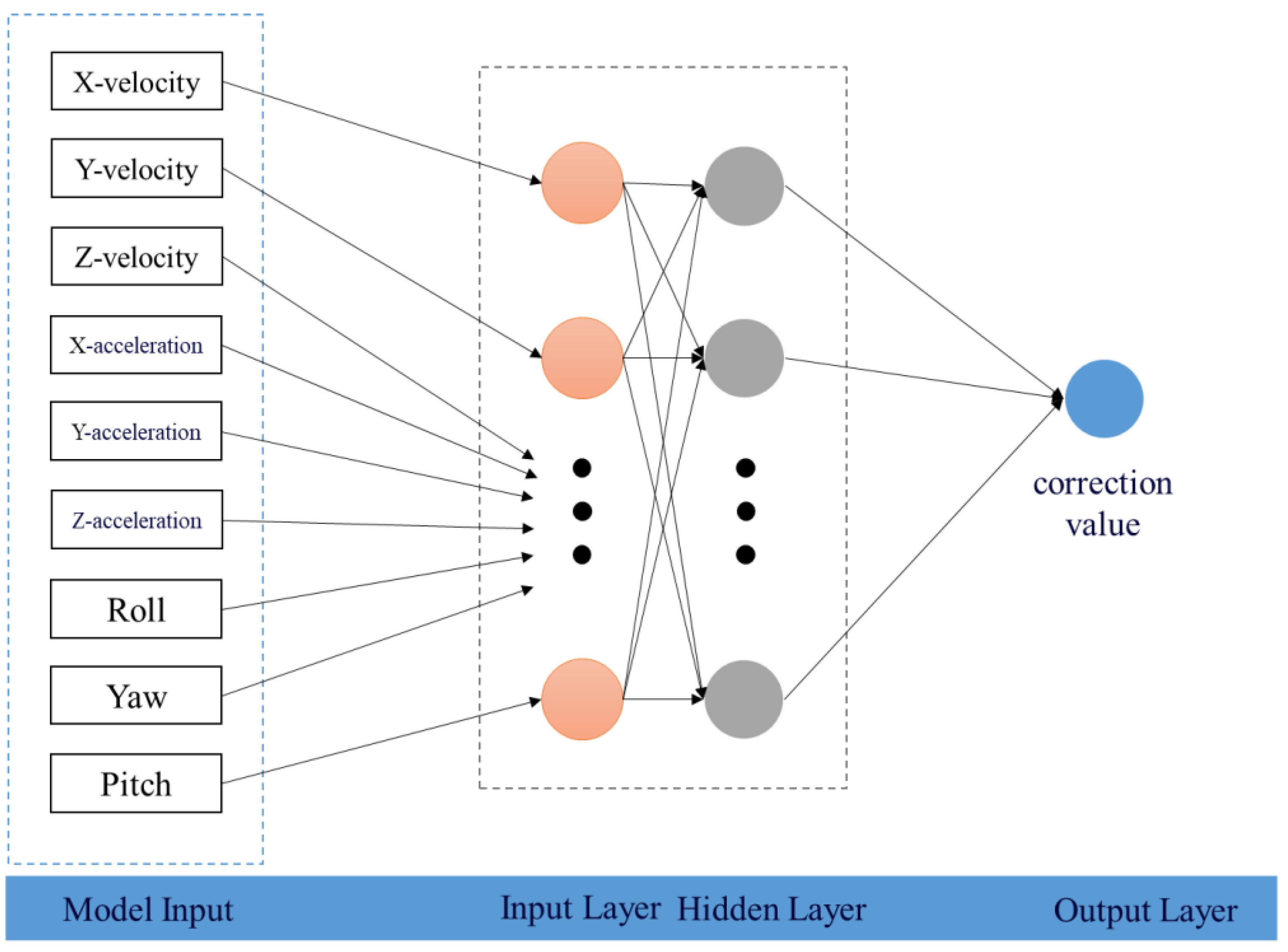
The core structure of this system consists of input, hidden, and output layers (as illustrated in Figure 3). In this study, the correction model specifically considers nine input factors: roll angle, yaw angle, and pitch angle, as well as velocities and accelerations in the x, y, and z directions. The output layer is responsible for providing corrected values of various air quality indices, which will be used for the dynamic correction of measured values.

For the UAV motion parameters used here, there are two main sources.

• Regarding acceleration and tilt angle, they come from the IMU sensor inside the flight control, specifically the following model: ICM-42688-P (TDK InvenSense, Tokyo, Japan). The main characteristics are listed in Table 2.

Table 2. Specifications of the ICM-42688-P imu sensor for acceleration and tilt angle measurements.

Parameter	Specification
GYRO Noise (mdps/rt-Hz)	2.8
GYRO Offset Temp Stability(mdps/°C)	±5
GVRO Range and Resolution	±2000 dps; 16/19-bits
ACCEL Noise (µg/rt-Hz)	AXY: 65; AZ: 70
ACCEL Range and Resolution	+16 g; 16/18-bits

Table 2. Specifications of the ICM-42688-P imu sensor for acceleration and tilt angle measurements.

Parameter	Specification
GYRO Noise (mdps/rt-Hz)	2.8
GYRO Offset Temp Stability(mdps/°C)	±5
GVRO Range and Resolution	±2000 dps; 16/19-bits
ACCEL Noise (µg/rt-Hz)	AXY: 65; AZ: 70
ACCEL Range and Resolution	+16 g; 16/18-bits

• The velocities in the x, y, and z directions come from the GPS carried by the aircraft, specifically signaled as with the Holybro M9N GPS (Holybro, Shenzhen, China), and the main characteristics are listed in

  Table 3. Specifications of the Holybro M9N GPS for velocity measurements in the x, y, and z directions.

  Parameter	Specification
  Receiver type	channel u-blox M9 engine GPS L1 C/A, QZSS L1 C/A/S, GLONASS L10F BeiDou B1l, Galileo E1B/C SBAS L1 C/A:WAAS, EGNOS, MSAS, GAGAN
  Nav. update rate	Up to 25 Hz (4 concurrent GNSS)
  Horizontal position accuracy	1.5 m CEP (with SBAS) 2.0 m CEP (without SBAS)

  .

2.3. Statistical Analysis

To investigate the impact of geographical spatial layout and structure on air quality, we employed two statistical methods: the two-sample F-test and two-way ANOVA, focusing on PM_2.5 concentration data. Initially, the two-sample F-test was applied to PM_2.5 measurements collected vertically at seven distinct locations, comparing the variance between each pair of locations. For the two-way ANOVA, altitude and location were defined as independent variables, while PM_2.5 concentration served as the dependent variable. Altitude was divided into five-meter intervals, and we calculated the mean and standard deviation of PM_2.5 concentration within each altitude interval across the seven locations. This approach allowed us to analyze the individual and interaction effects of altitude and location on PM_2.5 concentration, providing insights into the influence of spatial layout and structural factors on air quality.

2.4. Three-Dimensional Air Quality Data Spatial Interpolation Model

This method aims to transform discrete three-dimensional air quality scattered data into continuous voxel grid data using spatial interpolation techniques, facilitating visualization, analysis, and further scientific research on spatial distribution characteristics. This study utilizes point interpolation to voxel grid technology from SuperMap iDesktop 11i (2022) (V11.0.2) software, which combines advantages of spatial statistics and geographic information systems to effectively address interpolation challenges in three-dimensional spatial data. Each interpolation algorithm in ArcGIS (10.8) software has its own set of strengths and limitations [22]. However, given that the data collected in this experiment consist of non-uniformly distributed three-dimensional scattered points, which are significantly influenced by the geographical characteristics of the microenvironment, the Kriging interpolation method stands out as one of the most robust algorithms for handling such spatially heterogeneous data [23,24].

Kriging calculates the weights of known points around unknown points using covariance functions, semivariogram analysis, and theoretical variogram function models, and estimates the attribute values of unknown points through weighted averaging. This method fully considers the three-dimensional distribution characteristics and spatial correlations of data in three-dimensional space, suitable for the interpolation analysis of complex terrain and environmental factors [25].

Specifically, three-dimensional Kriging interpolation can be described as follows:

Semivariogram computation: The semivariogram function $\gamma \left(h\right)$ describes the spatial correlation between two points. For three-dimensional data points $\left(x_i,y_i,z_i\right)$ and $\left(x_j,y_j,z_j\right)$, their distance $h$ can be expressed as follows [22]:

$$\begin{array}{c}h=\sqrt{{\left(x_i-x_j\right)}^2+{\left(y_i-y_j\right)}^2+{\left(z_i-z_j\right)}^2}\end{array}$$

(1)

The semivariogram function $\gamma \left(h\right)$ typically employs empirical formulas or theoretical models such as exponential, Gaussian, or spherical models.

Covariance function and variogram model: Based on the semivariogram function, the covariance function $C\left(h\right)$ and variogram model are constructed to define the spatial relationship between known and unknown points.

Kriging coefficients are computed by solving the Kriging coefficient matrix equation, which determines the weight ${\mathsf{\lambda }}_{\mathrm{i}}$ for each known point. For a target point $\left(x_0,y_0,z_0\right)$, the estimated attribute value $t_0$ can be expressed as follows:

$$\begin{array}{c}{t}_0={\displaystyle \sum _{i=1}^n}{\mathsf{\lambda }}_i{t}_i\end{array}$$

(2)

where $t_i$ represents the attribute value of the known point $\left(x_i,y_i,z_i\right)$, and ${\mathsf{\lambda }}_{\mathrm{i}}$ denotes the corresponding weight coefficient, determined by the following system of linear equations:

$$\begin{array}{c}\left\{\begin{array}{l}{\displaystyle \sum _{i=1}^n} {\lambda }_i\gamma \left(\right(x_i,y_i,z_i),(x_j,y_j,z_j\left)\right)+\mu =\gamma \left(\right(x_0,y_0,z_0),(x_j,y_j,z_j\left)\right),\hspace{0.25em}\hspace{0.25em}\hspace{0.25em}\hspace{0.25em}j=\mathrm{1,2},\dots ,n\\ {\displaystyle \sum _{i=1}^n} {\lambda }_i=1\end{array}\right.\end{array}$$

(3)

where $\mu$ is the Lagrange multiplier used to ensure that the sum of the weight coefficients equals 1.

This study interpolates three-dimensional air quality scattered data with 60 interpolation layers, each layer accurate to 1 m.

3. Results

3.1. Study Area Overview

The Science and Technology Teaching Area of Guangzhou University (23.11667° N, 113.25000° E) was chosen as the measurement site for this study. As shown in Figure 4, the layout of the teaching area is as follows:

To the west, from north to south, there are an unnamed building under construction, Teaching Building A, and Laboratory Building A. In the center is Laboratory Building B, which is the main hub for science and engineering laboratories, equipped with extensive experimental facilities. Additionally, the floor inside the atrium of Laboratory Building B is undergoing large-scale construction, which may also significantly impact air quality. East of the laboratory buildings is the canteen, with lawns to the east, the library to the northeast, and the central square surrounding the central lake on the west side.

Overall, the southwest and west sides of the teaching area feature dense trees and patches of lawn between the buildings, while the eastern area is characterized by flat and open squares and lawns with sparse vegetation. This unique microenvironment structure and distribution provide an ideal background for this study.

Recently, the study area has experienced continuous rainy weather, with significant precipitation and winds blowing from the ocean towards the inland. These weather phenomena have had a notable impact on the air quality in the study area.

3.2. Data Collection and Correction Results

3.2.1. Data Collection

To minimize the influence of wind on pollutant dispersion and focus on the relationship between microenvironment characteristics and air quality, data collection was conducted during periods of relatively calm, low-wind conditions. This ensured that the variations in air quality indices observed in the study primarily reflected the effects of local geographical features and structures, rather than external meteorological factors.

• Training Data Collection

To construct the neural network correction model, data necessary for training were first collected. The UAV dynamically measured a series of data points in various flight attitudes, while simultaneously statistically measuring using sensors at the same location to obtain reference values. The difference (i.e., correction values) between these data sets served as the dependent variable for model training, while UAV flight attitudes, speed, and other parameters served as independent variables. By training the BP neural network, the aim was to reveal the relationships between these parameters and the correction values.

• Testing Data Collection

Testing data collection involved two methods: vertical collection and fill-in collection. Vertical collection consisted of the UAV ascending uniformly from ground level to 60 m, continuously measuring air quality. Fill-in collection involved the UAV randomly flying in three-dimensional space to ensure the even distribution of sampling points.

All data were collected in the afternoon (16:00–18:00) from May to June 2024, primarily under stable weather conditions with a higher humidity, often cloudy or rainy.

3.2.2. Correction Results

Table 4. Performance of the BP neural network correction model.

Loss Function	CO2	Temperature	PM2.5	Humidity
MSE	0.039112	0.014064	0.031388	0.049695
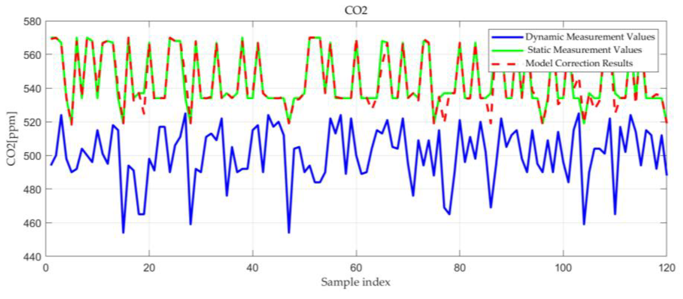
R2	0.9595	0.98471	0.9618	0.95406

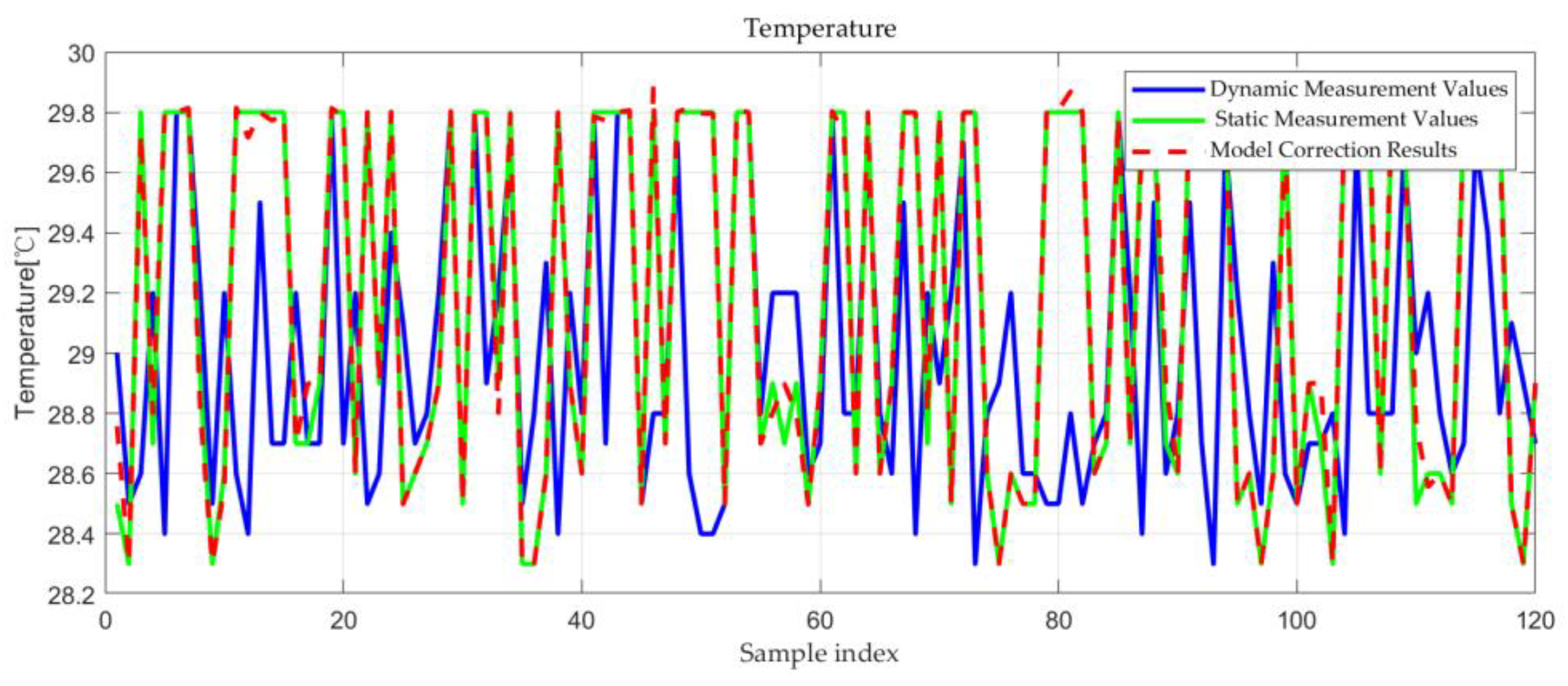
summarizes the loss function of the BP neural network model, and Figure 5 illustrates the relationship between dynamic measurement values of the UAV and the model-corrected values with static measurement values. According to Table 4, the mean squared errors of the BP neural network models for the four air quality indices are all less than 0.1, and the coefficient of determination R² exceeds 90%. From Figure 5, Figure 6, Figure 7 and Figure 8, it is evident that there is a significant deviation between the model-corrected values and the dynamic measurement values, whereas they align closely with the static measurement values overall. These results indicate that the BP neural network model performs well in terms of fitting, accurately capturing patterns within the data. In these figures (Figure 5, Figure 6, Figure 7 and Figure 8), the green line represents the static measurement values, which are the control group data measured by the sensors in an ideal stationary state. The blue line represents the dynamic measurement values, which are the data measured by the sensors mounted on the UAV during flight in the same series of positions. The red dashed line represents the model correction results, which is the sum of the dynamic measurement values and the corrected values predicted by the neural network model.

3.3. Analysis of Vertical Distribution of Air Quality

In this study, vertical profiles of air quality data were corrected and plotted as line graphs, and variations with altitude were analyzed in relation to the specific geographical microenvironment characteristics of each collection point.

• Collection Point 1 was located at the center of a lake, surrounded by a large expanse of water and sparse tree vegetation, providing a unique water-influenced microenvironment.
• Collection Point 2 was situated in the central area of a square, with sparse tree vegetation distributed on both its east and west sides, creating an open, less vegetated environment.
• Collection Point 3, to the east of Laboratory Building A, was surrounded by dense vegetation and nearby buildings, offering a more enclosed, densely vegetated microenvironment.
• Collection Point 4 lay between Laboratory Building B and the Administrative Building. To its south, there was an asphalt road lined with dense vegetation and a small water body along the roadside, combining man-made surfaces with natural elements.
• Collection Point 5 was in the southwest of the educational zone, surrounded mainly by sparse trees, water bodies, and some bare ground, with an asphalt road lying to the southwest.
• Collection Point 6 was located in the central part of the educational zone, surrounded by dense tree vegetation, with the ground covered in lawn soil, reflecting a primarily vegetated area.
• Collection Point 7 was on the east side of the educational zone, featuring a spacious lawn area with fewer trees. The perimeter of the lawn was covered with impermeable surfaces, representing a more open microenvironment with significant impervious ground cover.

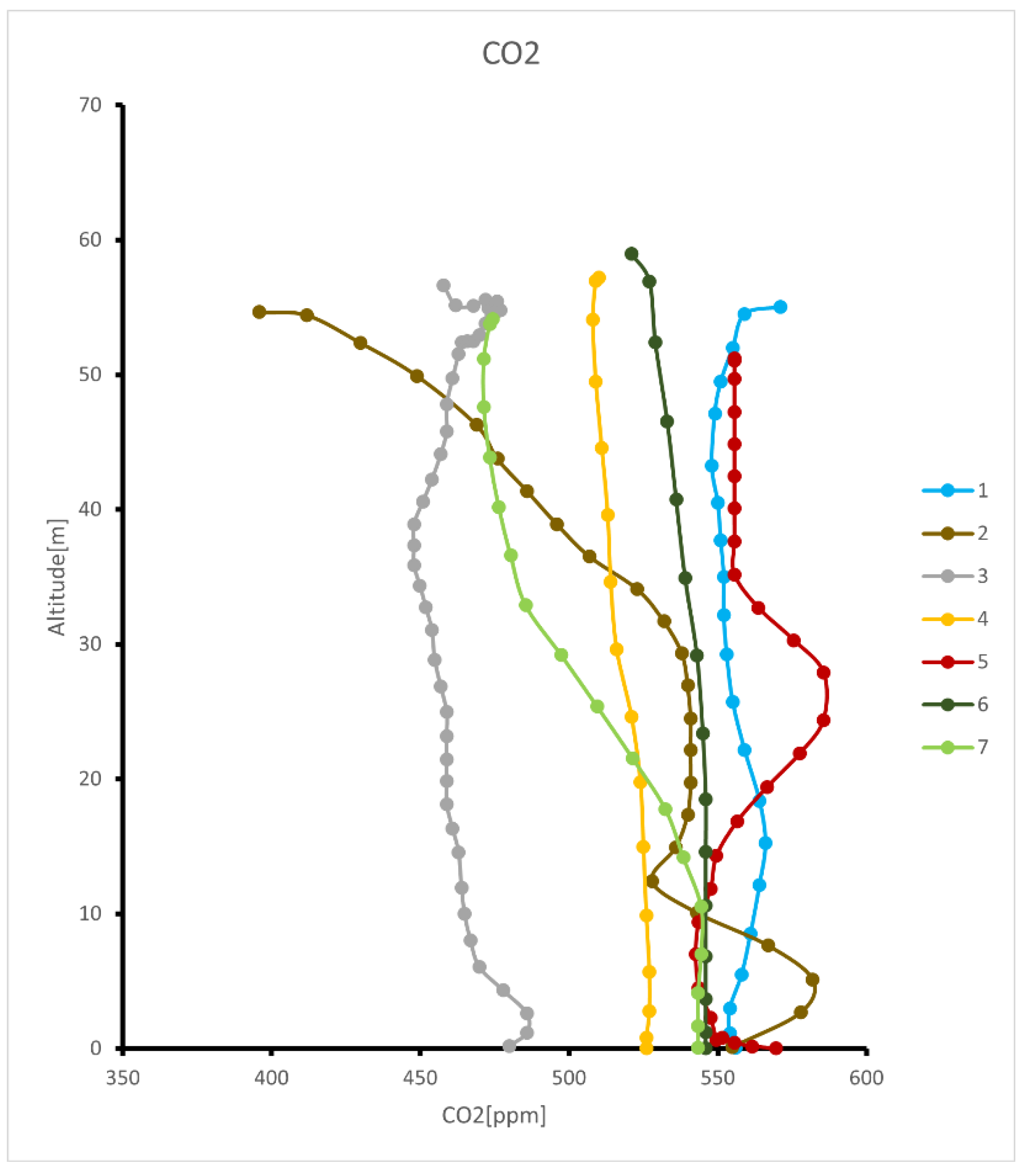
As shown in Figure 9, the CO₂ concentration is lowest at Point 3 and highest at Point 5. With increasing altitude, significant reductions in CO₂ concentration are observed at Point 2 in the square area and Point 7 in the lawn area. The decrease in CO₂ concentration at Point 2 is particularly steep, surpassing the previously lowest concentration at Point 3 at an altitude of approximately 50 m, becoming the new low point. This reflects the promoting effect of open areas on the vertical dispersion of CO₂.

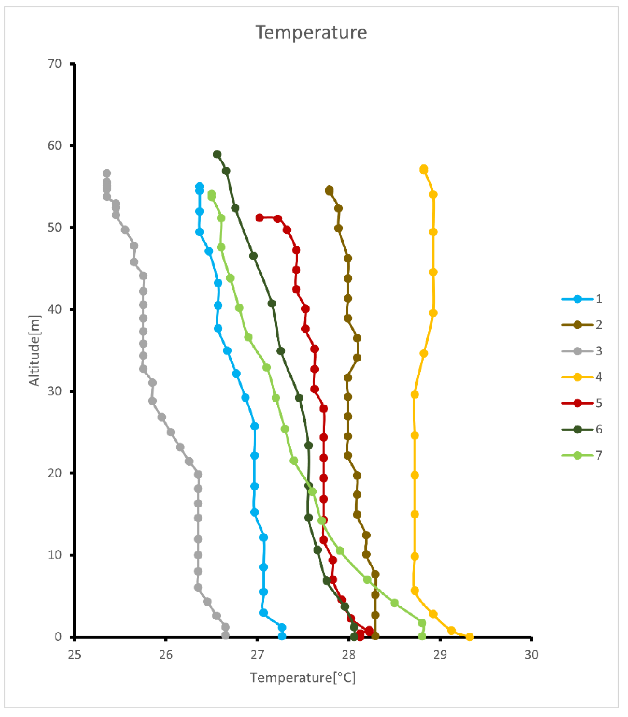
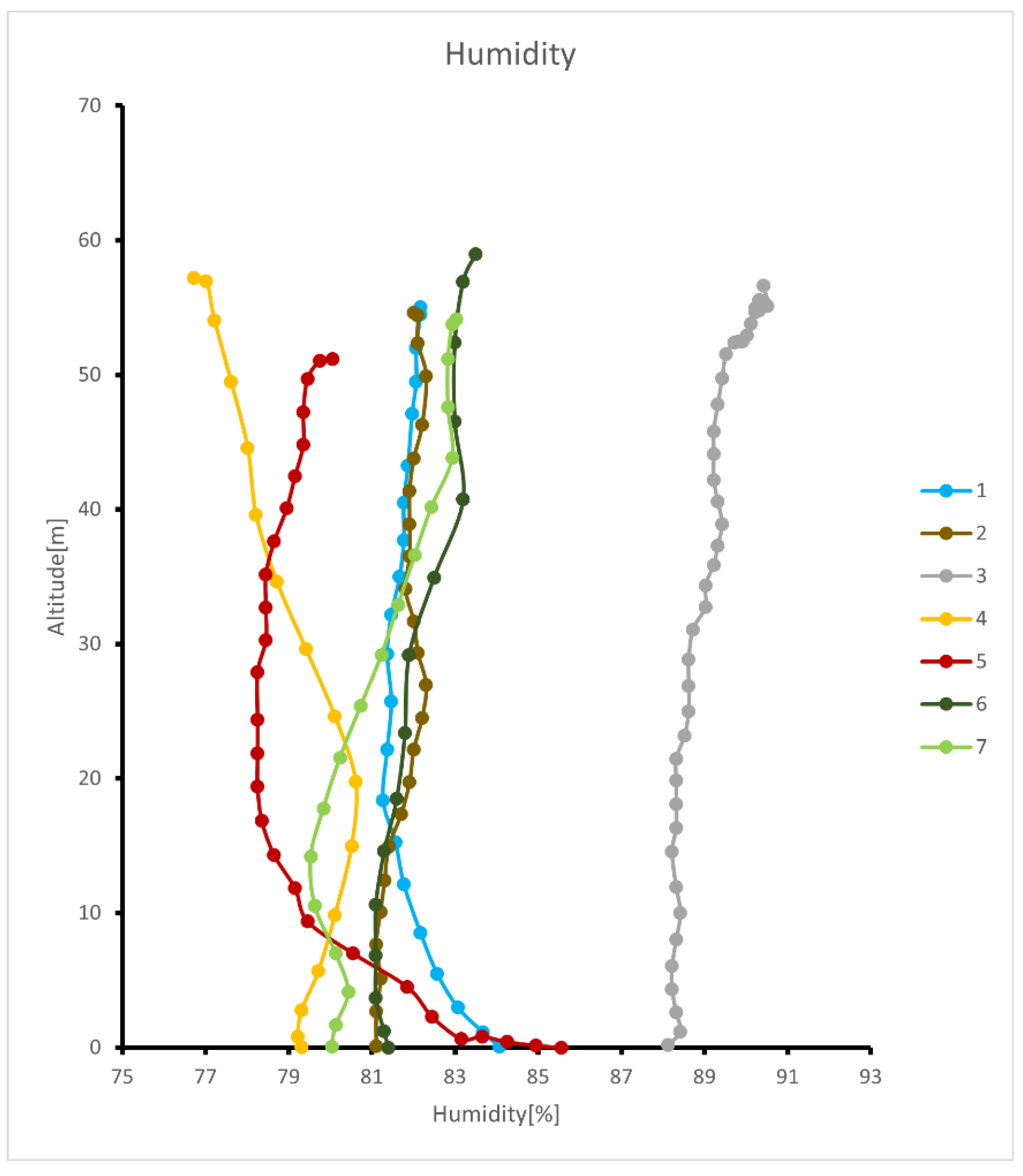
As shown in Figure 10, with increasing altitude, the temperature at various points exhibits a decreasing trend, which aligns with the common atmospheric phenomenon known as the lapse rate [26]. It can be observed that the temperature at Point 3 consistently remains lower than at other locations, while Point 4 consistently shows the highest temperature levels. This is in direct contrast to the humidity trends shown in Figure 11, where the humidity at Point 3 is significantly higher than at other points, and Point 4 has the lowest humidity. Except for Points 4 and 5, the humidity at the other locations increases with altitude. This is because lower temperatures at higher altitudes reduce the air’s capacity to hold water vapor, thereby increasing relative humidity [27,28].

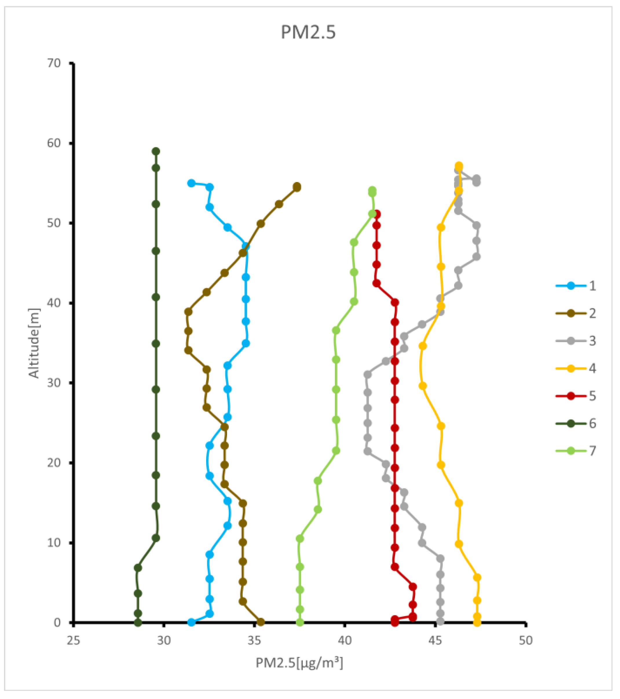
As shown in Figure 12, PM_2.5 concentrations are generally higher at Point 3 near Laboratory Building B, which is under construction, and Point 4 near Laboratory Building A. This indicates that dust from construction activities and the operation of large electronic experimental equipment increase particulate matter levels in the surrounding air. At Point 6 where vegetation is dense, PM_2.5 levels are significantly lower than at other monitoring points, demonstrating the effective filtering and adsorption of airborne particles by vegetation.

The F-test results, with p-values below 0.05 for all pairwise comparisons among the seven sampling points, indicate statistically significant differences in PM_2.5 concentration variance between each location pair. This suggests that the geographical layout and structural differences among the sampling points substantially influence PM_2.5 levels, underscoring the impact of spatial configuration on air quality variations. Based on the results of the two-way ANOVA (

Table 5. Two-way ANOVA location and altitude and their interaction on PM_2.5 concentrations.

Source	Type III Sum of Squares	df	Mean Square	F	Sig
Altitude	37.416	10	3.742	2.593	<0.01
Location	31,870.211	6	5311.702	3681.345	<0.01
Altitude × Location	346.246	60	5.771	4	<0.01

), both “location” and “altitude” exhibit significant effects on PM_2.5 concentrations. The location effect, with a significance level below 0.01, indicates substantial differences in PM_2.5 values across sampling points, suggesting a pronounced spatial variation in PM_2.5 concentrations among different geographic locations, consistent with the F-test findings. Additionally, altitude shows a significance level below 0.01, demonstrating that PM_2.5 concentrations vary significantly with height. The significant interaction effect between location and altitude (p < 0.01) suggests that the influence of altitude on PM_2.5 concentrations varies across different locations. This interaction provides key insights for further investigation into the spatial distribution and vertical variation patterns of PM_2.5 concentrations.

Based on the results from Duncan’s post hoc test (

Table 6. Mean and standard deviation of PM_2.5 concentrations across different geographic locations and altitudes, along with Duncan’s post hoc test results for significant differences. For each column, different lowercase letters indicate significantly different at p  ≤  0.01. For each row, different capital letters indicate significant differences at p ≤ 0.01.

Altitude [m]	Location
	Point 1	Point 2	Point 3	Point 4	Point 5	Point 6	Point 7
0~5	32.72 ± 1.23 bcF	34.55 ± 2.1 abcE	46.37 ± 0.32 abB	47.91 ± 0.52 abcA	42.45 ± 0.48 aC	28.46 ± 0.88 dG	36.81 ± 1.64 dD
5~10	33.92 ± 1.07 aE	33.85 ± 1.08 bcE	46.12 ± 0.31 abcB	47.48 ± 0.3 bcA	41.75 ± 0 cC	28.23 ± 0.27 dF	37.18 ± 1.09 cdD
10~15	33.35 ± 0.87 abE	33.15 ± 2.04 bcE	45.84 ± 0.64 abcdB	47.31 ± 0 cA	42 ± 0.29 bcC	28.56 ± 0 cdF	36.76 ± 1.19 dD
15~20	32.95 ± 0.93 bcE	32.85 ± 3.13 bcE	44.93 ± 1.12 deB	47.31 ± 0.47 cA	42.25 ± 0.33 abC	28.89 ± 0.27 cF	37.51 ± 0.82 bcdD
20~25	32.52 ± 0.67 bcE	33.92 ± 3.59 bcE	44.55 ± 1.75 eB	47.64 ± 0.54 bcA	42.25 ± 0.33 abC	29.56 ± 0.47 bF	37.85 ± 0.54 abcD
25~30	32.69 ± 0.73 bcE	33.1 ± 4.18 bcE	45.43 ± 1.85 bcdeB	47.31 ± 0.82 cA	42.25 ± 0.24 abC	29.89 ± 0.54 bF	37.18 ± 0.54 cdD
30~35	32.95 ± 0.8 bcE	33.35 ± 3.43 bcE	45.12 ± 1.73 cdeB	47.31 ± 0.82 cA	42.25 ± 0.33 abC	29.89 ± 0.54 bF	37.85 ± 0.54 abcD
35~40	32.95 ± 0.64 bcE	32.02 ± 3.2 cE	46.67 ± 0.6 aB	48.31 ± 0.82 aA	42 ± 0.29 bcC	30.56 ± 0 aF	37.85 ± 0.54 abcD
40~45	33.15 ± 0.81 abcF	34.1 ± 0.87 bcE	46.52 ± 0.41 abB	48.31 ± 0.82 aA	41.35 ± 0.37 dC	29.56 ± 0.47 bG	38.01 ± 0.33 abD
45~50	32.97 ± 0.68 bcF	34.95 ± 0.37 abE	46.39 ± 1.45 abB	47.98 ± 0.72 abA	40.75 ± 0 eC	28.89 ± 0.27 cG	38.18 ± 0.27 abD
50~55	32.41 ± 0.74 cF	36.85 ± 0.41 aE	46.97 ± 1.34 aB	47.71 ± 0.37 abcA	40.75 ± 0 eC	28.56 ± 0 cdG	38.51 ± 0 aD

), significant differences in PM_2.5 concentrations were observed among most location points at the same altitude, as indicated by the distinct uppercase letter labels across the seven points. This suggests that PM_2.5 levels vary significantly across the seven locations, likely due to differences in geographic layout. However, between Points 1 and 2 at the 10 to 40 m range, no significant differences were detected in PM_2.5 concentrations, which may result from the similar, open spatial layout of these points, leading to comparable impacts on PM_2.5 dispersion.

For the same location points at varying altitudes, PM_2.5 concentrations generally showed no significant differences across heights, with a few notable exceptions. Points 3 and 4 displayed significant differences in PM_2.5 concentrations above and below the 35 m mark, while Point 5 exhibited similar variation around the 40 m mark. This pattern may be due to the presence of tall buildings and dense vegetation near these points, where similar geographic layouts likely influence air circulation and particulate matter distribution differently above and below certain heights.

3.4. Spatial Interpolation Results and 3D Visualization

The results of the visualization and analysis by overlaying the 3D air quality distribution model with the oblique photography model are shown in Figure 9, Figure 10, Figure 11 and Figure 12.

Figure 13 illustrates that CO₂ concentrations near the ground are higher in densely vegetated areas. This is likely due to rainwater promoting soil microbial activity and plant respiration. Conversely, CO₂ concentrations are lower in plaza and water areas, possibly due to their relatively open nature and good ventilation conditions, which facilitate CO₂ diffusion. Concentrations gradually decrease with increasing height.

Figure 14 depicts the temperature distribution. Temperatures are relatively higher above water bodies and vegetation, while they are lower above the plaza area. This pattern may be attributed to the higher thermal capacity of water bodies and vegetation, allowing them to store and slowly release heat. Additionally, although water evaporation typically lowers ambient temperatures, high humidity slows down the evaporation rate, thereby weakening this cooling effect.

Figure 15 reveals the characteristics of humidity distribution, which is inversely correlated with temperature. Humidity levels are generally lower near the ground but increase gradually with height. Above the boundary between water bodies and vegetation, humidity is relatively higher, likely due to vegetation transpiration and atmospheric mixing effects.

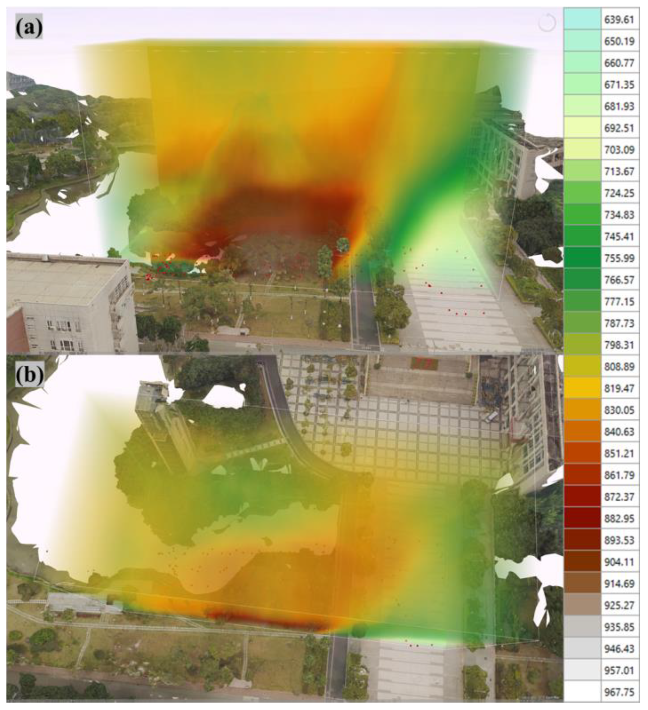
Figure 16 displays the distribution of PM_2.5 concentrations. PM_2.5 concentrations are lower above the plaza area, while they are higher above water bodies and vegetation areas, increasing with height. This may result from a combination of high humidity and restricted air movement, leading to particle accumulation in these areas. In contrast, particles are less likely to accumulate in the more open and well-ventilated plaza areas.

4. Discussion

This study successfully demonstrates the capabilities of a novel UAV air quality monitoring platform, effectively correcting sensor data through controlled experiments and a BP neural network algorithm. By eliminating the influence of drone motion on sensor readings, we have established a reliable methodology for air quality data collection. Our results indicate that drone flight significantly impacts sensor data; however, this effect can be accurately predicted and corrected, showcasing the robustness of our correction model across various scenarios.

Unlike existing UAV platforms, which often utilize commercially available drones with limited data accessibility, our custom-designed system enables direct access to critical internal flight data, including precise spatial coordinates and real-time motion parameters. This capability allows for more accurate corrections of sensor data, thereby enhancing the overall reliability of air quality measurements. By addressing the limitations of standard UAVs, our platform sets a new benchmark for precision in drone-based environmental monitoring.

Our comprehensive analyses of air quality indicators, particularly CO₂ concentration, relative humidity, temperature, and PM_2.5 density, reveal complex variations with height, diverging significantly from traditional macro-scale studies. For instance, we observed that regions with dense vegetation exhibit higher CO₂ levels, suggesting that prolonged overcast conditions favor plant respiration over photosynthesis [29,30]. The phenomenon of elevated CO₂ levels in densely vegetated areas highlights the necessity of integrating local climatic characteristics and building layouts when designing urban vegetation strategies. In regions characterized by extended cloudy or rainy conditions, or where buildings are densely clustered and tall, excessive planting of vegetation could lead to the accumulation of CO₂ and other pollutants [31]. This is particularly concerning when sunlight exposure is limited, as reduced photosynthesis can hinder the natural cleansing effects of vegetation, resulting in stagnant air and increased humidity levels. Such conditions may impair air circulation and foster the proliferation of soil microorganisms, posing health risks to local populations.

In the results of statistical analyses, significant variations in PM_2.5 concentrations were observed across different geographic locations, even within this small-scale area. However, PM_2.5 levels showed no overall significant difference with height, except in regions characterized by clusters of tall, dense buildings and vegetation. At these specific sites, PM_2.5 concentrations exhibited significant differences above and below certain fixed heights, likely due to the impact of structural features on air circulation patterns [32]. This suggests that while altitude alone may not consistently influence PM_2.5 distribution, the presence of concentrated vertical structures can create distinct particulate variations at certain height thresholds, underscoring the nuanced role of geographic layout in air quality within microenvironments.

Moreover, the three-dimensional distribution models generated through our UAV platform indicate that air quality dynamics at the microenvironment scale are intricately linked to geographic and structural features. For example, the correlation between high humidity and elevated PM_2.5 concentrations in areas with extensive electronic equipment underscores the necessity for targeted monitoring strategies in urban planning and public health initiatives [33,34]. Maintaining a safe distance between these pollution sources and residential or workplace environments is essential to mitigate air quality degradation and its associated health impacts.

Interestingly, we found that areas with dense vegetation and water bodies can exhibit elevated levels of CO₂ and PM_2.5, contrary to common assumptions that these areas provide cleaner air. This suggests a complex interplay of environmental factors, such as stagnant air and hygroscopic particle growth, which could inform future research on air quality management in urban settings [28,35,36,37].

In summary, our UAV platform not only enhances the accuracy of air quality measurements but also provides novel insights into the behavior of air pollution variables within urban microenvironments. By contrasting our findings with the existing literature, we demonstrate a significant advancement in understanding air quality dynamics, paving the way for future studies and practical applications in environmental science.

5. Conclusions

This study conducted comprehensive air quality measurements across various monitoring points on campus using drones equipped with advanced sensor systems. The application of a BP neural network algorithm effectively corrected the collected data, significantly mitigating the influences of drone movements—an improvement over traditional monitoring methods that often suffer from static positioning and limited data collection capabilities.

By employing drones, this research enabled real-time, high-resolution data collection across a microenvironment, addressing the limitations of conventional ground-based monitoring stations, which can be hampered by their fixed locations and inability to capture spatial variations in pollutant concentrations. Additionally, the flexibility of drone deployment allows for targeted monitoring in areas that may be challenging to access otherwise.

The analysis of air quality indicators—such as CO₂ concentration, humidity, temperature, and PM_2.5 density—revealed diverse patterns of variation. Notably, areas characterized by dense buildings, ongoing construction, and large electronic equipment demonstrated significantly elevated PM_2.5 levels. Conversely, high humidity and relatively enclosed spaces impeded air circulation, resulting in poor air quality, which poses potential health risks upon prolonged exposure. Geographic layout significantly impacts PM_2.5 distribution in microenvironments, with notable height-based variations occurring particularly in areas with dense, tall structures.

This study highlights the potential of utilizing drones in future air quality assessments, as they offer a novel approach to understanding the dynamics of microenvironments. Furthermore, these findings provide crucial insights for urban planning and environmental management, emphasizing the need for adaptive strategies to improve air quality in densely populated areas. Overall, this innovative use of drone technology combined with advanced data processing techniques represents a significant advancement in the field of environmental monitoring.

Furthermore, the integration of detailed 3D air quality information into urban layout and building design could significantly enhance sustainable development efforts. For instance, understanding air pollutant distribution in relation to urban structures may help optimize building orientation and ventilation systems to reduce pollution exposure. In addition, such 3D insights can guide the strategic placement of green infrastructure (e.g., parks, trees) and blue infrastructure (e.g., water bodies) to mitigate pollution and manage urban heat islands. This data-driven approach would support the design of healthier, more resilient cities by leveraging natural elements for air quality improvement and better urban climate regulation.

However, despite the advantages of UAV techniques, certain limitations should be acknowledged. The limited battery life and payload capacity of drones can restrict the duration of monitoring and the range of sensors that can be carried. Additionally, drones are sensitive to environmental conditions such as wind speed and turbulence, which may influence data accuracy, particularly in regions with complex topography. Furthermore, the cost of high-quality sensor-equipped drones and the need for skilled operators could limit the widespread application of this technology. Addressing these limitations in future research could enhance the reliability and accessibility of UAV-based air quality monitoring.

References

- Iungman, T.; Khomenko, S.; Barboza, E.P.; Cirach, M.; Gonçalves, K.; Petrone, P.; Nieuwenhuijsen, M. The impact of urban configuration types on urban heat islands, air pollution, CO2 emissions, and mortality in Europe: A data science approach. Lancet Planet. Health 2024, 8, e489–e505. [Google Scholar] [CrossRef] [PubMed]
- Yang, Q.; Huang, X.; Tang, Q. The footprint of urban heat island effect in 302 Chinese cities: Temporal trends and associated factors. Sci. Total Environ. 2019, 655, 652–662. [Google Scholar] [CrossRef] [PubMed]
- Yin, J.; Wu, X.; Shen, M.; Zhang, X.; Zhu, C.; Xiang, H.; Shi, C.; Guo, Z.; Li, C. Impact of urban greenspace spatial pattern on land surface temperature: A case study in Beijing metropolitan area, China. Landsc. Ecol. 2019, 34, 2949–2961. [Google Scholar] [CrossRef]
- Vujovic, S.; Haddad, B.; Karaky, H.; Sebaibi, N.; Boutouil, M. Urban Heat Island: Causes, Consequences, and Mitigation Measures with Emphasis on Reflective and Permeable Pavements. CivilEng 2021, 2, 459–484. [Google Scholar] [CrossRef]
- Ramberg-Pihl, N.; Barrowman, S.; Bhajan, L.; Cronin-Golomb, O.; Gambino, C. Quantifying Changes in Urban Albedo with NASA Earth Observations to Reduce the Urban Heat Island Effect in Cambridge, Massachusetts. In Proceedings of the AGU Fall Meeting, San Francisco, CA, USA, 14–18 December 2020. [Google Scholar]
- Wang, S.; Ma, Y.; Wang, Z.; Wang, L.; Chi, X.; Ding, A.; Zhang, Y. Mobile Monitoring of Urban Air Quality at High Spatial Resolution by Low-Cost Sensors: Impacts of COVID-19 Pandemic Lockdown. Atmos. Chem. Phys. 2021, 21, 7199–7215. [Google Scholar] [CrossRef]
- Peng, Z.R.; Wang, D.S.; Wang, Z.Y.; Gao, Y.; Lu, S.J. A study of vertical distribution patterns of PM concentrations based on ambient monitoring with unmanned aerial vehicles: A case in Hangzhou, China. Atmos. Environ. 2015, 123, 357–369. [Google Scholar] [CrossRef]
- Zhang, Y.; Dong, T.; Liu, Y. Design of meteorological element detection platform for atmospheric boundary layer based on UAV. Int. J. Aerosp. Eng. 2017, 2017, 1831676. [Google Scholar] [CrossRef]
- Xiaoyu, S.; Yuanhang, L.; Ligang, C.; Xin, Z.; Guoli, M. Research and Design of UAV Environmental Monitoring System. In Advanced Hybrid Information Processing: Proceedings of the 4th EAI International Conference, ADHIP 2020, Binzhou, China, 26–27 September 2020; Proceedings, Part I; Springer International Publishing: Berlin/Heidelberg, Germany, 2021; pp. 11–17. [Google Scholar]
- Villa, T.F.; Salimi, F.; Morton, K.; Morawska, L.; Gonzalez, F. Development and validation of a UAV based system for air pollution measurements. Sensors 2016, 16, 2202. [Google Scholar] [CrossRef]
- Peng, Y.; Ye, J.; Zhang, L.; Nie, C.; Ni, H.; Zhang, A. Research on 3D Air Quality Monitoring by UAV. Surv. Mapp. Sci. 2017, 42, 154–157+170. (In Chinese) [Google Scholar]
- Lu, S.; Wang, D.; Li, X.; Wang, Z.; Peng, Z.; Gao, Y. 3D Distribution Monitoring of Fine Particles Based on UAV Platform. Sci. Technol. Eng. 2017, 17, 94–100. (In Chinese) [Google Scholar]
- Connor, D.T.; Martin, P.G.; Smith, N.T.; Payne, L.; Hutson, C.; Payton, O.D.; Yamashiki, Y.; Scott, T.B. Application of airborne photogrammetry for the visualization and assessment of contamination migration arising from a Fukushima waste storage facility. Environ. Pollut. 2018, 234, 610–619. [Google Scholar] [CrossRef] [PubMed]
- Jaroń, A.; Borucka, A.; Deliś, P.; Sekrecka, A. An Assessment of the Possibility of Using Unmanned Aerial Vehicles to Identify and Map Air Pollution from Infrastructure Emissions. Energies 2024, 17, 577. [Google Scholar] [CrossRef]
- Zhu, Z.; Chen, B.; Zhao, Y.; Ji, Y. Multi-sensing paradigm based urban air quality monitoring and hazardous gas source analyzing: A review. J. Saf. Sci. Resil. 2021, 2, 131–145. [Google Scholar] [CrossRef]
- Singh, D.; Dahiya, M.; Kumar, R.; Nanda, C. Sensors and systems for air quality assessment monitoring and management: A review. J. Environ. Manag. 2021, 289, 112510. [Google Scholar] [CrossRef] [PubMed]
- Peng, J.; Zhang, P. Velocity Prediction Method of Quadrotor UAV Based on BP Neural Network. In Proceedings of the 2020 International Symposium on Autonomous Systems (ISAS), Guangzhou, China, 23–28 December 2020; IEEE: New York, NY, USA, 2020; pp. 23–28. [Google Scholar]
- Blond, N.; Bel, L.; Vautard, R. Three-dimensional ozone data analysis with an air quality model over the Paris area. J. Geophys. Res. Atmos. 2003, 108, D23. [Google Scholar] [CrossRef]
- Kalo, M.; Zhou, X.; Li, L.; Tong, W.; Piltner, R. Sensing air quality: Spatiotemporal interpolation and visualization of real-time air pollution data for the contiguous United States. In Spatiotemporal Analysis of Air Pollution and Its Application in Public Health; Elsevier: Amsterdam, The Netherlands, 2020; pp. 169–196. [Google Scholar]
- Wang, Z.; Xie, C.; Liu, B.; Jiang, Y.; Li, Z.; Tai, H.; Li, X. Self-adaptive temperature and humidity compensation based on improved deep BP neural network for NO2 detection in complex environment. Sens. Actuators B Chem. 2022, 362, 131812. [Google Scholar] [CrossRef]
- Patra, J.C.; Chakraborty, G.; Meher, P.K. Neural-network-based robust linearization and compensation technique for sensors under nonlinear environmental influences. IEEE Trans. Circuits Syst. I Regul. Pap. 2008, 55, 1316–1327. [Google Scholar] [CrossRef]
- Cressie, N. Statistics for Spatial Data; John Wiley & Sons: New York, NY, USA, 2015. [Google Scholar]
- Dupuy, R.; Makar, A. Analysis of digital sea bottom models generated using ENC data. Annu. Navig. 2011, 18, 27–36. [Google Scholar]
- Alcaras, E.; Amoroso, P.P.; Parente, C. The Influence of Interpolated Point Location and Density on 3D Bathymetric Models Generated by Kriging Methods: An Application on the Giglio Island Seabed (Italy). Geosciences 2022, 12, 62. [Google Scholar] [CrossRef]
- Deutsch, C.; Deutsch, J. Introduction to Choosing a Kriging Plan. Geostat. Lessons 2015. Available online: https://geostatisticslessons.com/lessons/introkrigingplan (accessed on 22 September 2024).
- Hwang, H.; Lee, J.E.; Shin, S.A.; You, C.R.; Shin, S.H.; Park, J.-S.; Lee, J.Y. Vertical Profiles of PM2.5 and O3 Measured Using an Unmanned Aerial Vehicle (UAV) and Their Relationships with Synoptic- and Local-Scale Air Movements. Remote Sens. 2024, 16, 1581. [Google Scholar] [CrossRef]
- Dong, D.; Huang, G.; Qu, X.; Tao, W.; Fan, G. Temperature Trend–Altitude Relationship in China during 1963–2012. Theor. Appl. Climatol. 2015, 122, 285–294. [Google Scholar] [CrossRef]
- Zebende, G.F.; Brito, A.A.; Silva Filho, A.M.; Castro, A.P. ρDCCA Applied between Air Temperature and Relative Humidity: An Hour/Hour View. Phys. A Stat. Mech. Its Appl. 2018, 494, 17–26. [Google Scholar] [CrossRef]
- Matteucci, M.; Gruening, C.; Ballarin, I.G.; Seufert, G.; Cescatti, A. Components, drivers and temporal dynamics of ecosystem respiration in a Mediterranean pine forest. Soil Biol. Biochem. 2015, 88, 224–235. [Google Scholar] [CrossRef]
- Wright, I.J.; Reich, P.B.; Atkin, O.K.; Lusk, C.H.; Tjoelker, M.G.; Westoby, M. Irradiance, temperature and rainfall influence leaf dark respiration in woody plants: Evidence from comparisons across 20 sites. New Phytol. 2006, 169, 309–319. [Google Scholar] [CrossRef]
- U.S. Environmental Protection Agency. Using Trees and Vegetation to Reduce Heat Islands. Available online: https://www.epa.gov/heat-islands/using-trees-and-vegetation-reduce-heat-islands (accessed on 5 June 2024).
- Wang, W.; Cheng, X.; Dai, M. Strategies for Sustainable Urban Development and Morphological Optimization of Street Canyons: Measurement and Simulation of PM2.5 at Different Points and Heights. Sustain. Cities Soc. 2022, 87, 104191. [Google Scholar] [CrossRef]
- Xing, Q.; Sun, M. Characteristics of PM2.5 and PM10 Spatio-Temporal Distribution and Influencing Meteorological Conditions in Beijing. Atmosphere 2022, 13, 1120. [Google Scholar] [CrossRef]
- Zha, H.; Wang, R.; Feng, X.; An, C.; Qian, J.A.-O. Spatial characteristics of the PM2.5/PM10 ratio and its indicative significance regarding air pollution in Hebei Province, China. Environ. Monit. Assess. 2021, 193, 486. [Google Scholar] [CrossRef]
- Lou, C.; Liu, H.; Li, Y.; Peng, Y.; Wang, J.; Dai, L. Relationships of relative humidity with PM2.5 and PM10 in the Yangtze River Delta, China. Environ. Monit. Assess. 2017, 189, 582. [Google Scholar] [CrossRef] [PubMed]
- Xu, Y.; Xue, W.; Lei, Y.; Zhao, Y.; Cheng, S.; Ren, Z.; Huang, Q. Impact of Meteorological Conditions on PM2.5 Pollution in China during Winter. Atmosphere 2018, 9, 429. [Google Scholar] [CrossRef]
- Mori, J.; Ferrini, F.; Saebo, A. Air pollution mitigation by urban greening. Italus Hortus 2018, 25, 13–22. [Google Scholar] [CrossRef]