
Optimization Method for Improving Efficiency of Thermal Field Reconstruction in Concrete Dam


 ,
,
Abstract
Featured Application
Abstract
1. Introduction
2. Materials and Methods
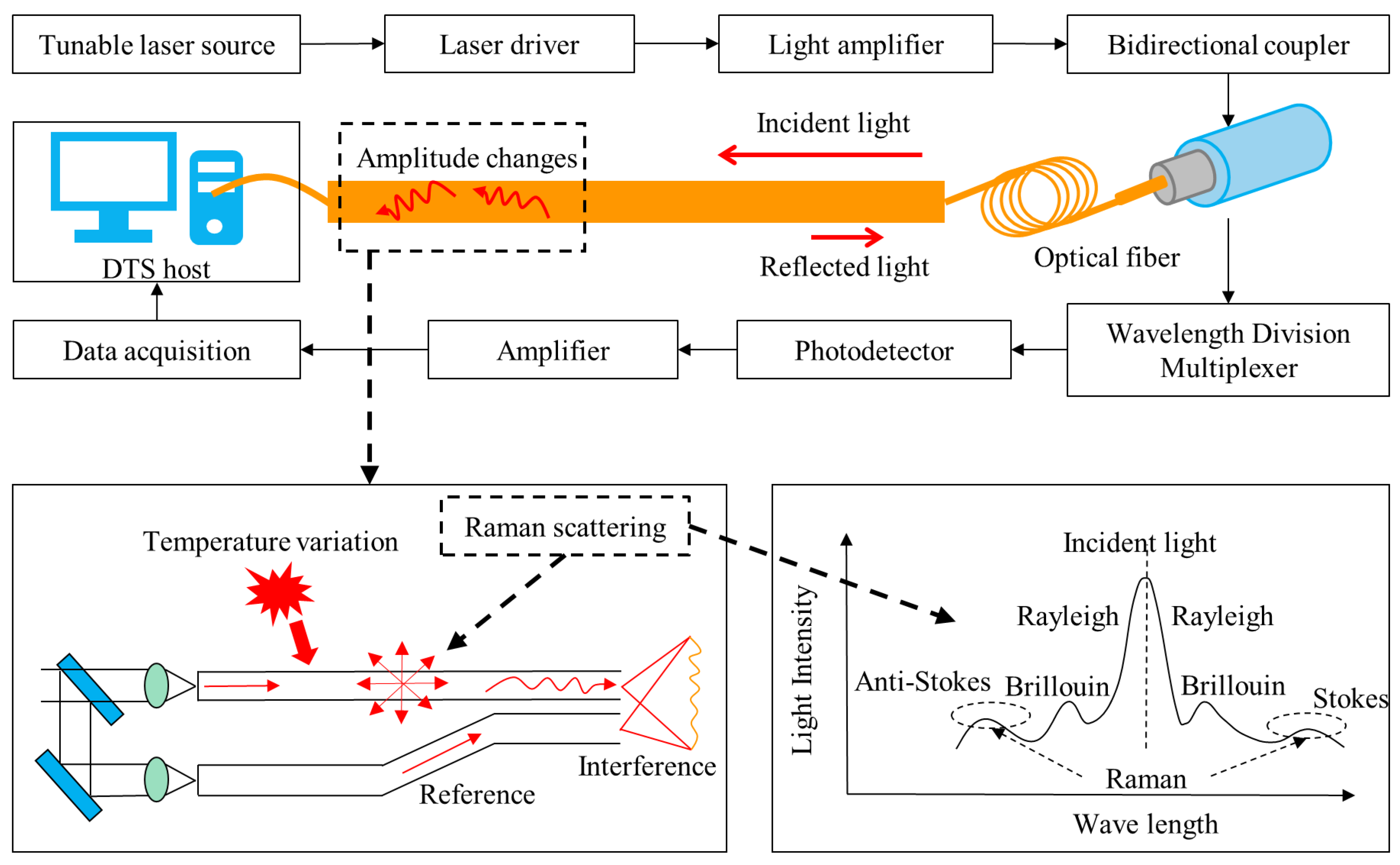
2.1. Distributed Temperature Sensing (DTS)
- Principle of Temperature Measurement
- 2.
- Components of the DTS System
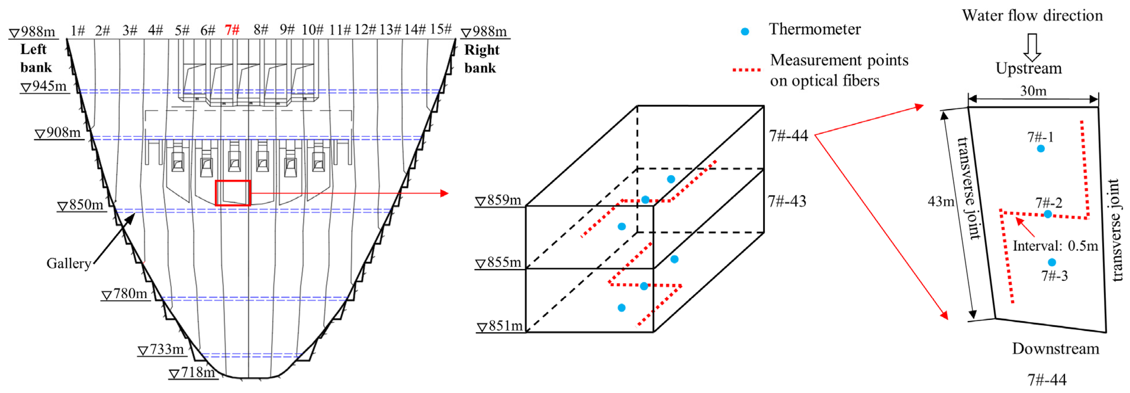
2.2. DTS System Layout and Data Acquisition
3. Optimization Method for Thermal Field Reconstruction
3.1. Interpolation Algorithm Evaluation and Selection
3.1.1. Interpolation Algorithm Comparison
- Kriging
- 2.
- Natural Neighbor
- 3.
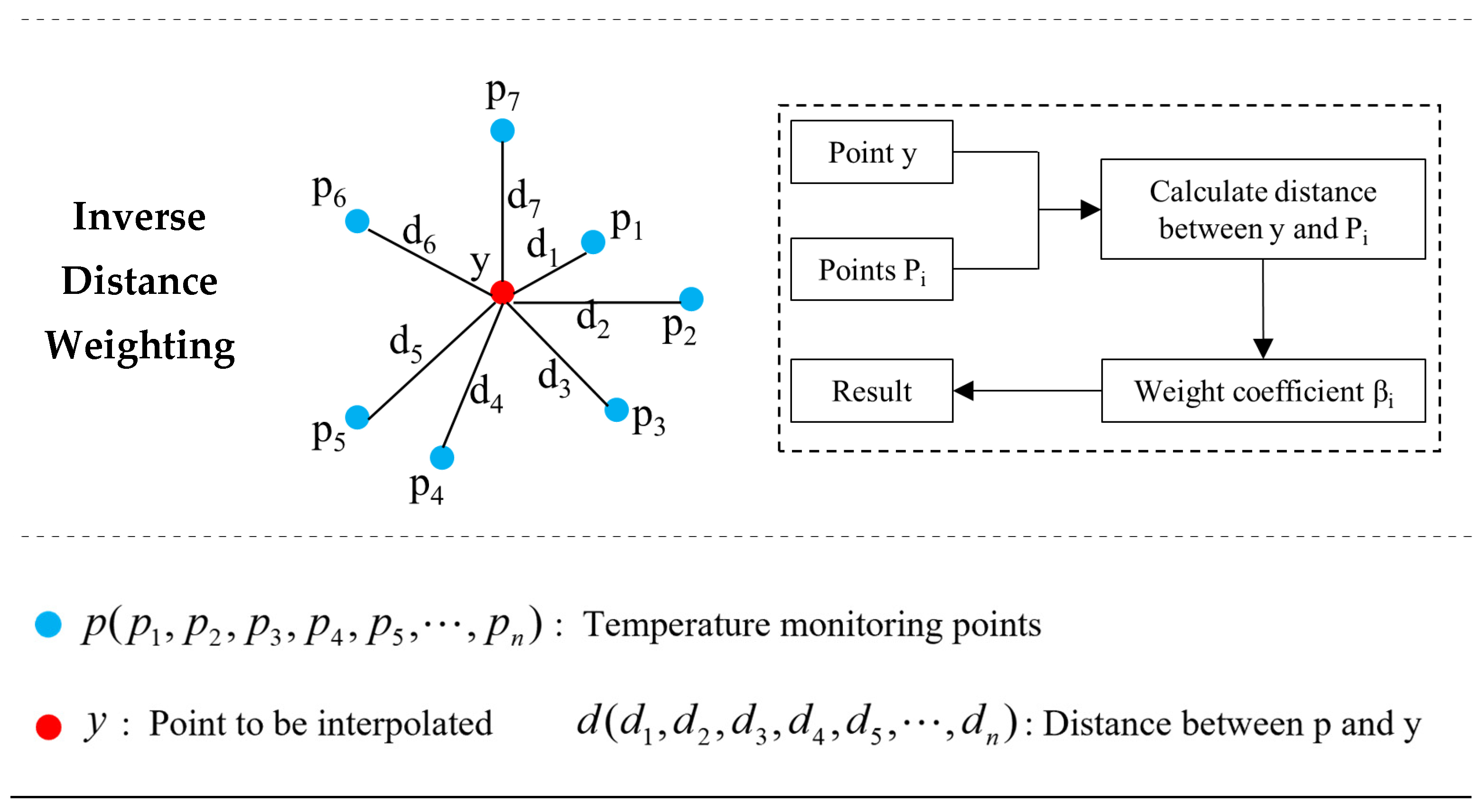
- Inverse Distance Weighting
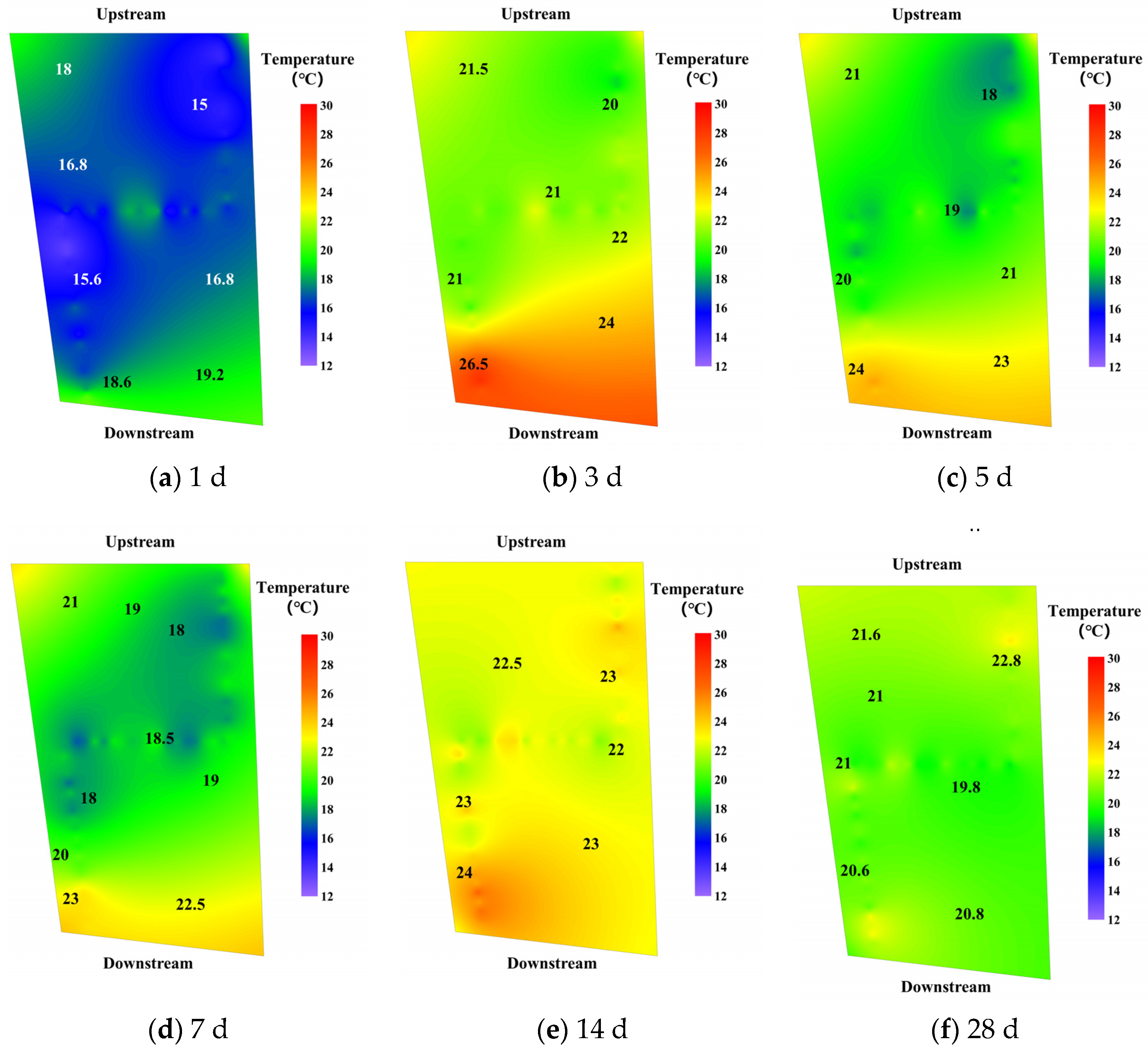
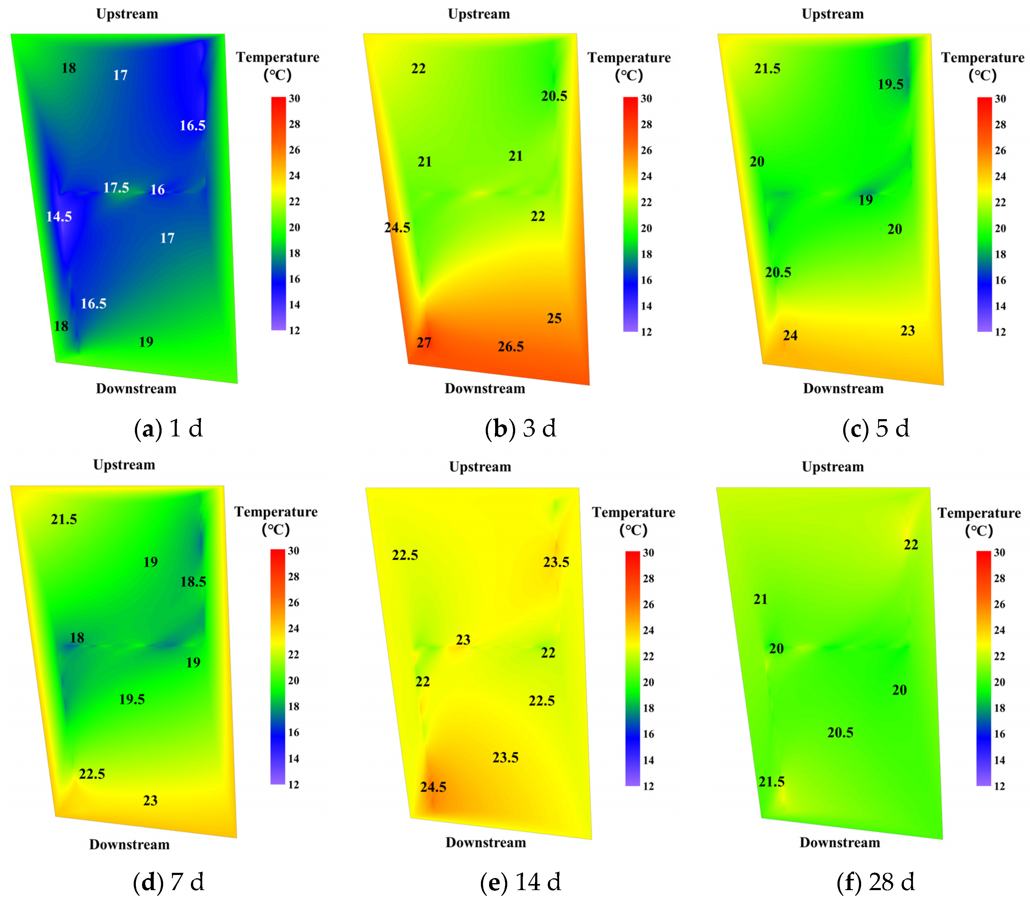
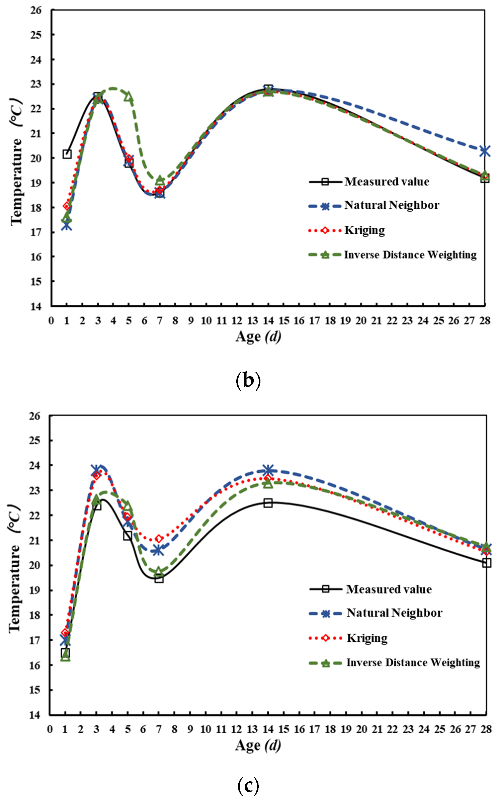
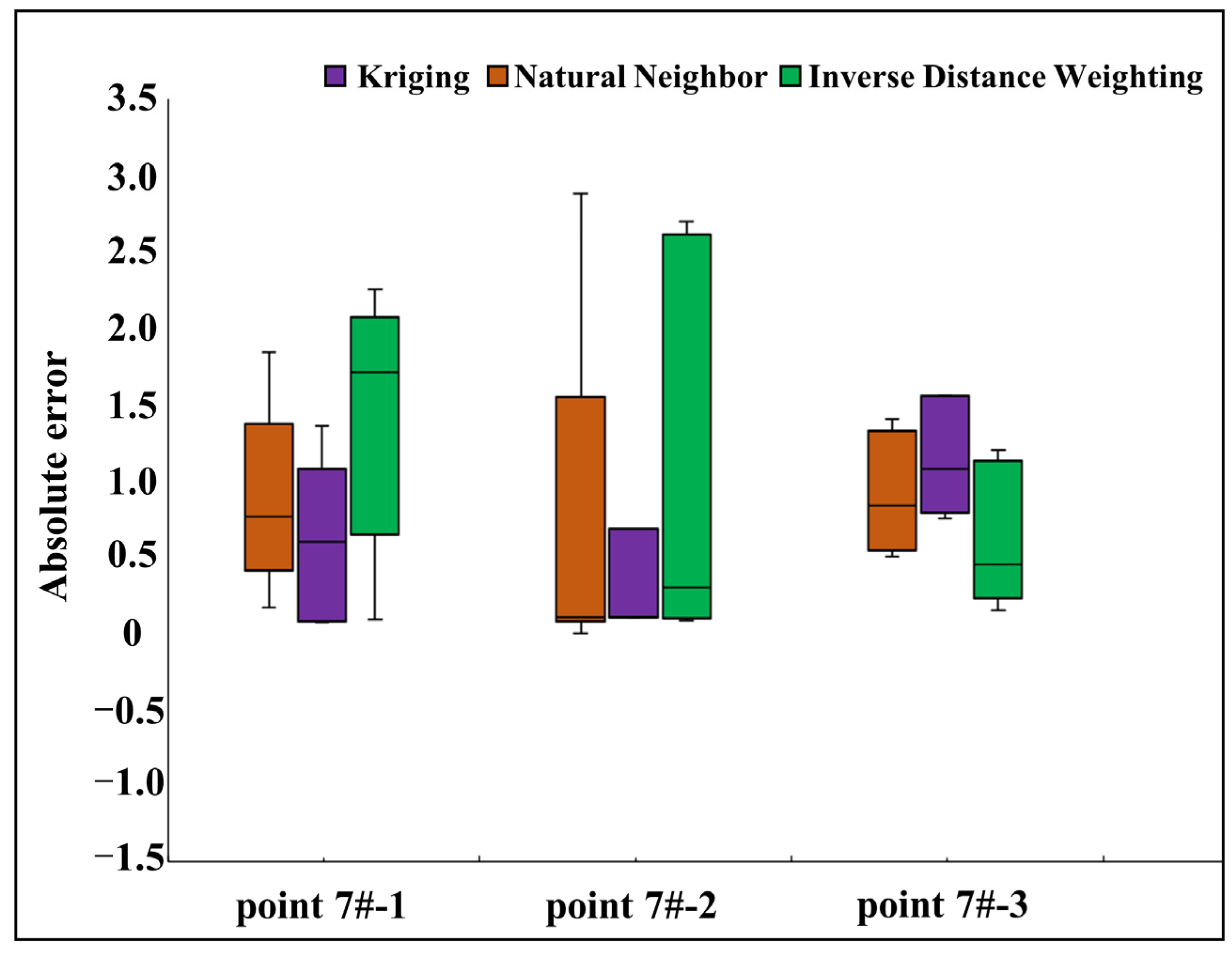
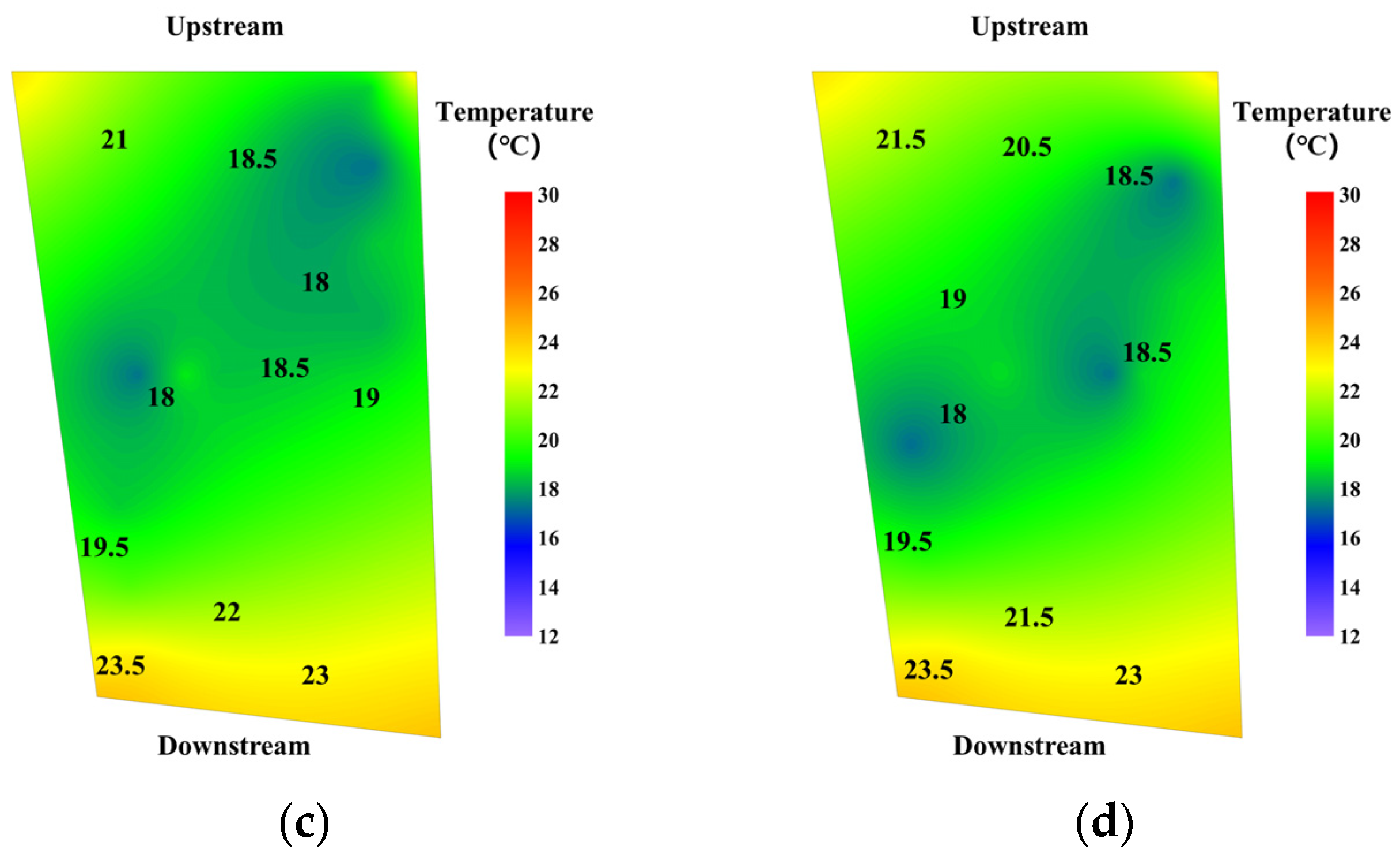
3.1.2. Evaluation of Thermal Field Reconstruction Effectiveness
- Kriging
- 2.
- Natural Neighbor
- 3.
- Inverse Distance Weighting
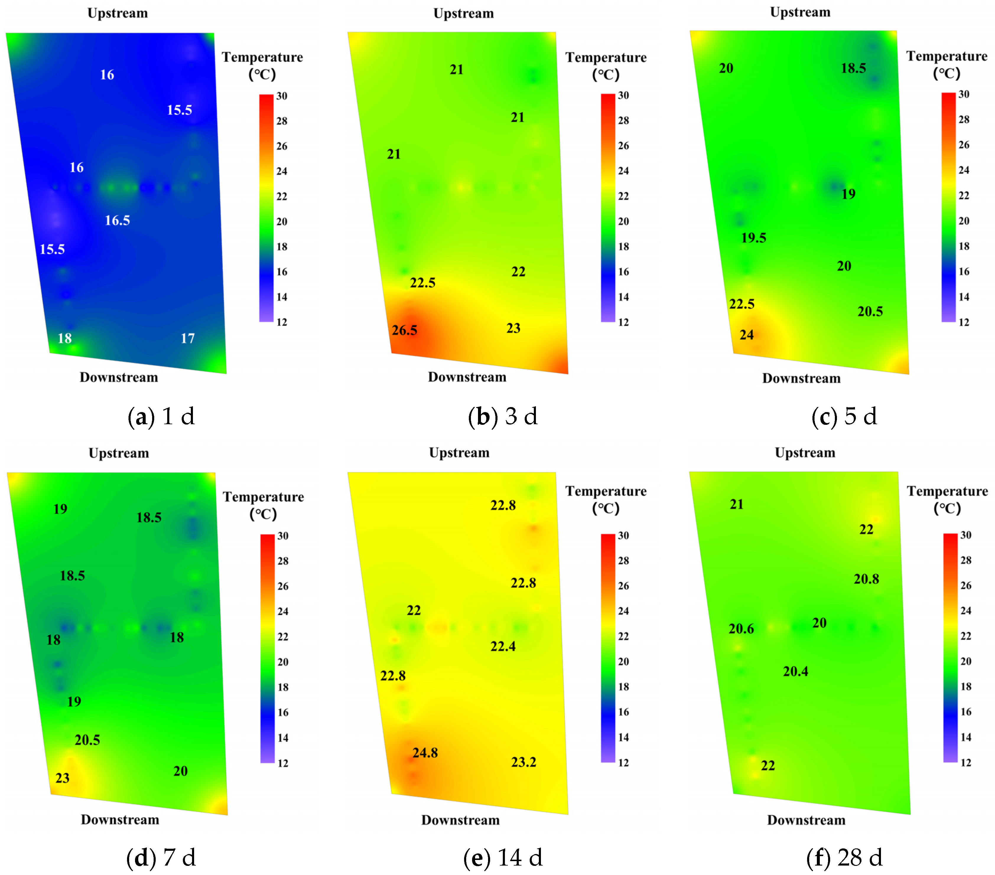
3.1.3. Interpolation Algorithm Selection
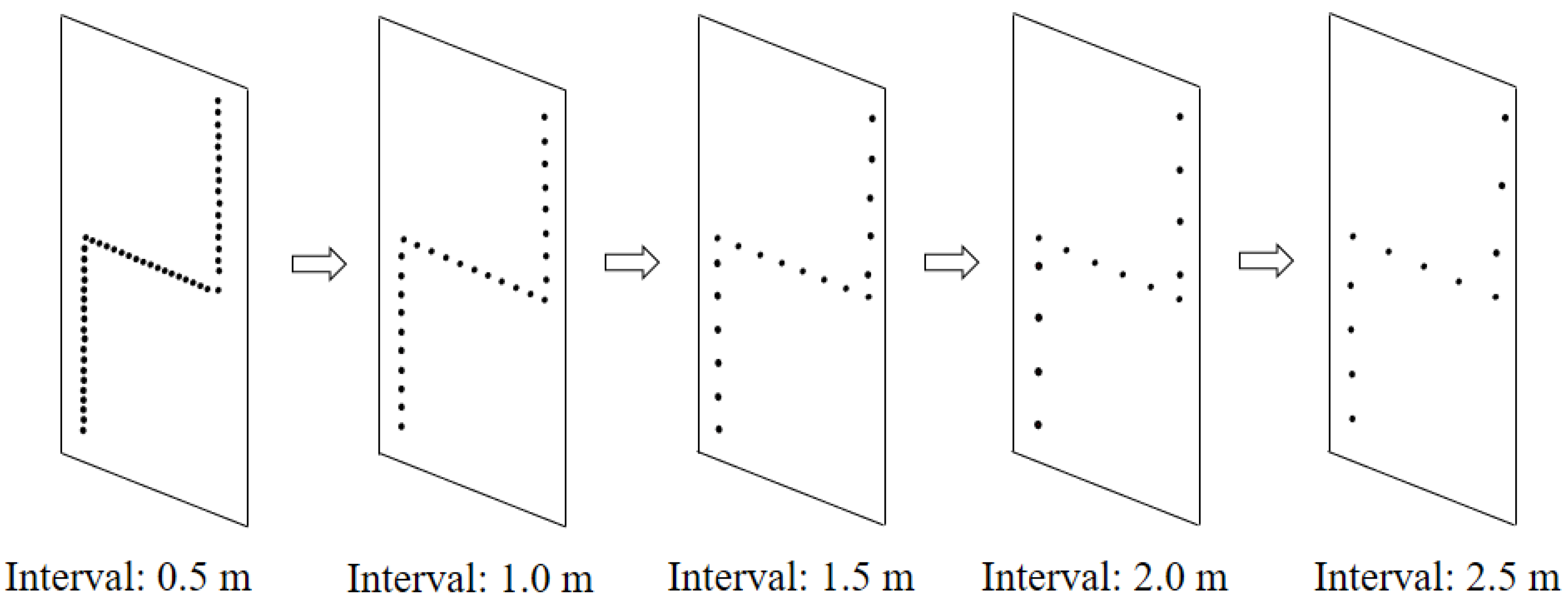
3.2. Monitoring Point Number Optimization
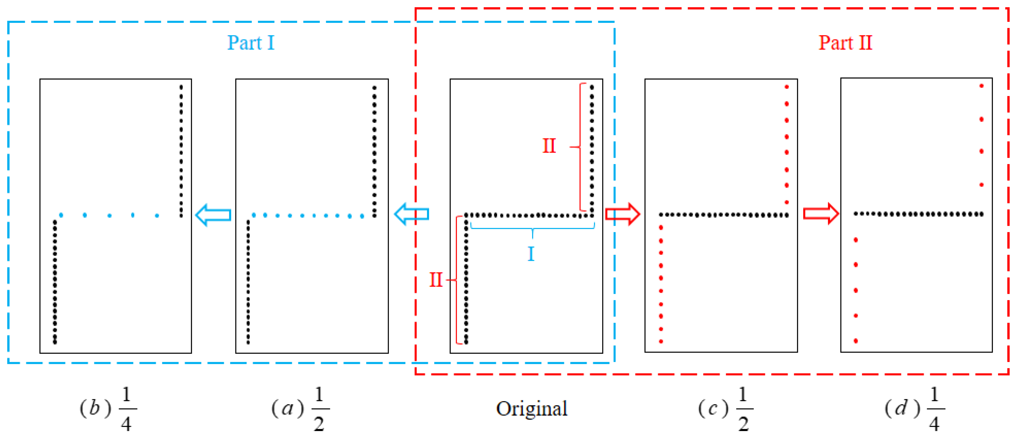
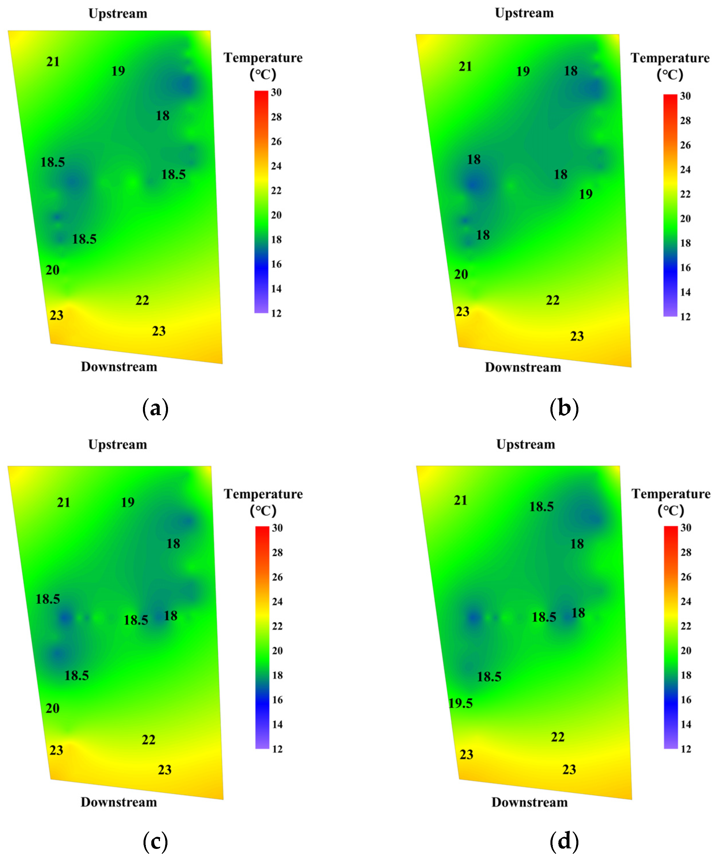
3.3. Analysis of the Impact of Monitoring Positions
- Part I
- 2.
- Part II
3.4. Lightweight Application Procedures
- Monitoring system layout and interpolation algorithm selection
- 2.
- Optimization of thermal field reconstruction Efficiency
- 3.
- Development and implementation of temperature control measures
- 4.
- Evaluation of temperature control effectiveness
4. Case Study
4.1. Project Overview
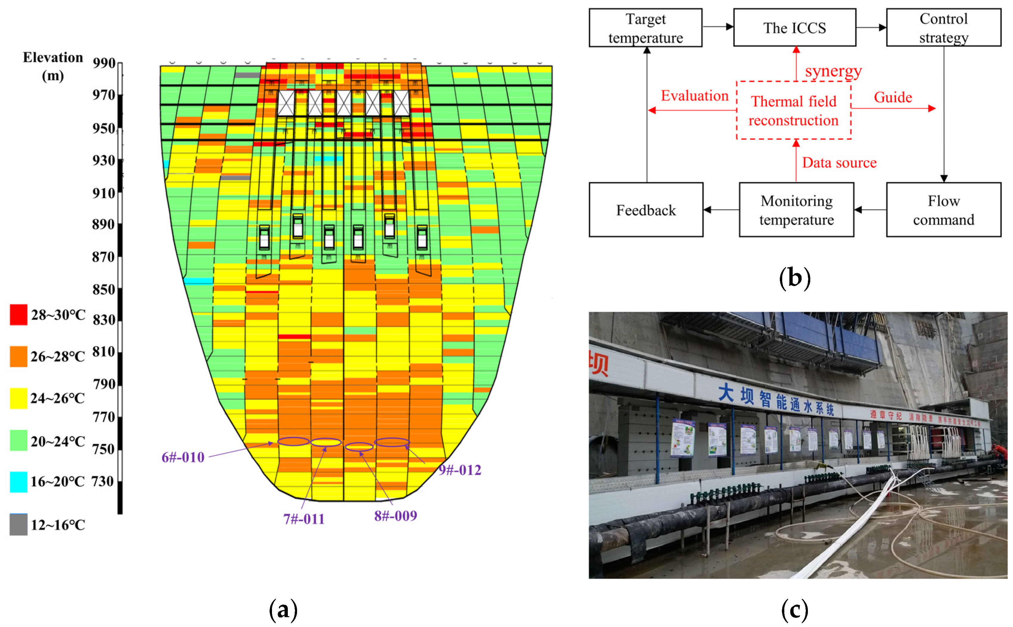
4.2. Effectiveness Evaluation
5. Conclusions
- (1)
- An optimization method for improving the efficiency of thermal field reconstruction was proposed. The applicability of Kriging, Natural Neighbor, and Inverse Distance Weighting interpolation algorithms is evaluated quantitatively based on the actual optical fiber layout scheme. The Kriging is the optimal one when the optical fiber is embedded in a “Z shape”. The reconstructed thermal field was in accordance with the point measurements by digital thermometers, and the mean absolute error and root mean squared error were 0.75 and 0.96, respectively.
- (2)
- The impact of the number and position of monitoring points on thermal field reconstruction was analyzed. Sensitivity analysis indicated that with a “Z-shaped” optical fiber and the Kriging interpolation algorithm, reducing the number of temperature-monitoring points lowers calculation complexity and improves response speed while maintaining accuracy (error < 1 °C). Monitoring points near the transverse joint had a greater effect on reconstruction accuracy than those at the center of the concrete block.
- (3)
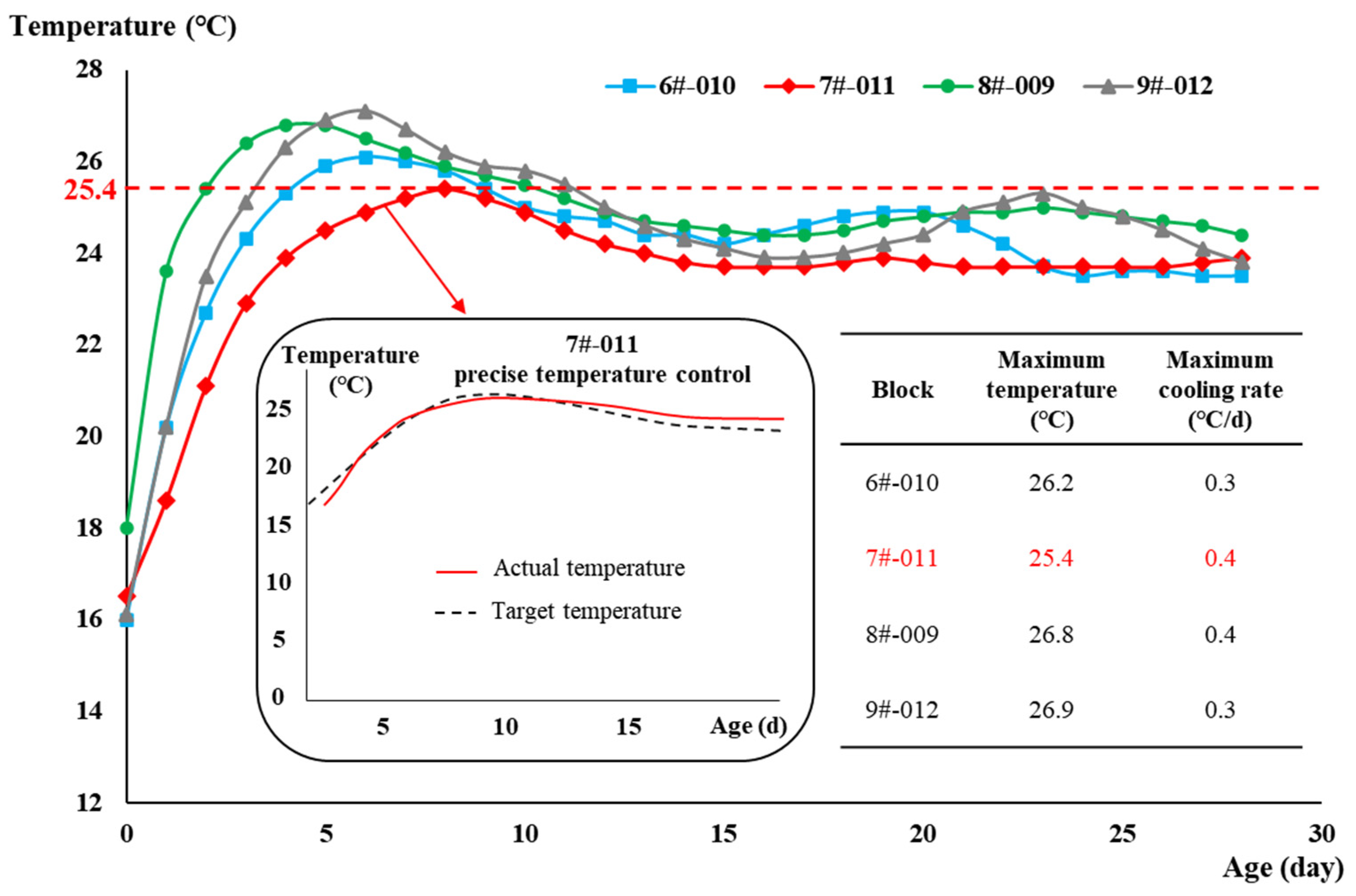
- The method was combined with the intelligent cooling control system, and the effectiveness was verified in the 7# dam monolith of the WDD dam. The maximum temperature of the concrete block is 25.4 °C (meeting the requirement of not exceeding 27 °C). Compared with the dam monolith without this method, the 7# dam monolith has a smoother temperature curve and a cooling rate of 0.4 °C/day (meeting the requirement of 0.3–0.5 °C/day).
Author Contributions
Funding
Institutional Review Board Statement
Informed Consent Statement
Data Availability Statement
Conflicts of Interest
References
- Peng, H.; Lin, P.; Xiang, Y.; Hu, J.; Yang, Z. Effects of carbon thin film on low-heat cement hydration, temperature and strength of the wudongde dam concrete. Buildings 2022, 12, 717. [Google Scholar] [CrossRef]
- Wang, L.; Yang, H.; Zhou, S.; Chen, E.; Tang, S.W. Mechanical properties, long-term hydration heat, shinkage behavior and crack resistance of dam concrete designed with low heat Portland (LHP) cement and fly ash. Constr. Build. Mater. 2018, 187, 1073–1091. [Google Scholar] [CrossRef]
- Xu, D.; Tang, J.; Hu, X.; Yu, C.; Han, F.; Sun, S.; Deng, W.; Liu, J. The influence of curing regimes on hydration, microstructure and compressive strength of ultra-high performance concrete: A review. J. Build. Eng. 2023, 76, 107401. [Google Scholar] [CrossRef]
- Pang, X.; Sun, L.; Chen, M.; Xian, M.; Cheng, G.; Liu, Y.; Qin, J. Influence of curing temperature on the hydration and strength devel-opment of Class G Portland cement. Cem. Concr. Res. 2022, 156, 106776. [Google Scholar] [CrossRef]
- Lin, P.; Ning, Z.; Shi, J.; Liu, C.; Chen, W.; Tan, Y. Study on the gallery structure cracking mechanisms and cracking control in dam construction site. Eng. Fail. Anal. 2021, 121, 105135. [Google Scholar] [CrossRef]
- Ning, Z.; Lin, P.; Ouyang, J.; Yang, Z.; He, M.; Ma, F. Intelligent cooling control for mass concrete relating to spiral case structure. Adv. Concr. Constr. 2022, 14, 57–70. [Google Scholar]
- Žvanut, P.; Turk, G.; Kryžanowski, A. Thermal analysis of a concrete dam taking into account insolation, shading, water level and spillover. Appl. Sci. 2021, 11, 705. [Google Scholar] [CrossRef]
- Li, M.; Lin, P.; Chen, D.; Li, Z.; Liu, K.; Tan, Y. An ANN-based short-term temperature forecast model for mass concrete cooling control. Tsinghua Sci. Technol. 2022, 28, 511–524. [Google Scholar] [CrossRef]
- Groz, M.-M.; Bensalem, M.; Sommier, A.; Abisset-Chavanne, E.; Chevalier, S.; Chulkov, A.; Battaglia, J.-L.; Batsale, J.-C.; Pradere, C. Estimation of thermal resistance field in layered materials by analytical asymptotic method. Appl. Sci. 2020, 10, 2351. [Google Scholar] [CrossRef]
- Zhou, H.; Tian, X.; Wu, J. Cracking and thermal resistance in concrete: Coupled thermo-mechanics and phase-field modeling. Theor. Appl. Fract. Mech. 2024, 130, 104285. [Google Scholar] [CrossRef]
- Klemczak, B.; Smolana, A.; Jędrzejewska, A. Modeling of Heat and Mass Transfer in Cement-Based Materials during Cement Hydration—A Review. Energies 2024, 17, 2513. [Google Scholar] [CrossRef]
- Häfner, S.; Eckardt, S.; Luther, T.; Könke, C. Mesoscale modeling of concrete: Geometry and numerics. Comput. Struct. 2006, 84, 450–461. [Google Scholar] [CrossRef]
- Afzal, J.; Yihong, Z.; Aslam, M.; Qayum, M. A study on thermal analysis of under-construction concrete dam. Case Stud. Constr. Mater. 2022, 17, e01206. [Google Scholar] [CrossRef]
- Mirković, U.; Kuzmanović, V.; Todorović, G. Long-Term Thermal Stress Analysis and Optimization of Contraction Joint Distance of Concrete Gravity Dams. Appl. Sci. 2022, 12, 8163. [Google Scholar] [CrossRef]
- Zhou, Y.; Liang, C.; Wang, F.; Zhao, C.; Zhang, A.; Tan, T.; Gong, P. Field test and numerical simulation of the thermal insulation effect of concrete pouring block surface based on DTS. Constr. Build. Mater. 2022, 343, 128022. [Google Scholar] [CrossRef]
- Wang, F.; Zhao, C.; Zhou, Y.; Zhou, H.; Liang, Z.; Wang, F.; Seman, E.A.; Zheng, A. Multiple Thermal Parameter Inversion for Concrete Dams Using an Integrated Surrogate Model. Appl. Sci. 2023, 13, 5407. [Google Scholar] [CrossRef]
- Hu, J.; Li, K.; Wu, Y.; Zeng, D.; Wang, Z. Optimization of the Cooling Scheme of Artificial Ground Freezing Based on Finite Element Analysis: A Case Study. Appl. Sci. 2022, 12, 8618. [Google Scholar] [CrossRef]
- Chen, M.; Liu, S.; Sun, S.; Liu, Z.; Zhao, Y. Rapid reconstruction of simulated and experimental temperature fields based on proper orthogonal decomposition. Appl. Sci. 2020, 10, 3729. [Google Scholar] [CrossRef]
- Zhou, H.; Pan, Z.; Liang, Z.; Zhao, C.; Zhou, Y.; Wang, F. Temperature field reconstruction of concrete dams based on distributed optical fiber monitoring data. KSCE J. Civ. Eng. 2019, 23, 1911–1922. [Google Scholar] [CrossRef]
- Guo, Y.; Wang, K.; Leng, G.; Zhao, F.; Bao, H. Real-time temperature field reconstruction using a few measurement points and RPIM-AGQ6 interpolation. Measurement 2024, 225, 114041. [Google Scholar] [CrossRef]
- Liu, J.; Wang, F.; Jiang, X.; Mao, D.; Wang, X. Optimization of distributed optical fiber temperature monitoring points based on 3D temperature field reconstruction. Therm. Sci. Eng. Prog. 2024, 53, 102741. [Google Scholar] [CrossRef]
- Lin, P.; Peng, H.; Fan, Q.; Xiang, Y.; Yang, Z.; Yang, N. A 3D thermal field restructuring method for concrete dams based on real-time temperature monitoring. KSCE J. Civ. Eng. 2021, 25, 1326–1340. [Google Scholar] [CrossRef]
- Zhou, H.; Zhou, Y.; Zhao, C.; Wang, F.; Liang, Z. Feedback design of temperature control measures for concrete dams based on real-time temperature monitoring and construction process simulation. KSCE J. Civ. Eng. 2018, 22, 1584–1592. [Google Scholar] [CrossRef]
- Peng, H.; Lin, P.; Xiang, Y.; Chen, W.; Zhou, S.; Yang, N.; Qiao, Y. A positioning method of temperature sensors for monitoring dam global thermal field. Front. Mater. 2020, 7, 587738. [Google Scholar] [CrossRef]
- Zhou, H.; Zhao, C.; Liang, Z.; Zhou, Y.; Wang, F. Method and Application of Spatial Positioning for Valid Temperature-measuring Optical Fibers in Concrete Dams. KSCE J. Civ. Eng. 2023, 27, 3484–3500. [Google Scholar] [CrossRef]
- Yu, H.; Wang, F.; Mao, D.; Chen, J.; Xiong, X.; Song, R.; Liu, J. Temperature monitoring and simulation analysis of the bottom orifices of Baihetan arch dam when outflowing. Int. Commun. Heat Mass Transf. 2024, 150, 107200. [Google Scholar] [CrossRef]
- Imanian, H.; Shirkhani, H.; Mohammadian, A.; Cobo, J.H.; Payeur, P. Spatial interpolation of soil temperature and water content in the land-water interface using artificial intelligence. Water 2023, 15, 473. [Google Scholar] [CrossRef]
- Iversen, S.C.; Sperrevik, A.K.; Goux, O. Improving sea surface temperature in a regional ocean model through refined sea surface temperature assimilation. Ocean Sci. 2023, 19, 729–744. [Google Scholar] [CrossRef]
- Hassani, A.; Santos, G.S.; Schneider, P.; Castell, N. Interpolation, satellite-based machine learning, or meteorological simulation? A comparison analysis for spatio-temporal mapping of mesoscale urban air temperature. Environ. Model. Assess. 2024, 29, 291–306. [Google Scholar] [CrossRef]
- Chen, Z.; Zheng, D.; Li, J.; Wu, X.; Qiu, J. Temperature Field Online Reconstruction for In-Service Concrete Arch Dam Based on Limited Temperature Observation Data Using AdaBoost-ANN Algorithm. Math. Probl. Eng. 2021, 2021, 9979994. [Google Scholar] [CrossRef]
- Li, H.-J.; Zhu, H.-H.; Tan, D.-Y.; Shi, B.; Yin, J.-H. Detecting pipeline leakage using active distributed temperature Sensing: Theoretical modeling and experimental verification. Tunn. Undergr. Space Technol. 2023, 135, 105065. [Google Scholar] [CrossRef]
- Meng, X.; Wang, S.; Fang, N.; Wang, L. Distributed optical fiber sensing system based on semiconductor lasers with mutual un-balanced double optical injection. Optik 2023, 278, 170706. [Google Scholar] [CrossRef]
- Zhang, Z.; Tian, Z.; Wu, Z.; Xu, B. Development and analysis of a BP-LSTM-Kriging temperature field prediction model for the arch ring section of the reinforced concrete arch bridge. Structures 2024, 64, 106564. [Google Scholar] [CrossRef]
- Musashi, J.P.; Pramoedyo, H.; Fitriani, R. Comparison of inverse distance weighted and natural neighbor interpolation method at air temperature data in Malang region. CAUCHY J. Mat. Murni Dan Apl. 2018, 5, 48–54. [Google Scholar] [CrossRef]
- Tan, J.; Xie, X.; Zuo, J.; Xing, X.; Liu, B.; Xia, Q.; Zhang, Y. Coupling random forest and inverse distance weighting to generate climate surfaces of precipitation and temperature with Multiple-Covariates. J. Hydrol. 2021, 598, 126270. [Google Scholar] [CrossRef]
- Amira, Z.; Bouyahi, M.; Ezzedine, T. Measurement of Temperature through Raman Scattering. Procedia Comput. Sci. 2015, 73, 350–357. [Google Scholar] [CrossRef]
- Pei, H.-F.; Teng, J.; Yin, J.-H.; Chen, R. A review of previous studies on the applications of optical fiber sensors in geotechnical health monitoring. Measurement 2014, 58, 207–214. [Google Scholar] [CrossRef]
- Ma, Y.; Zhang, Y.; Cheng, Y.; Zhang, Y.; Gao, X.; Shan, K. A case study of field thermal response test and laboratory test based on distributed optical fiber temperature sensor. Energies 2022, 15, 8101. [Google Scholar] [CrossRef]
- Palmieri, L.; Schenato, L. Distributed optical fiber sensing based on Rayleigh scattering. Open Opt. J. 2013, 7, 104–127. [Google Scholar] [CrossRef]
- Muanenda, Y.; Oton, C.J.; Di Pasquale, F. Application of Raman and Brillouin scattering phenomena in distributed optical fiber sensing. Front. Phys. 2019, 7, 155. [Google Scholar] [CrossRef]
- Ouyang, J.; Chen, X.; Huangfu, Z.; Lu, C.; Huang, D.; Li, Y. Application of distributed temperature sensing for cracking control of mass concrete. Constr. Build. Mater. 2019, 197, 778–791. [Google Scholar] [CrossRef]
- Su, H.; Cui, S.; Wen, Z.; Xie, W. Experimental study on distributed optical fiber heated-based seepage behavior identification in hydraulic engineering. Heat Mass Transf. 2019, 55, 421–432. [Google Scholar] [CrossRef]
- Zhao, D.; Wang, Y.; Liang, D. Correlating variations in the dynamic power signature to nugget diameter in resistance spot welding using Kriging model. Measurement 2019, 135, 6–12. [Google Scholar] [CrossRef]
- Rodrigues, D.; Belinha, J.; Dinis, L.; Jorge, R.N. The numerical analysis of symmetric cross-ply laminates using the natural neighbour radial point interpolation method and high-order shear deformation theories. Eng. Struct. 2020, 225, 111247. [Google Scholar] [CrossRef]
- Dogan, T.; Kastner, P.; Mermelstein, R. Surfer: A fast simulation algorithm to predict surface temperatures and mean radiant temperatures in large urban models. Build. Environ. 2021, 196, 107762. [Google Scholar] [CrossRef]
- Protasov, A. Reconstruction of the thermal field image from measurements in separate points. In Proceedings of the 2017 IEEE Microwaves, Radar and Remote Sensing Symposium (MRRS), Kiev, Ukraine, 29–31 August 2017; IEEE: Piscataway, NJ, USA, 2017; pp. 89–92. [Google Scholar]
- Billo, G.; Belliard, M.; Sagaut, P. Comparison of several interpolation methods to reconstruct field data in the vicinity of a finite element immersed boundary. Comput. Math. Appl. 2022, 123, 123–135. [Google Scholar] [CrossRef]
- Zhao, X.; Chen, X.; Gong, Z.; Zhou, W.; Yao, W.; Zhang, Y. RecFNO: A resolution-invariant flow and heat field reconstruction method from sparse observations via Fourier neural operator. Int. J. Therm. Sci. 2024, 195, 108619. [Google Scholar] [CrossRef]


| Interpolation Algorithm | Position | Minimum Error (°C) | Maximum Error (°C) | Average Error (°C) |
|---|---|---|---|---|
| Kriging | 7#-1 | 0.07 | 1.36 | 0.76 |
| 7#-2 | 0.10 | 2.13 | ||
| 7#-3 | 0.75 | 1.55 | ||
| Natural Neighbor | 7#-1 | 0.17 | 1.84 | 0.81 |
| 7#-2 | 0.00 | 2.88 | ||
| 7#-3 | 0.50 | 1.40 | ||
| Inverse Distance Weighting | 7#-1 | 0.09 | 2.25 | 0.96 |
| 7#-2 | 0.08 | 2.58 | ||
| 7#-3 | 0.15 | 1.20 |
| Interpolation Algorithm | Position | MAE | RMSE | Average MAE | Average RMSE |
|---|---|---|---|---|---|
| Kriging | 7#-1 | 0.68 | 0.84 | 0.75 | 0.96 |
| 7#-2 | 0.46 | 0.88 | |||
| 7#-3 | 1.11 | 1.15 | |||
| Natural Neighbor | 7#-1 | 0.83 | 0.97 | 0.82 | 1.07 |
| 7#-2 | 0.71 | 1.26 | |||
| 7#-3 | 0.90 | 0.98 | |||
| Inverse Distance Weighting | 7#-1 | 1.26 | 1.48 | 0.96 | 1.25 |
| 7#-2 | 1.01 | 1.54 | |||
| 7#-3 | 0.60 | 0.73 |
Disclaimer/Publisher’s Note: The statements, opinions and data contained in all publications are solely those of the individual author(s) and contributor(s) and not of MDPI and/or the editor(s). MDPI and/or the editor(s) disclaim responsibility for any injury to people or property resulting from any ideas, methods, instructions or products referred to in the content. |
© 2024 by the authors. Licensee MDPI, Basel, Switzerland. This article is an open access article distributed under the terms and conditions of the Creative Commons Attribution (CC BY) license (https://creativecommons.org/licenses/by/4.0/).
Share and Cite
Xiang, Y.; Lin, P.; Peng, H.; Li, Z.; Liu, Y.; Qiao, Y.; Yang, Z. Optimization Method for Improving Efficiency of Thermal Field Reconstruction in Concrete Dam. Appl. Sci. 2024, 14, 10857. https://doi.org/10.3390/app142310857
Xiang Y, Lin P, Peng H, Li Z, Liu Y, Qiao Y, Yang Z. Optimization Method for Improving Efficiency of Thermal Field Reconstruction in Concrete Dam. Applied Sciences. 2024; 14(23):10857. https://doi.org/10.3390/app142310857
Chicago/Turabian StyleXiang, Yunfei, Peng Lin, Haoyang Peng, Zichang Li, Yuanguang Liu, Yu Qiao, and Zuobin Yang. 2024. "Optimization Method for Improving Efficiency of Thermal Field Reconstruction in Concrete Dam" Applied Sciences 14, no. 23: 10857. https://doi.org/10.3390/app142310857
APA StyleXiang, Y., Lin, P., Peng, H., Li, Z., Liu, Y., Qiao, Y., & Yang, Z. (2024). Optimization Method for Improving Efficiency of Thermal Field Reconstruction in Concrete Dam. Applied Sciences, 14(23), 10857. https://doi.org/10.3390/app142310857