Vehicle Motion Control for Overactuated Vehicles to Enhance Controllability and Path Tracking

Featured Application

To explore the benefits of an overactuated vehicle at the limits of handling for autonomous driving. Development of a layered, modular, and computationally efficient control architecture for vehicles equipped with wheel-independent motors and axle-wise independent steering by separating the actuator allocation from the path tracking task.

Abstract

The motion control of vehicles poses distinct challenges for both vehicle stability and path tracking, especially under critical environmental and driving conditions. Overactuated vehicles can effectively utilize the available tyre–road friction potential by leveraging additional actuators, thus enhancing their stability and controllability even in challenging scenarios. This paper introduces a novel modular upstream control architecture for overactuated vehicles, integrating a fast and robust linear time-varying model predictive path and speed tracking controller with a model following approach and nonlinear control allocation to form a holistic vehicle motion controller. The architecture decouples the path and speed tracking task from the actuator allocation, where torque vectoring and rear-wheel steering are applied to achieve linear understeer reference vehicle behavior. It allows for the use of a simpler path tracking controller, enabling long preview horizons and enhanced computational efficiency. Nonlinearities, such as the mutual influence of lateral and longitudinal tyre forces, are accounted for within the control allocation. The simulation results demonstrate that the proposed control architecture and overactuation improve vehicle stability in critical driving conditions and reduce path tracking errors compared to a dual-motor vehicle.

1. Introduction

With the electrification of powertrains, the number of drive motors in vehicles is increasing. Vehicle configurations are evolving from dual-motors for all-wheel drive to tri-motor systems with rear-axle torque vectoring (TV) and potentially to four motors [1]. Additionally, active front- and rear-wheel steering systems are being integrated to support automated driving functions. This raises the question of the advantages provided by multiple actuators for autonomous driving. Specifically, how do four-wheel steering (4WS) and wheel-independent four-wheel drive (4WD) influence vehicle handling, path tracking, and the stable domain of vehicle motion?

A diversified set of actuators, as highlighted by [2] in Figure 1, allows integrated control or global chassis control to make optimal use of the available tyre–road friction potential [3,4]. These integrated control strategies are part of the vehicle motion controller (VMC) in Figure 2, which facilitates the matched use of the available chassis actuators [5,6]. By decoupling individual wheels with electric motors, TV can effectively be used to shape the vehicle response and influence its stability [7,8,9]. Improved vehicle performance benefits both manual and automated driving.

Early path tracking controllers, such as pure pursuit controllers [10], operate without inherent vehicle stability considerations and heavily rely on electronic stability control (ESC). Advances in control theory, particularly model predictive control (MPC), integrate stability considerations through nonlinear vehicle models [11], stability constraints with a stability envelope (SE) based on phase plane analysis [12,13,14,15], or positive invariant sets to constrain MPC within a robust tube [16].

In [17], the stable handling envelope is further extended by effectively using 4WS and TV. Despite relying on a linear tyre model and unconstrained control allocation (CA), the method demonstrates a significantly enhanced vehicle response with combined control. Recent advancements, as shown in [18], incorporate nonlinear vehicle models and detailed tyre information. These studies illustrate a TV stability controller based on MPC, which optimizes brake intervention. Meanwhile, Ref. [19] utilizes an optimization-based approach to study the theoretical limits of TV and 4WS for vehicle stability control, highlighting the significant potential for increased vehicle controllability. Ref. [9] demonstrates how TV can be used to adjust the linear understeer characteristics and extend the maximum attainable lateral acceleration by allocating wheel torques through minimum slip-based optimization.

For automated driving, Ref. [20] investigates vehicle stability and minimal lateral displacement during evasive maneuvers by using a basic driver model approach as a controller, combined with a linear CA to optimize tyre force utilization through 4WS and TV. Similarly, Ref. [21] applies offline optimized TV maps with a proportional–integral–derivative (PID) controller to improve the vehicle stability for an autonomous racing vehicle at the limits. However, in both cases, the feedback controllers may exceed the physical limits as the tyre saturations are not considered online. To incorporate detailed tyre information into the feedback controller, Ref. [22] uses a semi-empirical tyre model combined with linear time-varying model predictive control (LTV-MPC) to utilize brakes for TV, improving path tracking.

Despite the vast research on overactuated vehicles for the stabilization and modification of vehicle behavior, there appears to be a research gap regarding the use of overactuated vehicles in automated driving applications and the implications for path and speed tracking controller design, including

• predictable (linear) reference vehicle behavior;
• overactuation to generate the predictable (linear) reference vehicle behavior, as well as to enlarge the stable region for maneuvering at the limits;
• linear and therefore fast MPC, instead of a more complex nonlinear variant, by taking advantage of the (linear) reference vehicle behavior;
• a modular approach that allows switching between different actuator configurations with the same control strategy/architecture;
• a modular approach that allows switching between automated and manual driving without changing the control strategy/architecture.

Addressing these aspects forms the primary focus and novel contribution of this paper.

The remainder of this paper is organized as follows. Section 2 presents the proposed controller architecture. Section 3 introduces the time-varying model predictive path tracking controller. Section 4 and Section 5 first introduce model following (MF), followed by the nonlinear optimal CA. In Section 6, the control architecture is tested for a quasi-steady-state and a transient driving maneuver using a detailed multi-body vehicle model. The vehicle and control properties are analyzed using the phase plane method. Finally, the main outcome of the paper is summarized and conclusions are drawn.

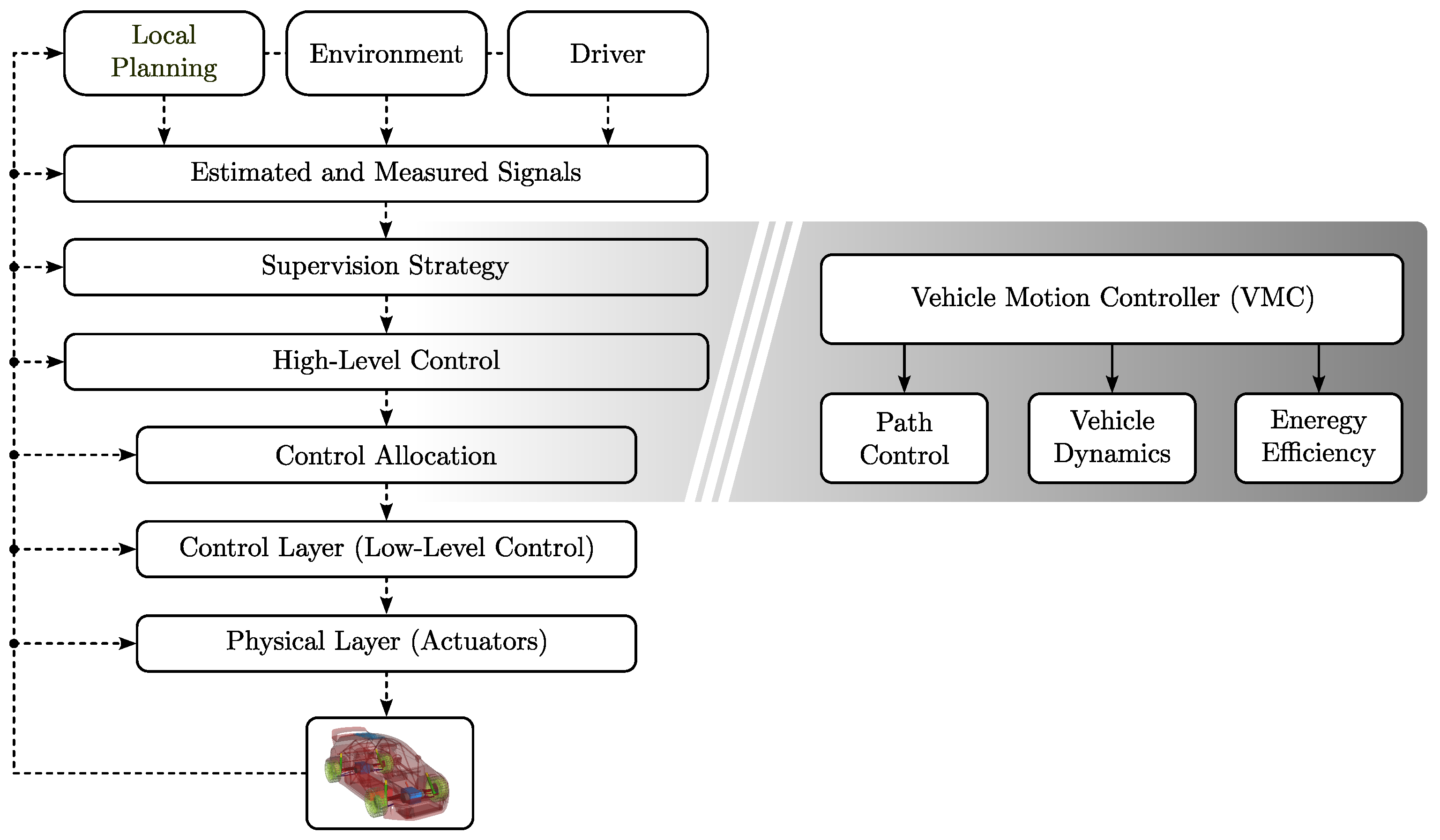
2. Control Architecture

The integrated control of all actuators, while simultaneously tracking a reference path for autonomous path following, can be achieved using a single controller. However, employing a single controller in this manner imposes limitations on the modularity and increases the computational demands [18]. Therefore, in this paper, a modular control architecture is proposed that separates CA from the path tracking task. Additionally, it enables manual vehicle control without modifying the control architecture. However, CA for manual driving is not within the scope of this work. This approach utilizes 4WS and wheel-independent 4WD

• to optimally allocate TV and rear-wheel steering (RWS) to track the (linear) reference vehicle behavior with respect to handling using MF and CA, and
• to utilize this reference vehicle behavior within the MPC framework to create a fast and robust path tracking controller.

The architecture in this paper follows an upstream control approach with layered vehicle control [3,23], as shown in Figure 2. Global demands are refined into actuator commands in lower control layers. Key layers include the supervision strategy, high-level control, and the CA layer. Detailed views of the high-level control and CA are provided in Figure 3.

The control objective is to follow a reference path described by the path length s, curvature $\rho \left(s\right)$ and reference vehicle velocity $V_{\mathrm{ref}}\left(s\right)$ given the current vehicle state, heading error $\theta$ and lateral error e.

The high-level control comprises the LTV-MPC and MF. Unlike nonlinear MPC, this approach results in a convex quadratic program (QP) with linear constraints, allowing for efficient and robust solvers and long prediction horizons in the MPC. Consequently, the high-level control does not account for nonlinearities such as tyre saturations and overactuation. These aspects are accounted for in the CA, which is formulated as a nonlinear optimization problem without preview, being less computationally expensive than MPC.

Both layers are connected through global demands for the longitudinal force ${\overline{\Sigma F}}_x$, lateral force ${\overline{\Sigma F}}_y$ and yaw moment ${\overline{\Sigma M}}_z$ generated by the MF, aiming to align the generated vehicle response with the expected reference vehicle response in the MPC.

Considering the desired linear reference vehicle behavior, a two-wheel vehicle model with linear tyre characteristics is sufficient to design the MPC and MF; see Figure 4a. The planned trajectories of the MPC are constrained within a stability envelope (SE) to address vehicle stability concerns related to tyre staturations [12]. Leveraging the results of [19], which demonstrated the improved controllability of overactuated vehicles with 4WS and TV, and phase plane studies presented in later sections, this work extends the SE limits to accommodate overactuation capabilities. The MPC outputs are the front wheel steering (FWS) speed ${\dot{\delta }}_f$ and drive force $F_d$ to maintain the vehicle velocity given the vehicle state, current path errors $\theta$ and e and a segment of the reference path by ${\mathit{V}}_{\mathrm{ref}}$ and $\rho$ comprising sampled points originating from the current vehicle position and extending until a look-ahead distance; see Figure 3.

In the subsequent CA layer, an optimal CA problem is employed to optimize the tyre force utilization with RWS and TV and trim the vehicle to the desired reference vehicle behavior [24]. Therefore, a four-wheel planar vehicle model is employed for the CA considering the 4WS, tyre load transfer and nonlinear tyre characteristics; see Figure 4b and Section 5. This is intended to make optimal use of the available tyre–road friction potential. The output of the CA includes the RWS angle ${\delta }_r$ and the wheel torques $T_{w,i}$, $i\in \{1,2,3,4\}$, in addition to the feed-through FWS angle ${\delta }_f$. Assuming that the global force and moment demand is achievable by the physical vehicle, the CA algorithm modifies the vehicle dynamics to yield the reference vehicle behavior.

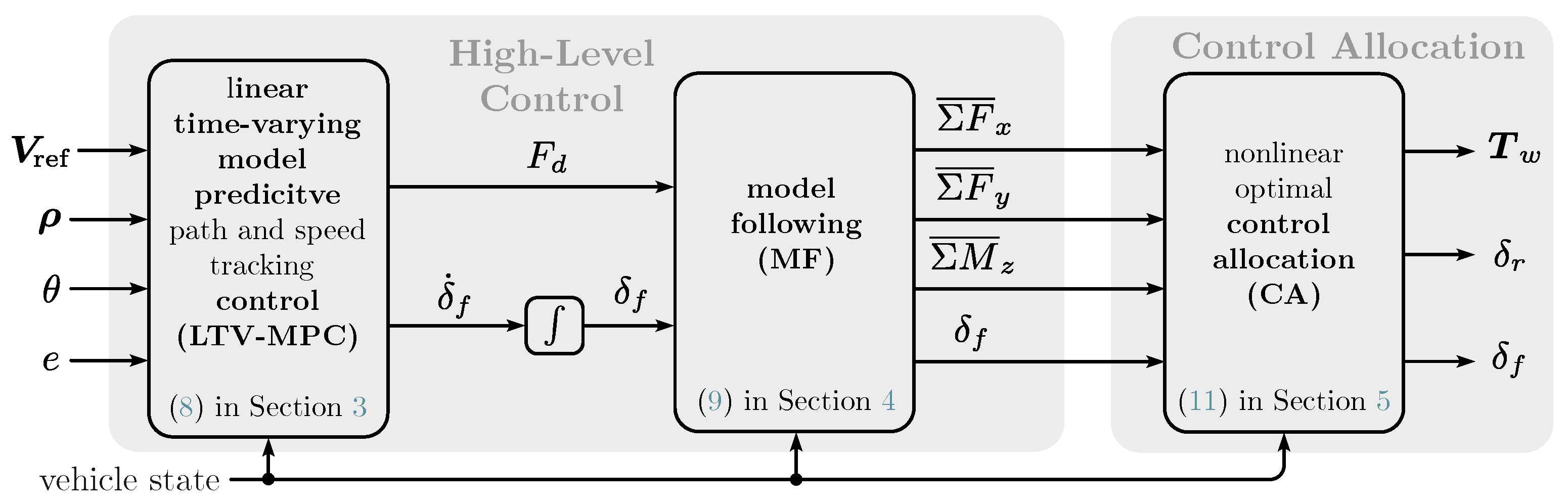
3. Linear Time-Varying Model Predictive Path and Speed Tracking

3.1. Prediction Model

The two-wheel vehicle model depicted in Figure 4a serves as the prediction model for the vehicle’s motion. The longitudinal forces are accounted for by the drive force $F_d$, independently of the lateral forces. The equations of motion (EoM) with the vehicle velocity V, sideslip angle $\beta$ and yaw rate $\dot{\psi }$ read as follows:

$$\begin{array}{cc}\hfill \dot{V}& ={\displaystyle \frac{1}{m}}\left(\Sigma F_{x}cos\beta +\Sigma F_{y}sin\beta \right),\hfill \end{array}$$

(1a)

$$\begin{array}{cc}\hfill \dot{\beta }& ={\displaystyle \frac{1}{Vm}}\left(-\Sigma F_{x}sin\beta +\Sigma F_{y}cos\beta -Vm\dot{\psi }\right),\hfill \end{array}$$

(1b)

$$\begin{array}{cc}\hfill \ddot{\psi }& ={\displaystyle \frac{1}{I_z}}\Sigma M_z,\hfill \end{array}$$

(1c)

with vehicle mass m and yaw moment of inertia $I_z$. $\Sigma F_x$ and $\Sigma F_y$ denote the total forces acting on the vehicle along the respective coordinate frame axes, whereas $\Sigma M_z$ represents the yaw moment generated by the tyres. The total forces and moment yield

$$\begin{array}{cc}\hfill \Sigma F_x& =F_d-F_{y,f}sin{\delta }_f,\hfill \end{array}$$

(2a)

$$\begin{array}{cc}\hfill \Sigma F_y& =F_{y,f}cos{\delta }_f+F_{y,r},\hfill \end{array}$$

(2b)

$$\begin{array}{cc}\hfill \Sigma M_z& =l_f{F}_{y,f}cos{\delta }_f-l_r{F}_{y,r}.\hfill \end{array}$$

(2c)

with the distances $l_f$ and $l_r$ from the center of gravity (CoG) of the vehicle model to the front and rear axle, respectively. The sideslip angles ${\alpha }_f$ and ${\alpha }_r$ of the front and rear axle read

$$\begin{array}{cc}\hfill {\alpha }_f& ={\delta }_f-arctan\left({\displaystyle \frac{l_f\dot{\psi }+Vsin\beta }{Vcos\beta }}\right),\hfill \end{array}$$

(3a)

$$\begin{array}{cc}\hfill {\alpha }_r& =arctan\left({\displaystyle \frac{l_r\dot{\psi }-Vsin\beta }{Vcos\beta }}\right).\hfill \end{array}$$

(3b)

The tyre/axle characteristics of the prediction model may be represented by a nonlinear tyre model, e.g., the tyre brush model [25]. However, considering the assumed linear reference vehicle behavior in this paper, lateral tyre forces are represented by $F_{y,f}=C_f{\alpha }_f$ and $F_{y,r}=C_r{\alpha }_r$, where $C_f$ and $C_r$ denote the respective cornering stiffness.

The motion of the vehicle relative to the reference path is described in a Frenet coordinate system—see Figure 4a—with the lateral error e and the heading error $\theta$ between the longitudinal axis of the vehicle and the tangent to the path with curvature $\rho \left(s\right)$ at length s. The rates of change for the heading error, lateral error and path length are given by [26]

$$\begin{array}{cc}\hfill \dot{\theta }& =\dot{\psi }-\dot{s}\rho \left(s\right)\mathrm{with}\dot{s}={\displaystyle \frac{Vcos\left(\theta +\beta \right)}{1-\rho \left(s\right)e}},\hfill \end{array}$$

(4a)

$$\begin{array}{cc}\hfill \dot{e}& =Vsin\left(\theta +\beta \right).\hfill \end{array}$$

(4b)

The nonlinear, time-continuous system model is obtained from (1) to (4):

$$\dot{\mathit{x}}\left(t\right)={\mathit{f}}_t\left(\mathit{x}\left(t\right),\mathit{u}\left(t\right),\rho \left(s\right)\right)$$

(5)

with the state vector ${\mathit{x}}^T=\left[\begin{array}{cccccc}V& \beta & \dot{\psi }& \theta & e& {\delta }_f\end{array}\right]$ and the input vector ${\mathit{u}}^T=\left[\begin{array}{cc}{\dot{\delta }}_f& F_d\end{array}\right]$. Since the CA may run at a higher sampling rate than the MPC, (5) includes an additional integrator state for ${\delta }_f$ to provide intermediate values for CA via first-order hold.

Since path information, such as the curvature $\rho \left(s\right)$, is available as a function of the path length s, the prediction model is transformed into a space-continuous model. Thus, the system model is rewritten with $\dot{\mathit{x}}=\frac{\partial \mathit{x}}{\partial s}\frac{\partial s}{\partial t}={\mathit{x}}^{\prime }\dot{s}$

$${\mathit{x}}^{\prime }\left(s\right)={\displaystyle \frac{1}{\dot{s}}}{\mathit{f}}_t\left(·\right)={\mathit{f}}_s\left(\mathit{x}\left(s\right),\mathit{u}\left(s\right),\rho \left(s\right)\right),$$

(6)

and linearized by truncating the Taylor series after the first-order term. The discretized linear system equations required for the subsequent optimization problem in the LTV-MPC are derived from the solution of the first-order differential equation system using the zero-order hold assumption,

$$\Delta {\mathit{x}}_{k+1}={\mathit{A}}_{d\left|k\right.}\Delta {\mathit{x}}_k+{\mathit{B}}_{d\left|k\right.}\Delta {\mathit{u}}_k,$$

(7)

with the system matrix ${\mathit{A}}_{d\left|k\right.}$ and the input matrix ${\mathit{B}}_{d\left|k\right.}$. Here, k represents the discrete step index with constant step size $\Delta s$.

3.2. Linear Time-Varying Model Predictive Control (LTV-MPC)

The path tracking controller is formulated as a static, convex optimization problem subject to stability constraints, discrete state space dynamics and actuator constraints:

$$\begin{array}{cccc}& \underset{{\dot{\delta }}_f,{\mathit{F}}_d,{\mathit{s}}_{\dot{\psi }},{\mathit{s}}_{\beta }}{min}\hfill & & \begin{array}{cc}& \stackrel{\mathrm{path}\mathrm{and}\mathrm{speed}\mathrm{tracking}}{\overbrace{\sum _{i=2}^{N+1}\left[q_V{\left({\displaystyle \frac{V_i-V_{\mathrm{ref}\left|i\right.}}{V_{\mathrm{ref}\left|i\right.}}}\right)}^2+q_e{e}_i^2+q_{\theta }{\theta }_i^2\right]}}+\hfill \\ & \underset{\mathrm{actuator}\mathrm{regularization}\mathrm{and}\mathrm{stability}\mathrm{envelope}\mathrm{violation}}{\underbrace{\sum _{i=1}^N\left[q_{{\dot{\delta }}_f}{\dot{\delta }}_{f\left|i\right.}^2+q_{F_d}{F}_{d\left|i\right.}^2+q_{\dot{\psi }}{s}_{\dot{\psi }\left|i\right.}^2+q_{\beta }{s}_{\beta \left|i\right.}^2\right]}}\hfill \end{array}\hfill \end{array}$$

(8a)

$$\begin{array}{cccc}& \mathrm{subject}\mathrm{to}\hfill & & \Delta {\mathit{x}}_{k+1}={\mathit{A}}_{d\left|k\right.}\Delta {\mathit{x}}_k+{\mathit{B}}_{d\left|k\right.}\Delta {\mathit{u}}_k,{\mathit{x}}_1=\mathit{x}\left(t\right),\hfill \end{array}$$

(8b)

$$\begin{array}{cccc}& & & \left|{\delta }_{f\left|k+1\right.}\right|\le {\delta }_{f,max},\hfill \end{array}$$

(8c)

$$\begin{array}{cccc}& & & \left|{\dot{\delta }}_{f\left|k\right.}\right|\le {\dot{\delta }}_{f,max},\hfill \end{array}$$

(8d)

$$\begin{array}{cccc}& & & F_{d,min}\le F_{d\left|k\right.}\le F_{d,max},\hfill \end{array}$$

(8e)

$$\begin{array}{cccc}& & & \left|{\dot{\psi }}_{k+1}\right|\le {\dot{\psi }}_{\max }+s_{\dot{\psi }\left|k\right.},\hfill \end{array}$$

(8f)

$$\begin{array}{cccc}& & & \left|{\beta }_{k+1}-g_{\beta }{\dot{\psi }}_{k+1}\right|\le {\beta }_0+s_{\beta \left|k\right.},\hfill \end{array}$$

(8g)

with index $k\in \{1,2,\cdots ,N\}$ and N prediction steps. $q_{★}$ denotes the respective weights. The MPC evaluates the steering command ${\dot{\delta }}_f\in {\mathbb{R}}^N$, drive force ${\mathit{F}}_d\in {\mathbb{R}}^N$ and slack variables ${\mathit{s}}_{\dot{\psi }}\in {\mathbb{R}}^N$ and ${\mathit{s}}_{\beta }\in {\mathbb{R}}^N$. These slack variables enable planned SE violations in favor of path tracking. The SE is given by (8f) and (8g). Path and speed tracking is enforced with the first summation term in (8a). Steering and drive force limits are addressed in (8c), (8d) and (8e), respectively. While the steering limits originate from the physical limitations of the actuator, the lower drive force limit aims to represent the tyre–road friction potential at braking and the upper drive force limit aims to map the maximum available motor torque. It is noteworthy that the MPC predicts based on distance, while the actuators update at uniform sampling times. Hence, the controller is evaluated at sampling time $T_{\mathrm{MPC}}$, allowing equidistant time execution despite distance-based prediction. The static convex optimization problem is formulated using CasADi [27] and solved using qpOASES [28].

4. Model Following

The subsequent CA layer aims to achieve the vehicle response requested by the LTV-MPC by utilizing the available actuators and exploiting the available tyre–road friction potential. For this purpose, the CA utilizes the global force and torque demands, i.e., the sum of forces ${\overline{\Sigma F}}_x$, ${\overline{\Sigma F}}_y$ and moments ${\overline{\Sigma M}}_z$ acting on the CoG of the vehicle model; see Figure 3 and Equation (2). Given the control output from the MPC in a receding horizon manner, i.e., ${\dot{\delta }}_{f\left|1\right.}$ and $F_{d\left|1\right.}$, these demands are calculated in the MF layer. To allow for faster actuator update rates at the CA compared to the MPC, this calculation is performed at the CA sampling time $T_{\mathrm{CA}}\le T_{\mathrm{MPC}}$. As a result, the global force and torque demands are sampled with $T_{\mathrm{CA}}$ within an interval $0\le t\le T_{\mathrm{MPC}}$ and read as follows:

$$\begin{array}{cc}\hfill {\overline{\Sigma F}}_x\left(t\right)& =F_{d\left|1\right.}-C_f{\alpha }_f\left(t\right)sin{\delta }_f\left(t\right),\hfill \end{array}$$

(9a)

$$\begin{array}{cc}\hfill {\overline{\Sigma F}}_y\left(t\right)& =C_f{\alpha }_f\left(t\right)cos{\delta }_f\left(t\right)+C_r{\alpha }_r\left(t\right),\hfill \end{array}$$

(9b)

$$\begin{array}{cc}\hfill {\overline{\Sigma M}}_z\left(t\right)& =l_f{C}_f{\alpha }_f\left(t\right)cos{\delta }_f\left(t\right)-l_r{C}_r{\alpha }_r\left(t\right).\hfill \end{array}$$

(9c)

The steering angle is updated based on the previously introduced integral behavior as ${\delta }_f\left(t\right)={\delta }_{f|1}+{\dot{\delta }}_{f|1}t$. The subsequent CA distributes the tyre forces to meet the demands. This aligns the vehicle with the desired reference vehicle behavior, enhancing the system’s predictability and consequently improving the path and speed tracking.

5. Nonlinear Optimal Control Allocation

A nonlinear static optimization problem is formulated for the CA [24] to adjust the RWS angle ${\delta }_r$ and the wheel torques $T_{w,i}$, $i\in \{1,2,3,4\}$, respectively. Unlike MPC, CA does not use preview information, enabling rapid solver times for this nonlinear program. In the optimal CA, the actuators influencing the tyre forces are allocated by optimizing the sum of the resulting forces and moments acting on the CoG of the four-wheel vehicle model—see Figure 4b—to match the current global force and torque demands provided by the MF. For the derivation of the sum of the resulting forces and moments, a nonlinear tyre model and a basic wheel load model are considered.

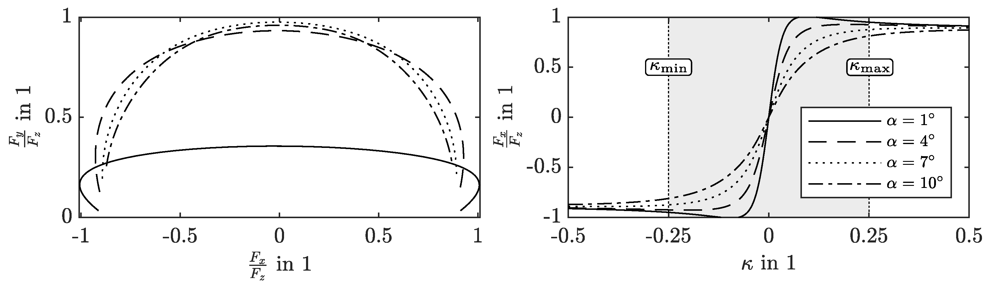
5.1. Tyre and Wheel Load Model

The Magic Formula tyre model [25] is used to map the combined lateral and longitudinal tyre forces $\left[F_{x,i}{F}_{y,i}\right]=f\left({\alpha }_i,{\kappa }_i,F_{z,i}\right)$ at each wheel. Besides the tyre sideslip angle ${\alpha }_i$ and the longitudinal tyre slip ${\kappa }_i$, [29], the wheel load $F_{z,i}$ is input to the tyre model. The wheel loads are calculated based on the longitudinal and lateral accelerations of the CoG of the vehicle, $a_x$ and $a_y$, respectively,

$$\begin{array}{cc}\hfill F_{z,1}& ={\displaystyle \frac{m}{2(l_f+l_r)}}\left(bg-h{a}_x\right)\left(1-{\displaystyle \frac{h_f}{w_{f}g}}{a}_y\right),\hfill \end{array}$$

(10a)

$$\begin{array}{cc}\hfill F_{z,2}& ={\displaystyle \frac{m}{2(l_f+l_r)}}\left(bg-h{a}_x\right)\left(1+{\displaystyle \frac{h_f}{w_{f}g}}{a}_y\right),\hfill \end{array}$$

(10b)

$$\begin{array}{cc}\hfill F_{z,3}& ={\displaystyle \frac{m}{2(l_f+l_r)}}\left(ag+h{a}_x\right)\left(1-{\displaystyle \frac{h_r}{w_{r}g}}{a}_y\right),\hfill \end{array}$$

(10c)

$$\begin{array}{cc}\hfill F_{z,4}& ={\displaystyle \frac{m}{2(l_f+l_r)}}\left(ag+h{a}_x\right)\left(1+{\displaystyle \frac{h_r}{w_{r}g}}{a}_y\right),\hfill \end{array}$$

(10d)

where h is the height of the CoG relative to the road plane, $h_f$ and $h_r$ capture the influence of vehicle roll on the load shift for the front and rear axle, and g is the acceleration of gravity. The tyre characteristics employed in this study are shown in Figure 5. In the subsequent CA, the tyre parameters are assumed to be known. Further research is required to assess the impact of parameter and model errors on the model following performance; however, a simpler tyre model with fewer parameters could be sufficient, as realized in the ESC [30].

5.2. Nonlinear Optimal Control Allocation

The objective of CA is to allocate the tyre slips ${\kappa }_i$ and RWS angle ${\delta }_r$ such that the global force and torque demands are met with the following nonlinear programming problem:

$$\begin{array}{cccc}& \underset{\kappa ,{\delta }_r}{min}\hfill & & \stackrel{\mathrm{model}\mathrm{following}\mathrm{errors}}{\overbrace{q_x{e}_x^2+q_y{e}_y^2+q_z{e}_z^2}}+\stackrel{\mathrm{actuator}\mathrm{regularization}}{\overbrace{q_{{\dot{\delta }}_r}{{\dot{\delta }}_r}^2+\sum _{i=1}^4{q}_{\kappa }{\kappa }_i^2}}\hfill \end{array}$$

(11a)

$$\begin{array}{cccc}& \mathrm{subject}\mathrm{to}\hfill & & e_x=\Sigma F_x^{\ast }\left(\kappa ,{\delta }_r\right)-{\overline{\Sigma F}}_x,\hfill \end{array}$$

(11b)

$$\begin{array}{cccc}& & & e_y=\Sigma F_y^{\ast }\left(\kappa ,{\delta }_r\right)-{\overline{\Sigma F}}_y,\hfill \end{array}$$

(11c)

$$\begin{array}{cccc}& & & e_z=\Sigma M_z^{\ast }\left(\kappa ,{\delta }_r\right)-{\overline{\Sigma M}}_z,\hfill \end{array}$$

(11d)

$$\begin{array}{cccc}& & & \left|{\kappa }_i\right|\le {\kappa }_{max}\mathrm{and}\left|{\dot{\kappa }}_i\right|\le {\dot{\kappa }}_{max},\hfill \end{array}$$

(11e)

$$\begin{array}{cccc}& & & \left|{\delta }_r\right|\le {\delta }_{r,\max }\mathrm{and}\left|{\dot{\delta }}_r\right|\le {\dot{\delta }}_{r,max},\hfill \end{array}$$

(11f)

where the steering speed ${\dot{\delta }}_r$ and the change in slip ${\dot{\kappa }}_i$ are computed based on the values of the previous evaluation of the CA and the sampling time $T_{\mathrm{CA}}$ using finite differences. $\Sigma F_x^{\ast }$, $\Sigma F_y^{\ast }$, and $\Sigma M_z^{\ast }$ represent the allocated sum of lateral and longitudinal forces and the yaw moment, respectively. By weighing the error terms $e_x$, $e_y$ and $e_z$ appropriately with weights $q_x$, $q_y$ and $q_z$, MF is achieved. Regularization terms support the optimization problem by $q_{{\dot{\delta }}_r}$ and $q_{\kappa }$ and penalize the excessive use of the actuators. Actuator constraints are considered for the RWS in (11f). To limit the longitudinal slip of the tyres, slips ${\kappa }_i$ are constrained with (11e). Wheel torques $T_{w,i}=r_l{F}_{x,i}$ are evaluated using the loaded radii $r_l$ and the longitudinal tyre forces $F_{x,i}$ obtained with the Magic Formula tyre model. The nonlinear optimization problem is formulated using CasADi [27] with an sqp-method using qpOASES [28].

6. Results and Discussion

The effectiveness of the proposed control architecture is studied concerning the following aspects: (1) the adherence of the actual vehicle handling characteristics to the reference vehicle behavior under quasi-steady-state conditions; (2) the impact of MF on the vehicle model predictability in the MPC and the subsequent path and speed tracking capabilities; (3) the impact of overactuation and MF on the stable handling envelope of the vehicle in the phase plane and in transient driving conditions. Therefore, two respective maneuvers were selected to investigate the characteristic properties of the proposed approach, as depicted in Figure 6.

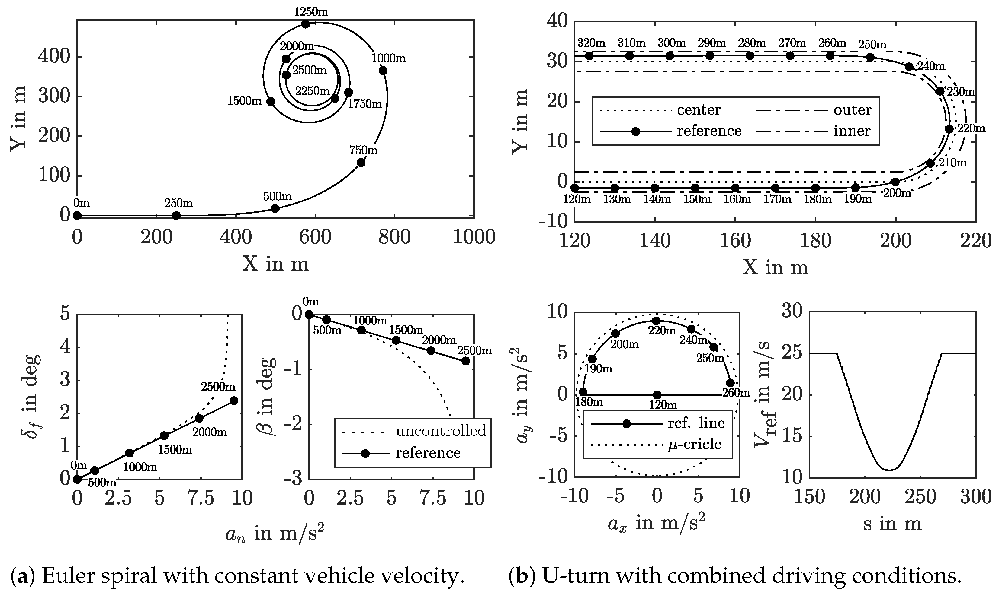
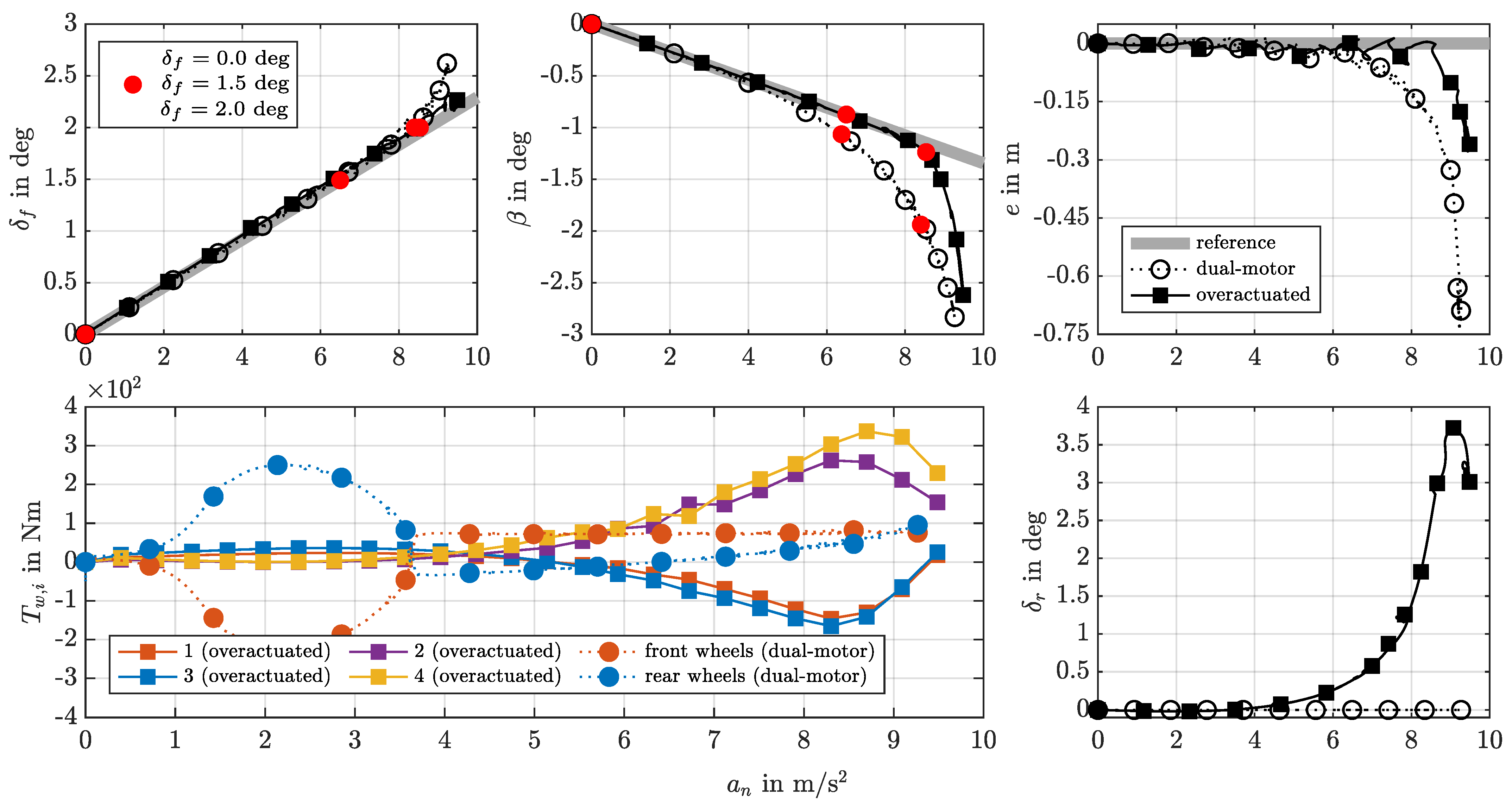
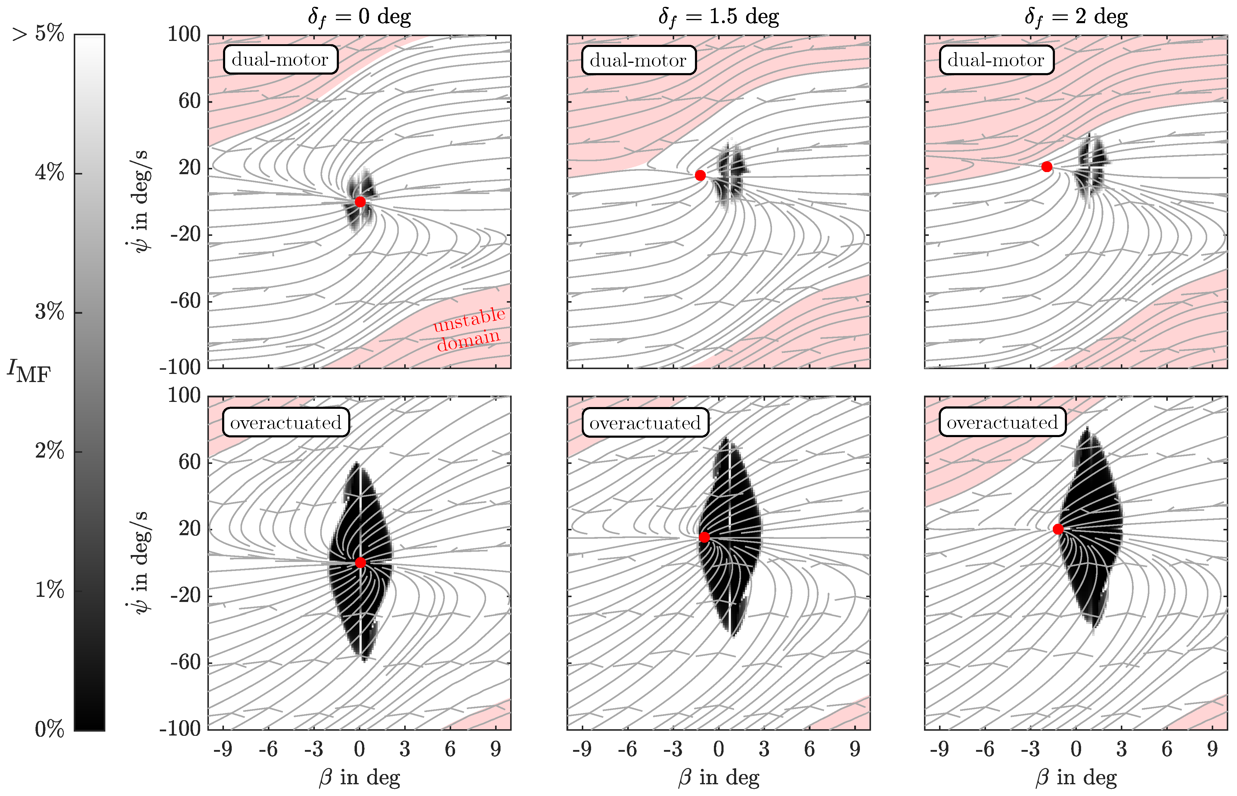
• Euler Spiral (ES). The main aims of this quasi-steady-state maneuver are to examine the effectiveness of MF in following the reference vehicle behavior and to study the respective enhancement of the MPC in path tracking at a constant $V_{\mathrm{ref}}$. Figure 6a (top) illustrates the reference path of the ES. At the bottom, the handling behavior, ${\delta }_f$ and $\beta$ over normal acceleration $a_n$ of the uncontrolled vehicle and the respective reference vehicle behavior are displayed.
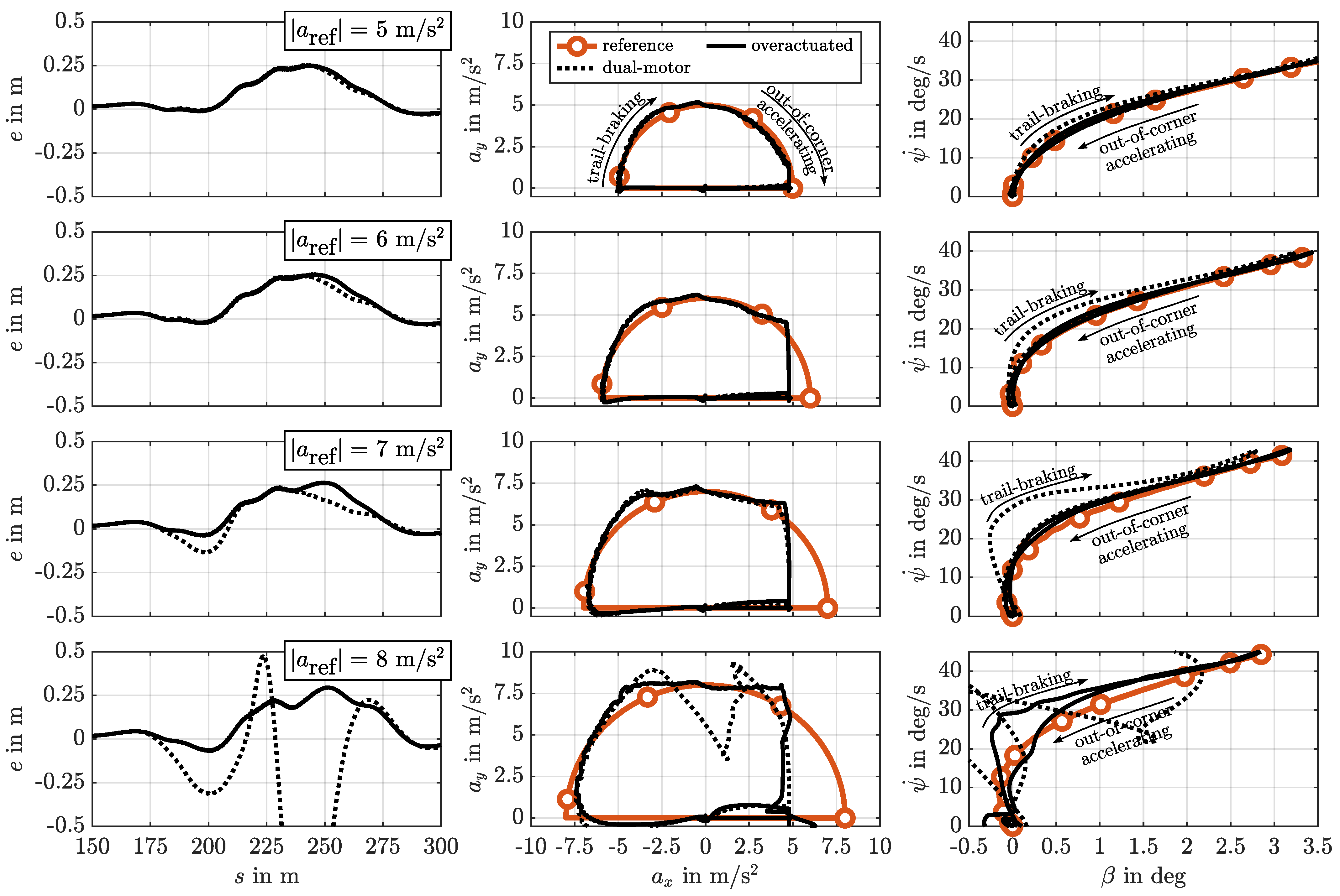
• U-Turn. The main aims of this transient maneuver are to investigate the MF and the MPC performance up to the limits of handling under pure longitudinal, pure lateral, and combined driving conditions. Figure 6b (top) shows the reference path with a left turn; at the bottom, the desired trajectory in the gg diagram and the respective velocity profile are depicted.

Two vehicle configurations are compared using a detailed multi-body vehicle model set up in Simpack; see Figure 7. Both configurations utilize the control architecture depicted in Figure 3 and differ only in the available actuator set.

The first configuration features 4WS and wheel-independent 4WD and is denoted as “overactuated” in the subsequent discussion. The second overactuated configuration features a reduced actuator set with FWS and dual-motors enabling axle-wise independent drive and is denoted as “dual-motor”. Considering the reduced actuator set, additional constraints are introduced in the CA (11) of the dual-motor configuration: ${\delta }_r=0$, $T_{w,1}=T_{w,2}$ and $T_{w,3}=T_{w,4}$.

The parameters for the LTV-MPC are given

Table 1. LTV-MPC parameters.

Name	Value		Unit
	Dual-Motor	Overactuated
N	50		-
$\Delta s$	1		$\mathrm{m}$
$T_{\mathrm{MPC}}$	0.02		$\mathrm{s}$
${\dot{\psi }}_{max}$	[13]	120	${(\mathrm{deg}/\mathrm{s})}^2$
${\beta }_0$	[13]	20	deg
$g_{\beta }$	[13]	0.175	$\mathrm{s}$
$F_{d,min}$	${\displaystyle \raisebox{1ex}{$1$}\!\left/ \!\raisebox{-1ex}{$2$}\right.}$$mg$		$\mathrm{N}$
$F_{d,max}$	$mg$		$\mathrm{N}$
${\delta }_{f,max}$	30		deg
${\dot{\delta }}_{f,max}$	30		$\mathrm{deg}/\mathrm{s}$
$q_V$	${50}^2$		-
$q_e$	${\left({\displaystyle \raisebox{1ex}{$3$}\!\left/ \!\raisebox{-1ex}{$1$}\right.}\right)}^2$		${(1/\mathrm{m})}^2$
$q_{\theta }$	${\left({\displaystyle \raisebox{1ex}{$1$}\!\left/ \!\raisebox{-1ex}{$15$}\right.}\right)}^2$		${(1/\mathrm{deg})}^2$
$q_{{\dot{\delta }}_f}$	${\left({\displaystyle \raisebox{1ex}{$4$}\!\left/ \!\raisebox{-1ex}{${\dot{\delta }}_{f,max}$}\right.}\right)}^2$		${(\mathrm{s}/\mathrm{deg})}^2$
$q_{F_d}$	${\left({\displaystyle \raisebox{1ex}{$5$}\!\left/ \!\raisebox{-1ex}{$mg$}\right.}\right)}^2$		${(1/\mathrm{N})}^2$
$q_{\dot{\psi }}$	${\left({\displaystyle \raisebox{1ex}{$25$}\!\left/ \!\raisebox{-1ex}{$10$}\right.}\right)}^2$		${(\mathrm{s}/\mathrm{deg})}^2$
$q_{\beta }$	${\left({\displaystyle \raisebox{1ex}{$25$}\!\left/ \!\raisebox{-1ex}{$23$}\right.}\right)}^2$		${(1/\mathrm{deg})}^2$

, those for the CA in

Table 2. CA parameters.

Name	Value	Unit
$T_{\mathrm{CA}}$	0.01	$\mathrm{s}$
$q^2$	$\frac{C_f{l}_f^2+C_r{l}_r^2}{C_f+C_r}$	${\mathrm{m}}^2$
${\kappa }_{max}$	0.25	-
${\dot{\kappa }}_{max}$	0.25	$1/\mathrm{s}$
${\delta }_{r,max}$	10	deg
${\dot{\delta }}_{r,max}$	10	$\mathrm{deg}/\mathrm{s}$
$q_x$	${\left({\displaystyle \raisebox{1ex}{$1$}\!\left/ \!\raisebox{-1ex}{$mg$}\right.}\right)}^2$	$N^{-2}$
$q_y$	${\left({\displaystyle \raisebox{1ex}{$1$}\!\left/ \!\raisebox{-1ex}{$mg$}\right.}\right)}^2$	$N^{-2}$
$q_z$	${\left({\displaystyle \raisebox{1ex}{$2q$}\!\left/ \!\raisebox{-1ex}{$I_{z}g$}\right.}\right)}^2$	${\left(\mathrm{N}\mathrm{m}\right)}^{-2}$
$q_{{\dot{\delta }}_r}$	${\left({\displaystyle \raisebox{1ex}{$0.03$}\!\left/ \!\raisebox{-1ex}{$10$}\right.}\right)}^2$	${(\mathrm{deg}/\mathrm{s})}^{-2}$
$q_{\kappa }$	${\left({\displaystyle \raisebox{1ex}{$0.1$}\!\left/ \!\raisebox{-1ex}{$0.3$}\right.}\right)}^2$	-
$w_f$	0.829	$\mathrm{mm}$
$w_r$	0.826	$\mathrm{mm}$
h	0.507	$\mathrm{m}$
$h_1$	h	$\mathrm{m}$
$h_2$	1.08h	$\mathrm{m}$
$r_l$	0.361	$\mathrm{m}$

and the main vehicle parameters in

Table 3. Two-wheel vehicle model parameters.

Name	Value	Unit
m	1310	$\mathrm{kg}$
$I_z$	2006	${\mathrm{kgm}}^2$
$l_f$	1.387	$\mathrm{m}$
$l_r$	1.107	$\mathrm{m}$
$C_f$	140.86	$\mathrm{k}\mathrm{N}/\mathrm{rad}$
$C_r$	176.86	$\mathrm{k}\mathrm{N}/\mathrm{rad}$

.

6.1. Euler Spiral Maneuver

The reference velocity $V_{\mathrm{ref}}$ is set to 25 m/s. The reference path features a linear increase in curvature over a distance of 2250 $\mathrm{m}$, starting from a straight line and culminating in a circle with a radius of $62.8$ m. By traveling at the constant velocity $V_{\mathrm{ref}}$, the controlled vehicle is expected to follow the path in a quasi-steady-state manner, with a linear increase in the normal acceleration $a_n$ over both the traveled distance s and time t. Consequently, the handling diagram of the vehicle is derived by tracking the reference path.

The parameters in Table 3 refer to the (linear) uncontrolled vehicle and parameterize the prediction/reference vehicle behavior for the MPC and MF in (7) and in (9), respectively. In Figure 6a (bottom), the corresponding handling diagram of the uncontrolled vehicle (dotted) and desired reference vehicle behavior (black line) is shown. Black dots relate the reference vehicle behavior to the corresponding position at the reference path.

The ES results are depicted in Figure 8. The response of the overactuated configuration is represented by solid lines with square markers, while the dual-motor configuration is represented by dotted lines with circle markers. The reference vehicle response is depicted in gray. The top row displays the steering angle ${\delta }_f$, the sideslip angle $\beta$ and the path tracking error e over the normal acceleration $a_n$. In the bottom row, the actuator utilization for the wheel torques $T_{w,i}$ and the rear-wheel steering angle ${\delta }_r$ are shown. The vehicle response will only follow the reference vehicle behavior when both MF and CA can compensate for the error terms $e_x$, $e_y$ and $e_z$ in (11). This results in a distribution of $T_{w,i}$ and ${\delta }_r$ according to (11a) that minimizes tyre slips ${\kappa }_i$.

Below $a_n\approx 4.5\mathrm{m}/{\mathrm{s}}^2$, the CA of both the overactuated and the dual-motor configuration allows for the accurate MF of the reference vehicle behavior. Since the chosen reference vehicle behavior closely matches the linear domain of the uncontrolled vehicle in this range of normal acceleration $a_n$—see Figure 6a (bottom)—minimal torque vectoring is needed to compensate for deviations. While only very small drive torques are required by the CA of the overactuated configuration (see $T_{w,i}$ in Figure 8) to match the required additional yaw moment, in the dual-motor configuration, a large drive torque split is needed, driving the rear axle and recuperating at the front axle. Consequently, the MPC tracks the reference trajectory; see ${\delta }_f$ and $\beta$ and e in Figure 8. A closer inspection of the steering angle ${\delta }_f$ and the path tracking error e reveals that the CA of the dual-motor configuration more accurately follows the reference vehicle behavior, and the MPC more precisely tracks the reference path, compared to the overactuated configuration. Prohibiting opposite signs of the front and rear drive torques in the CA (11) for the dual-motor configuration results in a slight decrease in the tracking performance and a considerable decrease in the drive torque split.

The CA in the overactuated configuration improves the MF of the reference vehicle behavior up to $a_n\approx 8.5\mathrm{m}/{\mathrm{s}}^2$ by creating an additional positive yaw moment (braking inner (left) and driving outer (right) wheels) to compensate for terminal understeer in the uncontrolled vehicle and steering the rear wheels to compensate for the otherwise increased sideslip angle $\beta$. The larger torque split for the overactuated configuration starting at around $a_n\approx 5\mathrm{m}/{\mathrm{s}}^2$ is used in combination with RWS to regulate the increase in the vehicle sideslip angle as well. The maximum normal acceleration $a_n$ is raised from $9.2\mathrm{m}/{\mathrm{s}}^2$ to $9.4\mathrm{m}/{\mathrm{s}}^2$, resulting in smaller possible quasi-steady-state cornering radii. As a result, the path tracking error e is reduced from −1 m for the dual-motor configuration to −0.25 m for the overactuated configuration at the maximum $a_n$. Consequently, the enhanced MF enlarges the applicable range of the MPC’s prediction model, improving the model predictability and resulting in lower path tracking errors e.

To improve the understanding of the root causes behind the varying MF performance and path tracking accuracy of the overactuated configuration and the dual-motor configuration, and to examine how MF facilitates the stable domain of handling under disturbances in these configurations, phase planes for both configurations are drawn at three equilibria along the ES, indicated by the red dots in Figure 8. The phase planes are calculated by evaluating the CA response at discrete points in the phase plane and assessing the resulting vehicle response. This allows for the identification and comparison of stable and unstable domains between vehicle configurations. Moreover, the RMSE metric is introduced to quantify how accurately the reference model is followed:

$$I_{\mathrm{MF}}(\beta ,\dot{\psi })=\sqrt{\frac{e_y^2(\beta ,\dot{\psi })}{{\overline{\Sigma F}}_y^2(\beta ,\dot{\psi })}+\frac{e_z^2(\beta ,\dot{\psi })}{{\overline{\Sigma M}}_z^2(\beta ,\dot{\psi })}}$$

This metric provides an assessment of the MF error in the phase plane, highlighting the deviation between the reference vehicle behavior and the actually achieved response.

In the top row of Figure 9, phase planes for constant ${\delta }_f=$ {0, 1.5, 2} deg and $T_{w,i}$ according to CA (11) are shown for the dual-motor configuration. The bottom row displays phase planes for the overactuated configuration at the same ${\delta }_f$ as in the top row and $T_{w,i}$ and ${\delta }_r$ according to CA (11). A separatrix separates the unstable domain (red) from the stable domain (white), where the trajectories converge to an equilibrium (red dots).

Evident from the phase planes is the enlarged stable domain for the overactuated configuration compared to the dual-motor configuration. These findings closely align with the enlarged controllability envelope described by [19] for TV and RWS. Moreover, the distance between the equilibrium and the separatrix remains large even in cornering conditions (${\delta }_f\ne 0$) at higher lateral accelerations for the overactuated configuration. Based on these findings, the values for the SE for the overactuated vehicle in Table 1 are chosen.

The $I_{\mathrm{MF}}$ measure is overlaid in grayscale with the indicator bar to the left of Figure 9. Darker shades indicate a close match from the controlled vehicle to the reference vehicle behavior. Conversely, lighter shades indicate an increasing MF error, where the cut-off value of $I_{\mathrm{MF}}$ is set to $5\%$. Compared to the dual-motor configuration, the overactuated configuration shows considerably better MF performance, indicated by the enlarged dark areas in the phase planes, where MF is not effective given the actuator set of the dual-motor configuration at ${\delta }_f={1.5}^{\circ }$ and $2^{\circ }$. Nevertheless, for the overactuated configuration, the stable equilibrium moves beyond the boundary of the area of accurate MF for ${\delta }_f>2^{\circ }$, aligning with the ES findings, where deviations from the reference vehicle behavior with respect to the sideslip angle $\beta$ and path tracking errors e occur for $a_n>8.5\mathrm{m}/{\mathrm{s}}^2$ for the overactuated configuration; see Figure 8.

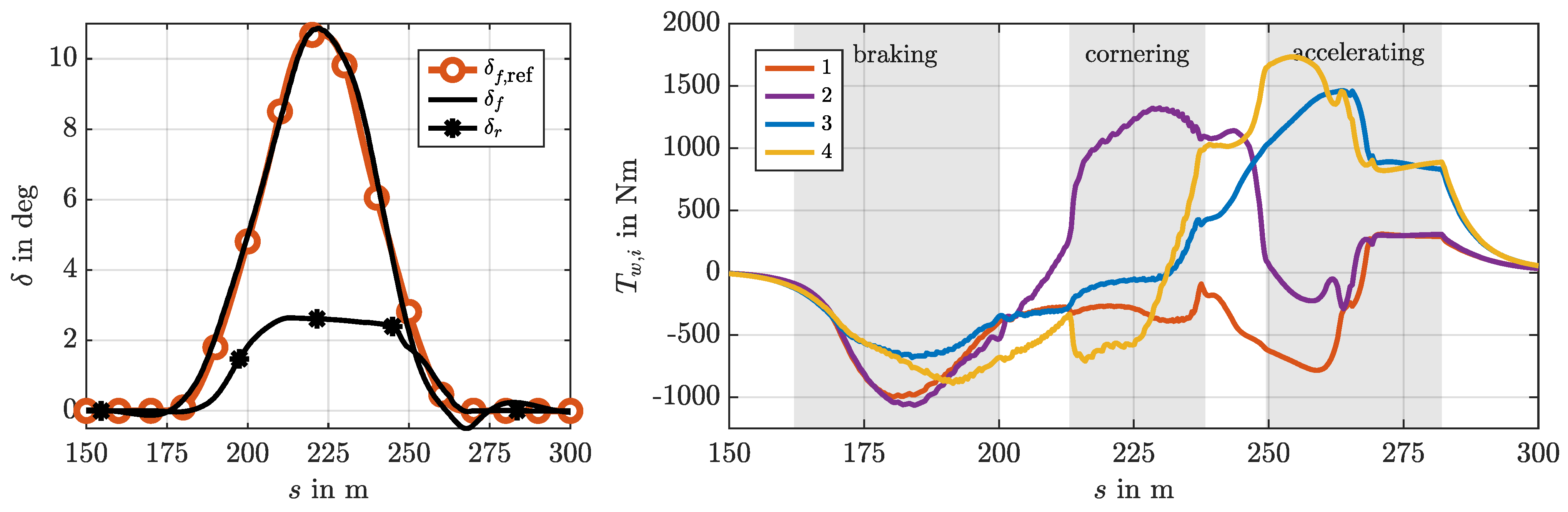
6.2. U-Turn Maneuver

The U-turn incorporates trail-braking and out-of-corner accelerating to study the stability and path tracking properties of the controlled vehicle at combined lateral and longitudinal acceleration and transient driving conditions. The reference path is calculated using the minimum curvature method [26], while the velocity profile is optimized by maximizing the combined lateral and longitudinal acceleration subject to an upper limit, defined by a reference acceleration level $|a_{\mathrm{ref}}|$.

By design, the U-turn is symmetrical with respect to the apex of the corner in both the reference path and velocity profile. Considering the linear reference vehicle behavior—see Figure 6a (bottom)—the trajectory traced in the $\beta$-$\dot{\psi }$ phase plane during the trail-braking and out-of-corner accelerating phases should be similar. Consequently, no hysteresis should appear in the phase plane.

In Figure 10, both the dual-motor and the overactuated vehicle configuration are compared. Each row in the figure corresponds to a different combined reference acceleration level $|a_{\mathrm{ref}}|$ and therefore velocity profile: $|a_{\mathrm{ref}}|=5\mathrm{m}/s^2$ in the first row, 6 $\mathrm{m}$/s2 in the second, 7 $\mathrm{m}$/s2 in the third and 8 $\mathrm{m}$/s2 in the fourth. This approach aims to explore the limits of handling and to investigate the MF error and consequently the path tracking error of the MPC for both configurations. Within each row, the first plot shows the path tracking error e, the second plot shows the gg-diagram and the third plot shows the phase plane $\beta$-$\dot{\psi }$. The solid line represents the overactuated configuration, the dashed line represents the dual-motor configuration and the reference line is shown in red with circle markers.

As $|a_{\mathrm{ref}}|$ increases, the hysteresis of the dual-motor configuration appears; see the phase plane $\beta$-$\dot{\psi }$ at the right of Figure 10. This leads to skidding under braking. The noticeable hysteresis in the phase plane of the dual-motor configuration suggests higher MF errors compared to the overactuated configuration. At lower levels of acceleration, the path tracking errors e are comparable for both configurations. However, differences become apparent for $|a_{\mathrm{ref}}|=7\mathrm{m}/s^2$ during corner entry (175 $\mathrm{m}$ to 225 $\mathrm{m}$) under trail-braking, where the dual-motor configuration saturates the front tyres, followed by skidding and steering corrections by the path tracking controller (not depicted). The increased path error e under trail-braking correlates well with the loss of model following in the trail-braking branch in the phase plane. For both configurations, starting at $|a_{\mathrm{ref}}|>5m/s^2$, a vertical line in the gg diagram at $a_x=5m/s^2$ is visible due to the $F_{d,max}$ constraint in (8e), considering the drive force limitations of the powertrain in the MPC.

At $|a_{\mathrm{ref}}|=8\mathrm{m}/s^2$, large path tracking errors e in the MPC become apparent in the dual-motor configuration due to insufficient MF. In contrast, the CA of the overactuated configuration utilizes both TV and RWS to minimize and maintain consistent hysteresis while increasing the maximum acceleration levels. The trajectories in the phase plane for this configuration remain entirely within the black areas at the apex of the curve in the phase planes depicted in Figure 9; hence, reasonable MF is provided to the MPC. Consequently, the path tracking errors e remain similar across the acceleration levels for the overactuated configuration.

In Figure 11, the actuator commands for the overactuated configuration for the U-turn at $|a_{\mathrm{ref}}|=8\mathrm{m}/s^2$ are plotted. The figure displays the steering response on the front axle ${\delta }_f$ and the rear axle ${\delta }_r$ and the wheel torques $T_{w,i}$. During the transition to straight-line running, the MPC applies negative steering corrections ${\delta }_f$ at $\approx 260m$. These corrections are apparent also in both the phase plane near the origin and the gg diagram at the maximum $a_x$ in Figure 10.

For comparison, the ideal steering response ${\delta }_{f,\mathrm{ref}}$ based on the reference vehicle behavior is plotted in the left plot of Figure 11. The generated steering command of the proposed architecture closely follows the desired steering response, indicating good MF behavior with a similar understeer gradient. The positive rear-wheel steering compensates for the otherwise larger vehicle sideslip angle $\beta$.

In the drive torque plots of the individual wheels $T_{w,i}$ in Figure 11 (right), the braking, cornering and accelerating phases are marked. During the braking phase, the CA distributes torque to the front wheels, especially to the highly loaded front right tyre ($i=2$). This aligns with the allocation criterion (11e) that aims to minimize tyre slips $\kappa$. During this phase, an additional outward-turning yaw moment is generated with the rear right wheel ($i=4$) to compensate for oversteer under braking. During the cornering phase, torques $T_{w,i}$ are predominantly used for TV, generating an inward-turning yaw moment to compensate for limit understeer. During the acceleration phase at approximately 260 $\mathrm{m}$, the MPC performs steering corrections supported by an additional inward-turning yaw moment to compensate for increased understeer during out-of-corner acceleration, visible through the positive torque split in this phase. This is followed by a longitudinal acceleration phase at 270 $\mathrm{m}$, during which the rear wheels contribute the majority of the driving torque, once again to ensure minimal slip $\kappa$.

7. Summary and Conclusions

This study explores how 4WS and wheel-independent 4WD can contribute to safe autonomous driving by improving the stable handling envelope and reducing path tracking errors under both quasi-steady-state and transient driving conditions. The proposed modular control approach separates the path and speed tracking task from the actuator allocation task. Nonlinearities such as nonlinear tyre characteristics and overactuation are considered in the computationally efficient static nonlinear optimal CA without preview, providing the reference vehicle behavior demanded by MF. Given this reference vehicle behavior, an LTV-MPC for path and speed tracking is utilized to enable rapid solver times while considering long preview horizons. Consequently, this approach also allows for simple adaptation to different actuator sets in the CA and the possibility of manual driving. In addition, MF facilitates the flexible adjustment of the reference vehicle behavior.

The simulation study demonstrates the effectiveness of TV and RWS in modifying the vehicle characteristics, i.e., accurate MF, until the full tyre–road friction potential is utilized. The results show reduced lateral errors in both quasi-steady-state and transient maneuvers up to the limits of handling compared to a dual-motor vehicle configuration. Moreover, the enlarged stable domain in the phase plane suggests enhanced robustness to state disturbances. The influence of the individual actuators on the MF performance, i.e., how well the desired reference vehicle behavior can be followed by a given set of actuators, has not yet been fully studied and may be of future interest.

Future work will involve implementing the control architecture on a prototype platform equipped with wheel-independent motors and active FWS. Initial tests conducted using a dSpace MicroAutoBox III have demonstrated an average task turnaround time of $0.25$ $\mathrm{m}$$\mathrm{s}$, with peak times reaching up to $0.5$ $\mathrm{m}$$\mathrm{s}$ for the nonlinear optimal CA. These results indicate that real-time performance is achievable under the proposed architecture.

References

1. Doerr, J.; Fröhlich, G.; Stroh, A.; Baur, M. Das elektrische Antriebssystem mit Drei-Motor-Layout im Audi E-tron S. MTZ - Mot. Z. 2020, 81, 18–27. [Google Scholar] [CrossRef]
2. Sato, S.; Inoue, H.; Tabata, M.; Inagaki, S. Integrated Chassis Control System for Improved Vehicle Dynamics. In Proceedings of the AVEC’92 (1st International Symposium on Advanced Vehicle Control), Yokohama, Japan, 14–17 September 1992. [Google Scholar]
3. Mazzilli, V.; De Pinto, S.; Pascali, L.; Contrino, M.; Bottiglione, F.; Mantriota, G.; Gruber, P.; Sorniotti, A. Integrated chassis control: Classification, analysis and future trends. Annu. Rev. Control 2021, 51, 172–205. [Google Scholar] [CrossRef]
4. Vivas-López, C.A.; Hernández-Alcantara, D.; Tudón-Martínez, J.C.; Morales-Menendez, R. Review on Global Chassis Control. IFAC Proc. Vol. 2013, 46, 875–880. [Google Scholar] [CrossRef]
5. AUDI AG. Zentraler Fahrdynamik-Rechner—Vision. 2020. Available online: https://www.audi-technology-portal.de/de/fahrwerk/fahrwerksregelsysteme/zentraler-fahrdynamikrechner-de (accessed on 12 November 2024).
6. Robert Bosch GmbH. Vehicle Dynamics Control 2.0. 2022. Available online: https://www.bosch-mobility.com/en/solutions/driving-safety/vehicle-dynamics-control/ (accessed on 12 November 2024).
7. De Novellis, L.; Sorniotti, A.; Gruber, P.; Shead, L.; Ivanov, V.; Hoepping, K. Torque Vectoring for Electric Vehicles with Individually Controlled Motors: State-of-the-Art and Future Developments. World Electr. Veh. J. 2012, 5, 617–628. [Google Scholar] [CrossRef]
8. Meitinger, K.H. New Chassis Systems—Das Fahrwerk des AUDI R8 e-Tron (The Chassis of the AUDI R8 e-Tron). In Proceedings of the 7th International Munich Chassis Symposium, Munich, Germany, 14–15 June 2016; pp. 89–102. [Google Scholar] [CrossRef]
9. De Novellis, L.; Sorniotti, A.; Gruber, P. Wheel Torque Distribution Criteria for Electric Vehicles With Torque-Vectoring Differentials. IEEE Trans. Veh. Technol. 2014, 63, 1593–1602. [Google Scholar] [CrossRef]
10. Hoffmann, G.M.; Tomlin, C.J.; Montemerlo, M.; Thrun, S. Autonomous Automobile Trajectory Tracking for Off-Road Driving: Controller Design, Experimental Validation and Racing. In Proceedings of the 2007 American Control Conference, New York, NY, USA, 11–13 July 2007; pp. 2296–2301. [Google Scholar] [CrossRef]
11. Keviczky, T.; Falcone, P.; Borrelli, F.; Asgari, J.; Hrovat, D. Predictive control approach to autonomous vehicle steering. In Proceedings of the 2006 American Control Conference, Minneapolis, MN, USA, 14–16 June 2006; p. 6. [Google Scholar] [CrossRef]
12. Beal, C.E.; Gerdes, J.C. Model Predictive Control for Vehicle Stabilization at the Limits of Handling. IEEE Trans. Control Syst. Technol. 2013, 21, 1258–1269. [Google Scholar] [CrossRef]
13. Erlien, S.M.; Fujita, S.; Gerdes, J.C. Safe Driving Envelopes for Shared Control of Ground Vehicles. IFAC Proc. Vol. 2013, 46, 831–836. [Google Scholar] [CrossRef]
14. Funke, J.; Brown, M.; Erlien, S.M.; Gerdes, J.C. Collision Avoidance and Stabilization for Autonomous Vehicles in Emergency Scenarios. IEEE Trans. Control Syst. Technol. 2017, 25, 1204–1216. [Google Scholar] [CrossRef]
15. Bobier-Tiu, C.G.; Beal, C.E.; Kegelman, J.C.; Hindiyeh, R.Y.; Gerdes, J.C. Vehicle control synthesis using phase portraits of planar dynamics. Veh. Syst. Dyn. 2019, 57, 1318–1337. [Google Scholar] [CrossRef]
16. Gao, Y.; Gray, A.; Tseng, H.E.; Borrelli, F. A tube-based robust nonlinear predictive control approach to semiautonomous ground vehicles. Veh. Syst. Dyn. 2014, 52, 802–823. [Google Scholar] [CrossRef]
17. Mokhiamar, O.; Abe, M. How the four wheels should share forces in an optimum cooperative chassis control. Control Eng. Pract. 2006, 14, 295–304. [Google Scholar] [CrossRef]
18. Metzler, M.; Tavernini, D.; Sorniotti, A.; Gruber, P. An explicit nonlinear MPC approach to vehicle stability control. In Proceedings of the AVEC ’18 14th International Symposium on Advanced Vehicle Control, Beijing, China, 16–20 July 2018; p. 6. [Google Scholar]
19. Horiuchi, S. Evaluation of chassis control method through optimisation-based controllability region computation. Veh. Syst. Dyn. 2012, 50, 19–31. [Google Scholar] [CrossRef]
20. Mokhiamar, O.; Abe, M. Simultaneous Optimal Distribution of Lateral and Longitudinal Tire Forces for the Model Following Control. J. Dyn. Syst. Meas. Control 2005, 126, 753–763. [Google Scholar] [CrossRef]
21. Chatzikomis, C.; Sorniotti, A.; Gruber, P.; Bastin, M.; Shah, R.M.; Orlov, Y. Torque-Vectoring Control for an Autonomous and Driverless Electric Racing Vehicle with Multiple Motors. SAE Int. J. Veh. Dyn. Stability NVH 2017, 1, 338–351. [Google Scholar] [CrossRef]
22. Falcone, P.; Tufo, M.; Borrelli, F.; Asgari, J.; Tseng, H.E. A linear time varying model predictive control approach to the integrated vehicle dynamics control problem in autonomous systems. In Proceedings of the 2007 46th IEEE Conference on Decision and Control, New Orleans, LA, USA, 12–14 December 2007; pp. 2980–2985. [Google Scholar] [CrossRef]
23. Gordon, T.; Howell, M.; Brandao, F. Integrated Control Methodologies for Road Vehicles. Veh. Syst. Dyn. 2003, 40, 157–190. [Google Scholar] [CrossRef]
24. Johansen, T.A.; Fossen, T.I. Control allocation—A survey. Automatica 2013, 49, 1087–1103. [Google Scholar] [CrossRef]
25. Pacejka, H.B. Tire and Vehicle Dynamics, 2nd ed.; Number 372 in SAE-R; SAE International: Warrendale, PA, USA, 2006. [Google Scholar]
26. Sedlacek, T. Minimum-Time Optimal Control for Automotive Vehicles. Ph.D. Thesis, Technischen Universität München, München, Germany, 2021. [Google Scholar]
27. Andersson, J.A.E.; Gillis, J.; Horn, G.; Rawlings, J.B.; Diehl, M. CasADi: A software framework for nonlinear optimization and optimal control. Math. Program. Comput. 2019, 11, 1–36. [Google Scholar] [CrossRef]
28. Ferreau, H.; Kirches, C.; Potschka, A.; Bock, H.; Diehl, M. qpOASES: A parametric active-set algorithm for quadratic programming. Math. Program. Comput. 2014, 6, 327–363. [Google Scholar] [CrossRef]
29. Lugner, P. (Ed.) Vehicle Dynamics of Modern Passenger Cars; CISM International Centre for Mechanical Sciences; Springer International Publishing: Cham, Switzerland, 2019; Volume 582. [Google Scholar] [CrossRef]
30. Van Zanten, A.T.; Erhardt, R.; Pfaff, G.; Kost, F.; Hartmann, U.; Ehret, T. Control aspects of the bosch-VDC. In Proceedings of the AVEC’96 (2nd International Symposium on Advanced Vehicle Control), Aachen University of Technology, Aachen, Germany, 24–28 June 1996. [Google Scholar]
Figure 1. Impact of integrated control on friction circle; adapted from [2].
Applsci 14 10718 g001
Figure 2. Vehicle motion controller as part of a multilayered upstream control architecture [3].
Applsci 14 10718 g002
Figure 3. Control architecture composed of LTV-MPC for path and speed tracking, MF for global demand generation and CA. Inputs: segment of the reference path via V ref and ρ , along with current tracking errors e and θ and vehicle state. Outputs: wheel torques T w and steering angles δ f and δ r .
Applsci 14 10718 g003
Figure 4. (a) Two-wheel vehicle model used in MPC and MF. (b) Four-wheel vehicle model used in CA.
Applsci 14 10718 g004
Figure 5. Left plot shows the normalized lateral tyre force F y F z over the normalized longitudinal tyre force F x F z for various tyre sideslip angles α . Right plot shows the normalized longitudinal force F x F z over the longitudinal tyre slip κ for various tyre side slip angles α , with the gray area defining the slip constraint for the CA.
Applsci 14 10718 g005
Figure 6. (a) Euler spiral path (top) and handling diagram for uncontrolled vehicle and reference vehicle behavior (bottom). (b) U-turn path (top) and desired acceleration in gg diagram with corresponding reference vehicle velocity (bottom).
Applsci 14 10718 g006
Figure 7. Multi-body vehicle model.
Applsci 14 10718 g007
Figure 8. Euler spiral maneuver simulated with the overactuated and dual-motor configurations. Linear (reference) vehicle behavior given in gray. Top row shows front steering angle δ f , vehicle sideslip angle β and path tracking error e characteristics over a n . Bottom row shows actuator usage for wheel torques T w , i and rear-wheel steering angle δ r .
Applsci 14 10718 g008
Figure 9. Phase planes at varying FWS angles corresponding to the dual-motor and overactuated configurations at V = 25 m / s . Stable and unstable regions are shown in white and red, respectively. The I MF measure is overlaid in grayscale. Red dots indicate stable equilibria corresponding to Figure 8 (top).
Applsci 14 10718 g009
Figure 10. U-turn maneuver at varying reference acceleration levels | a ref | . Results are shown for the dual-motor configuration (dotted), the overactuated configuration (solid) and the reference trajectory (red with circle markers).
Applsci 14 10718 g010
Figure 11. U-turn actuator commands at reference acceleration level | a ref | = 8 m / s 2 for the overactuated vehicle configuration.
Applsci 14 10718 g011