Optimal Configuration of Soft Open Point and Energy Storage Based on Snowflake-Shaped Grid Characteristics and Sensitivity Analysis

Abstract

With the continuous penetration of flexible resources, the distribution network is gradually forming a two-way interactive supply and demand relationship with the transmission network and users. The deployment of soft open point (SOP) and energy storage represents a crucial strategy for voltage regulation and power flow control in distribution networks. This article puts forth a methodology for optimizing the configuration of SOP and energy storage based on the characteristics of the snowflake-shaped grid and sensitivity analysis. Firstly, the location of the SOP is determined based on the characteristics of the interconnection nodes between snowflake websites. Secondly, the voltage sensitivity analysis is employed to identify nodes that have a significant impact on the system voltage distribution, thereby enabling the selection of an optimal energy storage site. Subsequently, a multi-objective optimization configuration model for SOP and energy storage is established, taking into account the economic efficiency and load balancing of the power grid. Finally, the method is verified using a snowflake-shaped grid in Tianjin. In comparison with the plan that solely considers the economic aspects of the power grid, the method proposed in this article can reduce the degree of load balancing by 50.93% while simultaneously increasing the annual comprehensive cost by only 24.35%.

1. Introduction

The ongoing acceleration of the construction process of China’s new power system, which is dominated by new energy, has resulted in notable shifts in the circumstances and responsibilities confronting the distribution network within the context of the new power system [1,2]. These changes can be attributed to a number of factors, including the high proportion of distributed new energy access, the accelerated substitution of electric energy, the enhanced load interaction, and the advancement of power electronic equipment. The distribution network represents a pivotal component of the new power system, serving as the conduit for the direct provision of power to end users. The traditional distribution network is characterized by a relatively singular function, with a top–down unidirectional supply and demand relationship with the transmission network and users. As a consequence of the ongoing integration of flexible resources, including distributed power sources, energy storage systems, and electric vehicles, the distribution network will evolve towards a two-way interactive supply and demand relationship with the transmission network and users. This will result in a gradual shift in the operation and management of the power grid towards a “source load interaction” mode [3,4].

In this context, in response to the shortcomings of the widely used grid structure in terms of scalability and load transfer in China, some scholars have proposed the snowflake-shaped grid structure [5], which has the characteristics of high flexibility, high controllability, and strong load transfer ability. This structure is better able to adapt to the needs of power grid development in the new situation than the grid structure that has been widely used until now. It is of particular importance to investigate the allocation of flexible resources in order to fully capitalize on the advantages of the snowflake-shaped grid.

SOP represents a novel type of intelligent distribution device that is designed to supplant traditional interconnection switches. It exhibits the hallmarks of continuous and precise power control, balancing the load between feeders [6], and the capacity to effectively adapt to changes brought about by flexible resource access. To date, research into SOP has yielded certain results. In [7], a SOP planning method for active distribution networks is proposed, which considers the influence of the access mode between feeder loops and reliability. This method has the potential to significantly enhance the reliability and stability of the distribution network. In [8], an optimal configuration method of SOP for an active distribution network considering the characteristics of distributed Generation is proposed. This method fully leverages the role of SOP in smoothing load fluctuations and peak shaving, effectively reducing the operating costs of distribution networks. In [9], an improvement method for the photovoltaic consumption capacity of an AC/DC hybrid distribution network considering the time-of-use electricity price and SOP collaboration is proposed. Through the rational allocation of SOP, the rich demand response resources on the user side are fully utilized, thereby greatly improving the load balancing degree of the distribution network.

With the integration of renewable energy, the application scenarios of energy storage in distribution networks are gradually becoming more diverse. Considering the limitation of the charge capacity of energy storage batteries, the charging and discharging power of energy storage systems cannot flexibly adapt to changes in the real-time status of the distribution network. Accordingly, energy storage systems typically regulate the charging and discharging power in accordance with pre-established scheduling strategies. SOP has the characteristics of a fast response speed and smooth power adjustment, and it can perform real-time power adjustment and compensate for the optimization effect of energy storage systems to a certain extent. A substantial body of research has been devoted to the coordinated operation optimization of energy storage systems with other dispatchable resources [10,11,12]. However, relatively little research has been conducted on the coordination between energy storage systems and SOP. In [13], the coordinated operational relationship between an energy storage system and SOP was considered, and the role of the energy storage system and SOP in improving the operational economy of active distribution networks from the perspective of optimizing the configuration was studied. The energy storage system transfers energy over time and adjusts the power in space in conjunction with the SOP, which will greatly optimize the operation status of the distribution network, thus ensuring the safe and economical operation of the distribution network.

This article proposes an SOP and energy storage optimization configuration method for the snowflake-shaped grid. Firstly, the selection of SOP sites is achieved through the interconnection nodes between snowflake websites, which greatly reduces the difficulty of solving SOP optimization configurations, based on the analysis of the snowflake-shaped grid structure. Secondly, site selection for energy storage is achieved based on sensitivity analysis methods. Subsequently, a multi-objective optimization configuration model for SOP and energy storage is developed, considering the economic efficiency and load balancing of the power grid, in order to achieve the best capacity for SOP and energy storage. Finally, the efficacy of the proposed model and method is validated using actual data from the snowflake-shaped grid.

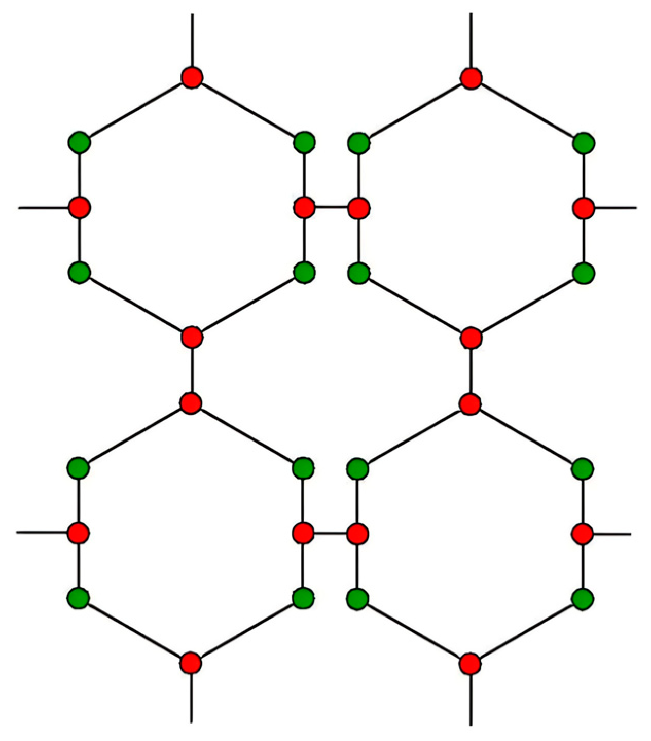
2. SOP Siting Based on the Characteristics of a Snowflake-Shaped Grid Structure

The snowflake-shaped grid structure is based on a 10 kV ring cage, which serves as the core node. This is composed of eight 10 kV lines originating from four substations (or six lines from three substations), which form an independent feeder cluster. The purpose of this cluster is to provide power to the enclosed power supply area. Each substation is equipped with two 10 kV outgoing lines, each with one inter-station and one intra-station connection. These lines operate in an open-loop configuration. Eight (or six) lines are enclosed to form a snowflake-shaped area. The structural design of the snowflake-shaped grid embodies the concept of combined planning, which is consistent with the Constructive Law.

The schematic diagram of the four-station snowflake-shaped grid is presented in Figure 1. The snowflake-shaped grid comprises four inter-station contact points and four intra-station contact points. The inter-station contact points are defined as key nodes, marked with red dots. The internal contact points are defined as secondary key nodes, marked with green dots. The other ring network nodes are defined as general nodes, which together with the 10 kV lines form the edges of the snowflake-shaped grid.

The traditional 10 kV grid structure is oriented towards a singular line and lacks an analytical focus on the network constituted by the lines. The snowflake-shaped grid introduces the concept of a feeder cluster, which is defined as a collection of multiple 10 kV lines connected through specific relationships. In terms of its physical configuration, each line is connected to two other lines, and the network structure is characterized by a high degree of simplicity and clarity and a lack of redundancy. In terms of functionality, each line is capable of transferring a load through the other seven lines. The grid structure is safe, reliable, and flexible in operation, making it a highly inclusive and adaptable power grid structure.

In regions with elevated expectations regarding the dependability of the power supply, it is likewise feasible to reinforce the interconnection between feeder clusters, facilitate the load transfer between feeder clusters, construct a more substantial resource allocation platform, and establish a vast snowflake-shaped grid structure comprising small snowflakes as the fundamental unit, as illustrated in Figure 2.

The preceding analysis demonstrates that the snowflake-shaped grid exhibits enhanced stability and reliability compared to the traditional 10 kV distribution network. Its distinctive grid structure endows it with robust load transfer capabilities, enabling it to effectively adapt to a high proportion of flexible resource access [5]. To date, the snowflake-shaped grid has been implemented in a number of demonstration areas, including the High-End Equipment Industrial Park in Beichen District, Tianjin, the Hexi National Game Village, and the Binhai New Area Ecological City Tourism Zone.

SOP is capable of achieving rapid and dynamic control of active and reactive power flows; therefore, its site selection must take into account the characteristics and requirements of the power flow within the power grid [14]. In light of the aforementioned analysis of the snowflake-shaped grid structure, it can be concluded that the inter-station connection nodes in the snowflake-shaped grid serve as the hub for the power flow between different lines, thereby meeting the site selection conditions of SOP. The installation of SOP at inter-station communication nodes serves to balance loads and optimize system voltage distribution.

3. Energy Storage Siting Based on Sensitivity Analysis

The selection of an energy storage site is based on sensitivity analysis, which expands the power balance equation of system nodes in accordance with Taylor’s first-order expansion. This is achieved by setting the reactive power change $\Delta Q=0$ and the active power change $\Delta P=0$ in order to obtain the relationship between voltage change $\Delta V$, $\Delta P$, and $\Delta Q$.

$$\mathsf{\Delta }V={\left({\displaystyle \frac{\partial \mathsf{\Delta }P}{\partial V}}-{\displaystyle \frac{\partial \mathsf{\Delta }P}{\partial \theta }}{\left({\displaystyle \frac{\partial \mathsf{\Delta }Q}{\partial \theta }}\right)}^{-1}{\displaystyle \frac{\partial \mathsf{\Delta }Q}{\partial V}}\right)}^{-1}\mathsf{\Delta }P$$

(1)

$$\mathsf{\Delta }V={\left({\displaystyle \frac{\partial \mathsf{\Delta }Q}{\partial V}}-{\displaystyle \frac{\partial \mathsf{\Delta }Q}{\partial \theta }}{\left({\displaystyle \frac{\partial \mathsf{\Delta }P}{\partial \theta }}\right)}^{-1}{\displaystyle \frac{\partial \mathsf{\Delta }P}{\partial V}}\right)}^{-1}\mathsf{\Delta }Q$$

(2)

In (1) and (2), V and $\theta$ are the voltage amplitude and phase angle, respectively.

Further expansion of (1) and (2) leads to the following equation:

$${\left[\Delta V_1\cdots \Delta V_j\cdots \Delta V_{(n-1)}\right]}^T=\left[\begin{array}{ccccc}{\lambda }_{11}& \cdots & {\lambda }_{1i}& \cdots & {\lambda }_{1(n-1)}\\ ⋮& & ⋮& & ⋮\\ {\lambda }_{j1}& \cdots & {\lambda }_{ji}& \cdots & {\lambda }_{j(n-1)}\\ ⋮& & ⋮& & ⋮\\ {\lambda }_{(n-1)1}& \cdots & {\lambda }_{(n-1)i}& \cdots & {\lambda }_{(n-1)(n-1)}\end{array}\right]\left[\begin{array}{c}\Delta P_1\\ ⋮\\ \Delta P_i\\ ⋮\\ \Delta P_{(n-1)}\end{array}\right]$$

(3)

$${\left[\Delta V_1\cdots \Delta V_j\cdots \Delta V_{(n-1)}\right]}^T=\left[\begin{array}{ccccc}{\gamma }_{11}& \cdots & {\gamma }_{1i}& \cdots & {\gamma }_{1(n-1)}\\ ⋮& & ⋮& & ⋮\\ {\gamma }_{j1}& \cdots & {\gamma }_{ji}& \cdots & {\gamma }_{j(n-1)}\\ ⋮& & ⋮& & ⋮\\ {\gamma }_{(n-1)1}& \cdots & {\gamma }_{(n-1)i}& \cdots & {\gamma }_{(n-1)(n-1)}\end{array}\right]\left[\begin{array}{c}\Delta Q_1\\ ⋮\\ \Delta Q_i\\ ⋮\\ \Delta Q_{(n-1)}\end{array}\right]$$

(4)

In (3) and (4), n is the number of nodes. $\Delta V_j$ is the voltage variation of node j. $\Delta P_i$ and $\Delta Q_i$ represent the active power change and reactive power change of node i, respectively. ${\lambda }_{ij}$ and ${\gamma }_{ij}$ are the sensitivity of the active power change and the reactive power change of node i to the voltage of node j, respectively. The matrix composed of ${\lambda }_{ij}$ and ${\gamma }_{ij}$ is the sensitivity matrix of active and reactive power, respectively.

Considering the impact of power changes at a certain node on the voltage of each node in the distribution system, the sensitivity of power changes at node i to the voltage at node j in the system is as follows.

$${\delta }_{ji}={\omega }_1{\lambda }_{ji}+{\omega }_2{\gamma }_{ji}$$

(5)

In (5), ${\omega }_1$ and ${\omega }_2$ are the sensitivity weight coefficients for active and reactive voltage, respectively, and ${\omega }_1+{\omega }_2=1$.

The calculation method for the weight coefficients A and B will be explained below. The ideal point method [15] represents a comprehensive evaluation approach that is capable of objectively, fairly, and reasonably assessing the evaluated object. In the ideal point method, assuming there are m evaluation indicators, the optimal value of each indicator is defined as the ideal point $X^{\ast }=(x_1^{\ast },x_2^{\ast },\cdots ,x_m^{\ast })$, and the actual value of the ith evaluated object for each indicator is ${\mathit{X}}_i=(x_{i1},x_{i2},\cdots ,x_{im})$. The optimality of the ith evaluated object among all evaluated objects is evaluated using the weighted distance between $X_i$ and the ideal point $X^{*}$. In the majority of cases, the Euclidean distance is employed, which is defined as follows.

$$y_i=\sum _{j=1}^m{\omega }_j{(x_{ij}-x_j^{\ast })}^2$$

(6)

In (6), $y_i$ is the Euclidean distance of the ith evaluated object. ${\omega }_j$ is the weight coefficient of the jth evaluation indicator. $x_{ij}$ is the calculated value of the jth evaluation indicator for the ith evaluated object. $x_j^{*}$ is the ideal point for the jth evaluation metric.

Let the active power and the reactive power of the load grow in a certain proportion [16] in the following manner.

$${\displaystyle \frac{\mathsf{\Delta }{Q}_i}{\mathsf{\Delta }{P}_i}}=\tan {\phi }_i$$

(7)

In (7), ${\phi }_i$ is the power factor angle of load growth, used to describe the proportional relationship of load growth.

The load increment of the system is assumed to be as follows.

$$\{\begin{array}{c}\mathsf{\Delta }{P}_i=m_1\mathrm{d}{P}_i\\ \mathsf{\Delta }{Q}_i=m_2\mathrm{d}{Q}_i\end{array}$$

(8)

In (8), $m_1$ is the active power growth coefficient. $m_2$ is the reactive power growth coefficient.

Substituting (8) into (7) yields (9).

$${\displaystyle \frac{m_2\mathrm{d}{Q}_i}{m_1\mathrm{d}{P}_i}}={\displaystyle \frac{\sin {\phi }_i}{\cos {\phi }_i}}$$

(9)

Substituting (9) into (6) yields (10).

$$\{\begin{array}{c}{\omega }_1={\displaystyle \frac{1}{m_1}}\\ {\omega }_2={\displaystyle \frac{1}{m_2}}\end{array}$$

(10)

Taking into account the weighting coefficient constraints, (11) can be obtained.

$$\{\begin{array}{c}{\omega }_1={\displaystyle \frac{\cos {\phi }_i}{\sin {\phi }_i+\cos {\phi }_i}}\\ {\omega }_2={\displaystyle \frac{\sin {\phi }_i}{\sin {\phi }_i+\cos {\phi }_i}}\end{array}$$

(11)

It can be observed that an increase in the sensitivity value will result in a proportional increase in the impact of power fluctuations on the system voltage. It can therefore be concluded that connecting energy storage to nodes with higher sensitivity values will result in an effective improvement in the voltage distribution of both the aforementioned nodes and the entire system. Accordingly, the selection of an energy storage site may be based on the calculated sensitivity values.

4. SOP and Energy Storage Optimization Configuration Model

4.1. Objective Function

This article constructs the objective function based on the principle of balancing the economic efficiency of the power grid and load balancing. The expression is as follows:

$$\min f=\alpha f_1^{nor}+\beta f_2^{nor}$$

(12)

$$f_1^{nor}={\displaystyle \frac{f_1-f_1^{\min }}{f_1^{\max }-f_1^{\min }}}$$

(13)

$$f_2^{nor}={\displaystyle \frac{f_2-f_2^{\min }}{f_2^{\max }-f_2^{\min }}}$$

(14)

In (12)–(14), $f_1$ represents the annual comprehensive cost of SOP and energy storage, and $f_2$ represents the load balancing degree. $f_1^{nor}$ and $f_2^{nor}$ are the normalized values of $f_1$ and $f_2$, respectively. $\alpha$ and $\beta$ are the weights of $f_1$ and $f_2$ in the objective function, respectively, and $\alpha +\beta =1$. $f_1^{\max }$ and $f_2^{\max }$ are the maximum values obtained when $f_1$ and $f_2$ are solved separately. $f_1^{\min }$ and $f_2^{\min }$ are the minimum values obtained when solving $f_1$ and $f_2$ separately.

The specific composition of the annual comprehensive cost of SOP and energy storage is as follows.

$$f_1=C_{SOP}^{inv}+C_{SOP}^{ope}+C_{ES}^{inv}+C_{ES}^{ope}+C^{loss}$$

(15)

$$C_{SOP}^{inv}={\displaystyle \frac{d_1{(1+d_1)}^{y_1}}{{(1+d_1)}^{y_1}-1}}{\displaystyle \sum _{k=1}^{N_{SOP}}{c}_{k,SOP}{S}_{k,SOP}}$$

(16)

$$C_{SOP}^{inv}={\displaystyle \frac{d_1{(1+d_1)}^{y_1}}{{(1+d_1)}^{y_1}-1}}{\displaystyle \sum _{k=1}^{N_{SOP}}{c}_{k,SOP}{S}_{k,SOP}}$$

(17)

$$C_{ES}^{inv}={\displaystyle \frac{d_2{(1+d_2)}^{y_2}}{{(1+d_2)}^{y_2}-1}}{\displaystyle \sum _{k=1}^{N_{ES}}{c}_{k,ES}{S}_{k,ES}}$$

(18)

$$C_{ES}^{ope}={\displaystyle \sum _{k=1}^{N_{ES}}{c}_{k,ES}^{ope}{P}_{k,ES}}$$

(19)

$$C^{loss}=365c{\displaystyle \sum _{t=1}^{N_t}({\displaystyle \sum _{ij\in {\mathsf{\Omega }}_b}{r}_{ij}{I}_{ij,t}^2}+{\displaystyle \sum _{i=1}^{N_i}{P}_{SOP,i,t}^{loss}})}$$

(20)

In (15)–(20), $C_{SOP}^{inv}$ is the investment cost of SOP. $C_{SOP}^{ope}$ is the cost of SOP operation and maintenance. $C_{ES}^{inv}$ is the investment cost of energy storage. $C_{ES}^{ope}$ is the cost of energy storage operation and maintenance. $C^{loss}$ is the cost of power supply loss in the distribution network. $d_1$ is the SOP investment discount rate. $y_1$ is the service life of SOP. $N_{SOP}$ is the number of SOP installations to be selected. $c_{k,SOP}$ is the unit capacity investment cost of the kth SOP. $S_{k,SOP}$ is the capacity of the kth SOP. $\eta$ is the coefficient of operation and maintenance costs. $d_2$ is the discount rate for energy storage investment. $y_2$ is the service life of energy storage. N_ES is the number of energy storage installations to be selected. $c_{k,ES}$ is the investment cost per unit capacity of the kth energy storage. $S_{k,ES}$ is the capacity of the kth energy storage. $c_{k,ES}^{ope}$ is the operating and maintenance cost of the kth energy storage unit rated power. $P_{k,ES}$ is the rated power of the kth energy storage. c is the electricity price. $N_t$ is the total number of time periods. ${\mathsf{\Omega }}_b$ is the collection of all branches in the distribution system. $r_{ij}$ is the resistance of the branch ij. $I_{ij,t}$ is the current amplitude of branch ij during the tth time period. $N_i$ is the total number of nodes in the distribution system. $P_{SOP,i,t}^{loss}$ is the active power loss of SOP at node i during the tth time period.

The expression for load balancing degree $f_2$ is as follows.

$$P_{balance}={\displaystyle \sum _{i=1}^{N_s}\left|{\displaystyle \sum _{t=1}^{N_t}{P}_{source,i,t}}-P_{source,ave}\right|}$$

(21)

$$P_{source,ave}={\displaystyle \frac{{\displaystyle \sum _{t=1}^{N_t}{\displaystyle \sum _{i=1}^{N_s}{P}_{source,i,t}}}}{N_s}}$$

(22)

In (21) and (22), $N_s$ represents the total number of power nodes in the distribution system. $P_{source,i,t}$ is the active power output of the ith power node during the tth time period. $P_{source,ave}$ is the average active power output of all power nodes in the distribution system over one day.

4.2. Constraint Condition

4.2.1. System Power Flow Constraints

In (23)–(28), $r_{ij}$ and $x_{ij}$ are the resistance and the reactance of branch ij, respectively. $P_{ij}$ is the active power flowing from node i to node j on the branch, and $Q_{ij}$ is the reactive power flowing from node i to node j on the branch. $P_i$ is the sum of the active power injected into node i. $P_i^{ES}$ is the active power injected by the energy storage at node i. $P_i^{SOP}$ is the active power injected by the SOP at node i. $P_i^{LOAD}$ is the active power consumed by the load at node i. $Q_i$ is the sum of the reactive power injected at node i. $Q_i^{ES}$ is the reactive power injected by the energy storage at node i. $Q_i^{SOP}$ is the reactive power injected by the SOP at node i. $Q_i^{LOAD}$ is the reactive power consumed by the load at node i.

$$\sum _{ji\in {\mathsf{\Omega }}_{\mathrm{b}}}(P_{t,ji}-r_{ji}{I}_{t,ij}^2)+P_{t,i}=\sum _{ik\in {\mathsf{\Omega }}_{\mathrm{b}}}{P}_{t,ik}$$

(23)

$$\sum _{ji\in {\mathsf{\Omega }}_{\mathrm{b}}}(Q_{t,ji}-x_{ji}{l}_{t,ij}^2)+Q_{t,i}=\sum _{ik\in {\mathsf{\Omega }}_{\mathrm{b}}}{Q}_{t,ik}$$

(24)

$$U_{t,i}^2-U_{t,j}^2+(r_{ij}^2+x_{ij}^2)l_{t,ij}^2-2(r_{ij}{P}_{t,ij}+x_{ij}{Q}_{t,ij})=0$$

(25)

$$I_{t,ij}^2{U}_{t,i}^2=P_{t,ij}^2+Q_{t,ij}^2$$

(26)

$$P_{t,i}=P_{t,i}^{\mathrm{ES}}+P_{t,i}^{\mathrm{SOP}}-P_{t,i}^{\mathrm{LOAD}}$$

(27)

$$Q_{t,i}=Q_{t,i}^{\mathrm{ES}}+Q_{t,i}^{\mathrm{SOP}}-Q_{t,i}^{\mathrm{LOAD}}$$

(28)

Equation (25) represents a quadratic nonlinear constraint, which can be transformed into a second-order cone constraint form under the conditions that the objective function is strictly increasing and the node load is not constrained by an upper bound [17].

$${\Vert \begin{array}{c}2P_{ij}\\ 2Q_{ij}\\ i_{ij}-u_i\end{array}\Vert }_2\le i_{ij}+u_i$$

(29)

4.2.2. System Operation Constraints

In (30) and (31), $\underset{¯}{U}$ and $\overline{U}$ are the minimum and maximum allowable node voltage values of the system, respectively. $\overline{I}$ is the maximum allowable branch current value of the system.

$${(\underset{¯}{U})}^2\le U_i^2\le {(\overline{U})}^2$$

(30)

$$I_{ij}^2\le {(\overline{I})}^2$$

(31)

4.2.3. SOP Operation Constraints

In (32)–(36), $P_i^{SOP}$ and $Q_i^{SOP}$ are the active power and reactive power transmitted by SOP connected to node i, respectively. $P_i^{SOP,L}$ is the loss of SOP connected to node i. $A_i^{SOP}$ is the loss coefficient of SOP connected to node i. $S_i^{SOP}$ is the capacity of SOP connected to node i.

$$P_i^{\mathrm{SOP}}+P_j^{\mathrm{SOP}}+P_i^{\mathrm{SOP},\mathrm{L}}+P_j^{\mathrm{SOP},\mathrm{L}}=0$$

(32)

$$P_i^{\mathrm{SOP},\mathrm{L}}=A_i^{\mathrm{SOP}}\sqrt{{\left(P_i^{\mathrm{SOP}}\right)}^2+{\left(Q_i^{\mathrm{SOP}}\right)}^2}$$

(33)

$$P_j^{\mathrm{SOP},\mathrm{L}}=A_j^{\mathrm{SOP}}\sqrt{{\left(P_j^{\mathrm{SOP}}\right)}^2+{\left(Q_j^{\mathrm{SOP}}\right)}^2}$$

(34)

$$\sqrt{{\left(P_i^{\mathrm{SOP}}\right)}^2+{\left(Q_i^{\mathrm{SOP}}\right)}^2}\le S_i^{\mathrm{SOP}}$$

(35)

$$\sqrt{{\left(P_j^{\mathrm{SOP}}\right)}^2+{\left(Q_j^{\mathrm{SOP}}\right)}^2}\le S_j^{\mathrm{SOP}}$$

(36)

Equations (33)–(36) can be converted into rotational cone constraints [18].

$${\left(P_i^{\mathrm{SOP}}\right)}^2+{\left(Q_i^{\mathrm{SOP}}\right)}^2\le 2{\displaystyle \frac{P_i^{\mathrm{SOP},\mathrm{L}}}{\sqrt{2}{A}_i^{\mathrm{SOP}}}}{\displaystyle \frac{P_i^{\mathrm{SOP},\mathrm{L}}}{\sqrt{2}{A}_i^{\mathrm{SOP}}}}$$

(37)

$${\left(P_j^{\mathrm{SOP}}\right)}^2+{\left(Q_j^{\mathrm{SOP}}\right)}^2\le 2{\displaystyle \frac{P_j^{\mathrm{SOP},\mathrm{L}}}{\sqrt{2}{A}_j^{\mathrm{SOP}}}}{\displaystyle \frac{P_j^{\mathrm{SOP},\mathrm{L}}}{\sqrt{2}{A}_j^{\mathrm{SOP}}}}$$

(38)

$${\left(P_i^{\mathrm{SOP}}\right)}^2+{\left(Q_i^{\mathrm{SOP}}\right)}^2\le 2{\displaystyle \frac{S_i^{\mathrm{SOP}}}{\sqrt{2}}}{\displaystyle \frac{S_i^{\mathrm{SOP}}}{\sqrt{2}}}$$

(39)

$${\left(P_j^{\mathrm{SOP}}\right)}^2+{\left(Q_j^{\mathrm{SOP}}\right)}^2\le 2{\displaystyle \frac{S_j^{\mathrm{SOP}}}{\sqrt{2}}}{\displaystyle \frac{S_j^{\mathrm{SOP}}}{\sqrt{2}}}$$

(40)

4.2.4. Energy Storage Operation Constraints

In (41)–(46), $P_t^{ES,c}$ and $P_t^{ES,d}$ are the charging power and the discharging power of energy storage at time t, respectively. $u_t^{ES,c}$ and $u_t^{ES,d}$ represent the charging and discharging states of energy storage at time t, respectively. $P^{ES,\max }$ is the maximum charging and discharging power of energy storage. $SO{C}_t^{ES}$ is the state of charge of energy storage at time t. ${\eta }_c$ and ${\eta }_d$ are the charging efficiency and discharging efficiency of energy storage, respectively. $SO{C}^{ES,\min }$ and $SO{C}^{ES,\max }$ are the minimum and maximum values of the energy storage state of charge, respectively.

$$P_t^{ES}=P_t^{ES,c}-P_t^{ES,d}$$

(41)

$$0\le u_t^{ES,c}+u_t^{ES,d}\le 1$$

(42)

$$0\le P_t^{ES,c}\le u_t^{ES,c}{P}^{ES,\max }$$

(43)

$$0\le P_t^{ES,d}\le u_t^{ES,d}{P}^{ES,\max }$$

(44)

$$SO{C}_{t+1}^{ES}=SO{C}_t^{ES}+\Delta t{P}_t^{ES,c}{\eta }_c-{\displaystyle \frac{\Delta t{P}_t^{ES,d}}{{\eta }_d}}$$

(45)

$$SO{C}^{ES,\min }\le SO{C}_t^{ES}\le SO{C}^{ES,\max }$$

(46)

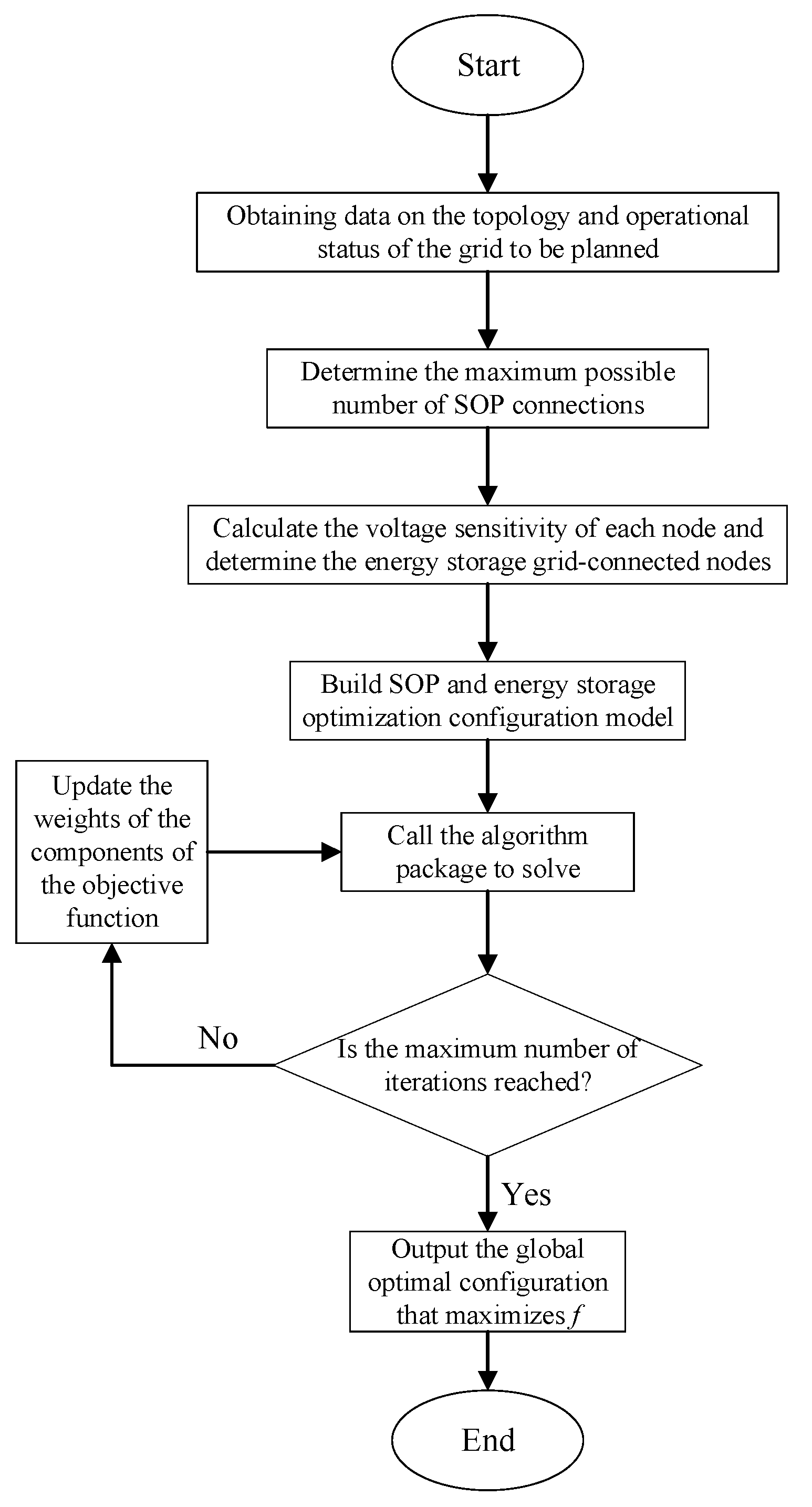
5. Solution Algorithm and Process

The flowchart of the SOP and energy storage optimization configuration method in a snowflake-shaped grid proposed in this article is presented in Figure 3. Firstly, data must be obtained on the topology and operational status of the planned power grid. Secondly, the maximum possible number of SOP-connected nodes between power grid stations is determined based on the snowflake-shaped grid structure. The energy storage connection nodes are then determined according to the calculation results of the voltage sensitivity of each node. Thirdly, an SOP and energy storage optimization configuration model must be constructed. Finally, call the algorithm package to solve and output the global optimal configuration that maximizes the objective function $f$ proposed in Section 4.

6. Example Analysis

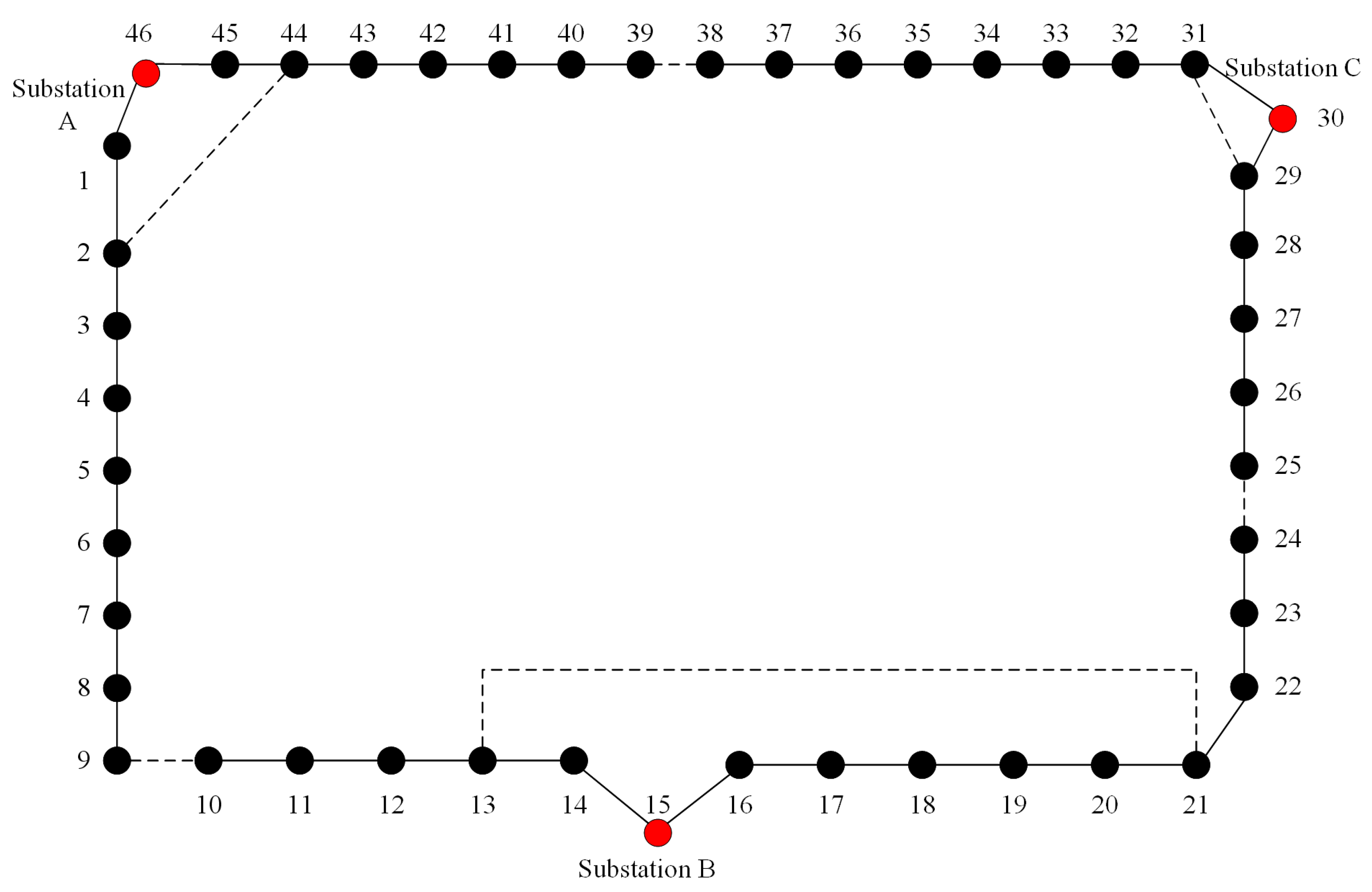
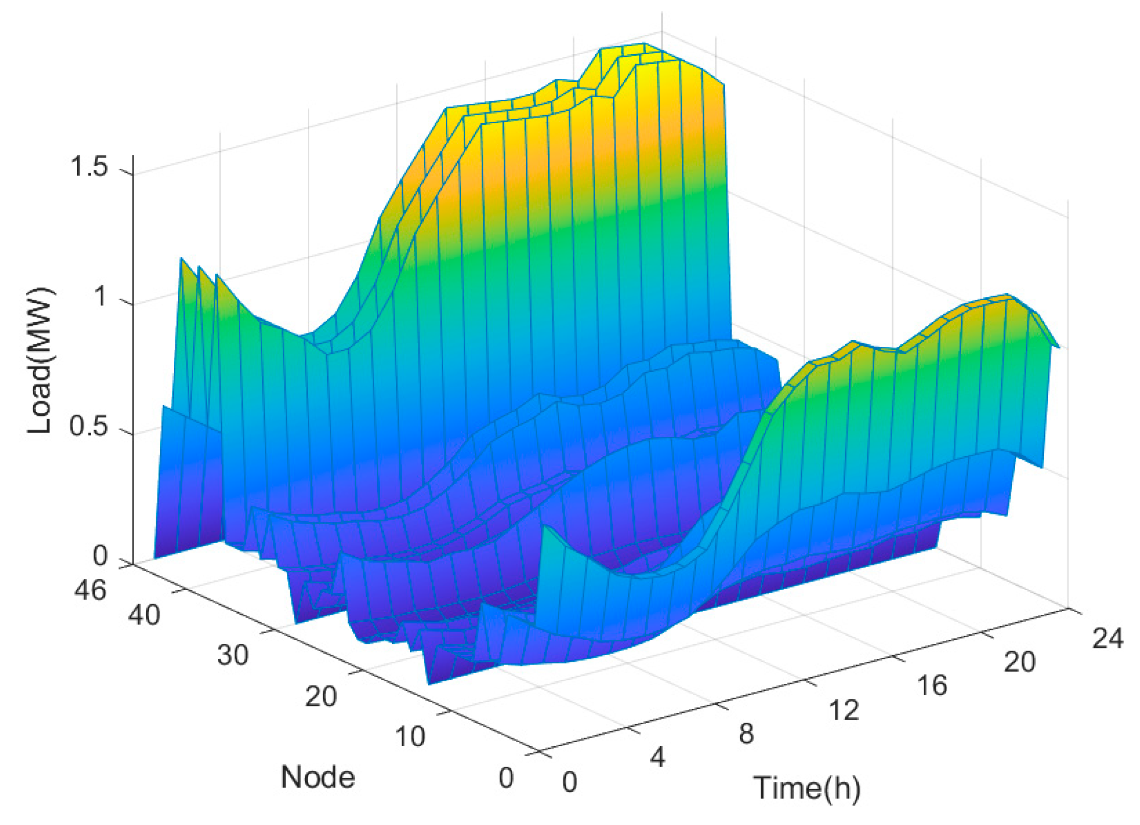
6.1. Example Introduction

This article employs a snowflake-shaped grid in Tianjin as an example to verify the effectiveness of the proposed SOP and energy storage optimization configuration method. The system structure is illustrated in Figure 4. The system operates at a rated voltage of 12.66 kV, and the typical daily load curve is illustrated in Figure 5. The branch impedance parameters are presented in

Table 1. Impedance parameters of grid branches of the snowflake-shaped grid.

Head Node	End Node	Resistance/Ω	Reactance/Ω
1	2	0.1633	0.1975
2	3	0.0294	0.0356
3	4	0.0189	0.0228
4	5	0.0132	0.0160
5	6	0.0244	0.0295
6	7	0.0170	0.0206
7	8	0.0212	0.0256
8	9	0.0256	0.0309
48	14	0.0679	0.1000
14	13	0.0980	0.1186
13	12	0.0253	0.0306
12	11	0.0300	0.0363
11	10	0.0186	0.0225
15	16	0.0679	0.1000
16	17	0.0566	0.0684
17	18	0.0211	0.0255
18	19	0.0072	0.0087
19	20	0.0083	0.0100
20	21	0.0124	0.0150
21	22	0.0253	0.0306
22	23	0.0300	0.0363
23	24	0.0186	0.0225
30	29	0.0699	0.1029
29	28	0.0083	0.0100
28	27	0.0232	0.0281
27	26	0.0202	0.0244
26	25	0.0142	0.0171
49	31	0.0439	0.0646
31	32	0.0566	0.0684
32	33	0.0189	0.0228
33	34	0.0132	0.0160
34	35	0.0244	0.0295
35	36	0.0166	0.0201
36	37	0.0212	0.0256
37	38	0.0260	0.0315
47	45	0.0637	0.0938
45	44	0.1616	0.1954
44	43	0.0535	0.0648
43	42	0.0142	0.0171
42	41	0.0202	0.0244
41	40	0.0277	0.0336
40	39	0.0083	0.0100
46	1	0.0511	0.0752

.

6.2. Analysis of SOP and Energy Storage Siting Results

In accordance with the distribution of inter-station connections in the snowflake-shaped grid illustrated in this example, the feasible installation locations for SOP are nodes 9–10, 13–21, 24–25, 29–31, 38–39, and 44–2. The maximum number of potential connections for SOP is six.

Calculate the voltage sensitivity of non-power nodes in the snowflake-shaped grid, as shown in Figure 6. It is recommended that nodes 9, 24, 38, 39, and 40 be designated as grid-connected nodes for energy storage.

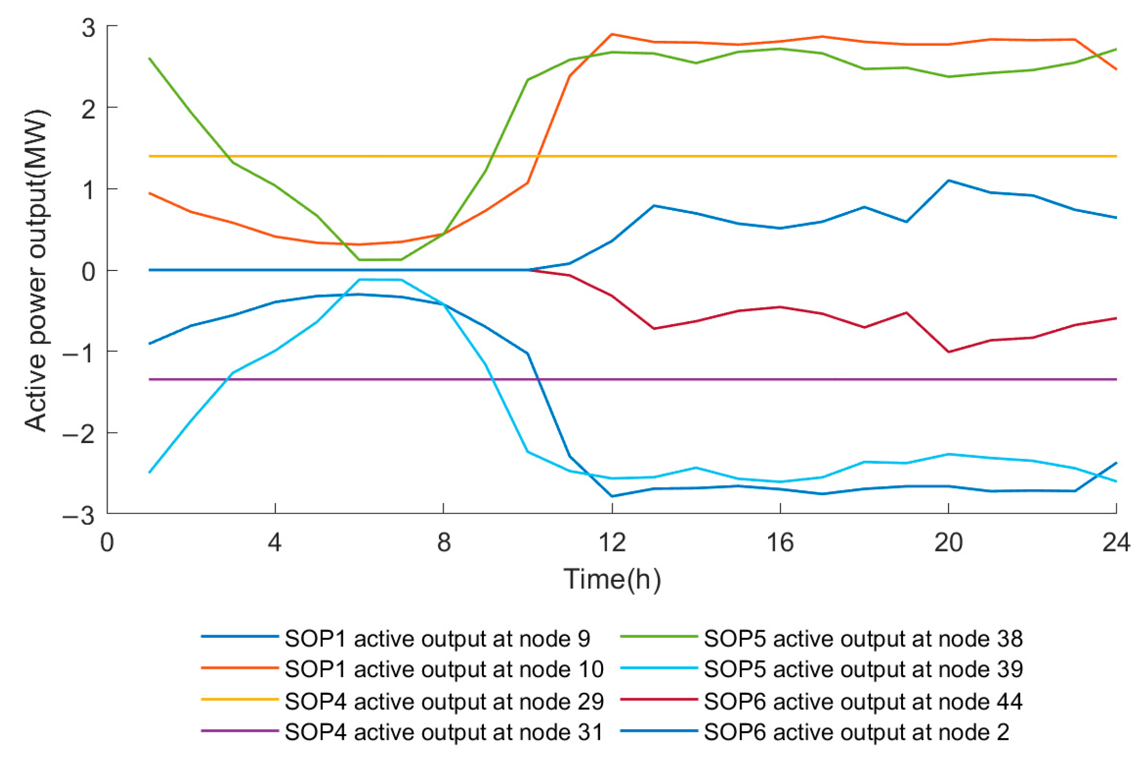
6.3. Analysis of SOP and Energy Storage Optimization Configuration Results

Once the SOP and energy storage site selection have been completed, the SOP and energy storage optimization configuration model should be constructed. The system operating parameters are as follows. The maximum allowable node voltage of the system is 1.05 p.u., the minimum allowable node voltage of the system is 0.95 p.u., and the maximum allowable branch current is 0.4 kA. The relevant parameters of the SOP are as follows. The service life of the SOP is 20 years. The investment cost per unit capacity of the SOP is CNY 1000/kVA. The cost coefficient of SOP operation and maintenance is 0.01. The loss coefficient of SOP is 0.02, and the discount rate of SOP is 0.08. The parameters related to energy storage are as follows. The maximum and minimum values of the energy storage state of charge are 0.9 and 0.1, respectively. The initial value of the energy storage state of charge is 0.5. The energy storage charging efficiency is 0.9, and the energy storage discharge efficiency is 0.9. The maximum energy storage charging and discharging rate is 0.2. The service life of energy storage is 20 years. The unit rated power cost of energy storage is CNY 1000/kW, and the unit capacity cost of energy storage is CNY 1200/kW. The operation and maintenance cost of the energy storage unit’s rated power is CNY 0.5/kW, and the discount rate of energy storage is 0.08.

In this paper, the SOP and energy storage optimization configuration models are solved through programming using the YALMIP optimization toolbox on the MATLAB R2023a platform and the IBM ILOG CPLEX 12.6 algorithmic package.

The SOP and energy storage access schemes can be classified into three distinct categories. Scheme 1 is designed to optimize the grid economy by configuring SOP and energy storage. Scheme 2, as proposed in this article, aims to balance the grid economy and load balancing by configuring SOP and energy storage. Finally, scheme 3 is intended to minimize load balancing through the configuration of SOP and energy storage. A comparison of the various SOP and energy storage configuration schemes is presented in

Table 2. Comparison of the results of different SOP and energy storage configuration scenarios.

Access Plan	Scheme 1	Scheme 2	Scheme 3
Node number for SOP access	9–10 29–31 38–39 44–2	9–10 29–31 38–39 44–2	9–10 13–21 24–25 29–31 38–39 44–2
SOP access capacity/kVA	2600 100 3000 2600	2900 1400 3000 2300	3000 1200 700 2300 3000 2300
Node number for energy storage access	39 40	40	38 40
Energy storage access capacity/kVA	2.52 1650	1670.02	770.09 1696.35
Annual investment cost of equipment/CNY 10,000	108.1	121.59	162.49
Annual operation and maintenance cost of equipment/CNY 10,000	8.32	9.62	12.52
Annual power loss cost of distribution network/CNY 10,000	80.24	113.63	203.23
Annual comprehensive cost/CNY 10,000	196.65	244.84	378.24
Load balancing	199.04	97.67	0

.

As illustrated in Table 2, scheme 2 incorporates both grid economy and load balancing considerations, in contrast with schemes 1 and 3. In terms of the annual comprehensive cost, the proposed scheme is 24.35% more expensive than scheme 1. Furthermore, it reduces load balancing by 50.93% in comparison to scheme 1.

In light of the aforementioned planning results, an analysis should be conducted to ascertain the extent to which SOP and energy storage optimize the operation of the snowflake-shaped grid when connected with the optimal configuration scheme. Figure 7 and Figure 8 illustrate the timing curves for the active and reactive power output of the SOP, respectively. Figure 9 illustrates the charging and discharging curves of the energy storage system at access node 40. As illustrated in the figure, SOP facilitates the transmission of the active power flow and provides reactive power compensation within the power grid, whereas energy storage optimizes the load distribution between feeders through the process of charging and discharging at different times.

7. Conclusions

This article puts forth a proposal for an SOP and energy storage optimization configuration method for the snowflake-shaped grid. Firstly, the location of the SOP is determined based on the characteristics of the interconnection nodes between snowflake websites, which are fully utilized in accordance with the snowflake-shaped grid structure. Secondly, the nodes that have a significant impact on the system voltage distribution are selected based on the voltage sensitivity analysis method, which is used to achieve the energy storage site selection. Subsequently, a multi-objective optimization configuration model for SOP and energy storage is established, taking into account the economic efficiency and load balancing of the power grid, in order to achieve a suitable capacity for SOP and energy storage. Finally, the method proposed in this paper is verified and analyzed using a snowflake-shaped grid in Tianjin as an example. The case analysis demonstrates that integrating SOP and energy storage can effectively enhance the power flow distribution between different feeders, balance the load, reinforce the reliability and stability of the power grid, and facilitate the integration of renewable energy in the future. In comparison with the plan that solely considers the economic aspects of the power grid, the methodology proposed in this article has the potential to reduce the degree of load balancing by 50.93% while simultaneously increasing the annual comprehensive cost by only 24.35%. The method proposed in this article can achieve the configuration of SOP and energy storage at the lowest possible economic cost while also optimizing the load balancing situation of the snowflake-shaped power grid to the greatest extent possible, and it has long-term economic sustainability. Further research could consider the high proportion of renewable energy integration with a view to further achieving economic and safe operation of the snowflake-shaped grid and fully tapping into its operational potential.

References

1. Zhuo, Z.Y.; Zhang, N. Key Technologies and Developing Challenges of Power System with High Proportion of Renewable Energy. Autom. Electr. Power Syst. 2021, 45, 171–191. [Google Scholar]
2. Zhang, Z.G.; Kang, C.Q. Challenges and Prospects for Constructing the New-type Power System Towards a Carbon Neutrality Future. Proc. CSEE 2022, 42, 2806–2819. [Google Scholar]
3. Wang, C.S.; Wang, S.Y. Economy and Reliability Analysis of Different Connection Modes in MV Distribution Systems. Autom. Electr. Power Syst. 2002, 26, 34–39. [Google Scholar]
4. Ruan, Q.T.; Xie, W. Research and Practice on the Upgrading for Diamond Distribution Network. Electr. Power 2020, 53, 1–7. [Google Scholar]
5. Wang, Z.; Duan, J.L. Exploration on Snow-shaped Grid Structure of Urban Medium Voltage Distribution Network. Proc. CSU-EPSA 2024, 36, 51–60. [Google Scholar]
6. Xiong, Z.Y.; Chen, T.H. Optimal Allocation of Soft Open Point in Active Distribution Network Based on Improved Sensitivity Analysis. Autom. Electr. Power Syst. 2021, 45, 129–137. [Google Scholar]
7. Ge, S.Y.; Zhou, C.X. Soft Open Point Planning for Active Distribution Network Considering Influence of Access Mode Between Feeder Loops and Reliability. Autom. Electr. Power Syst. 2021, 45, 120–128. [Google Scholar]
8. Wang, C.S.; Song, G.Y. Optimal Configuration of Soft Open Point for Active Distribution Network Considering the Characteristics of Distributed Generation. Proc. CSEE 2017, 37, 1889–1897. [Google Scholar]
9. Wang, H.Z.; Zhao, Q.Y. Improvement method of photovoltaic consumption capacity of AC/DC hybrid distribution network considering the time-of-use electricity price and SOP collaboration. Distrib. Util. 2023, 40, 1–9. [Google Scholar]
10. Guo, Y.; Wu, Q. MPC-based Coordinated Voltage Regulation for Distribution Networks with Distributed Generation and Energy Storage System. IEEE Trans. Sustain. Energy 2019, 10, 1731–1739. [Google Scholar] [CrossRef]
11. Chen, B.; Chen, C. Multi-time Step Service Restoration for Advanced Distribution Systems and Microgrids. IEEE Trans. Smart Grid 2018, 9, 6793–6805. [Google Scholar] [CrossRef]
12. Liu, X.; Aichhorn, A. Coordinated Control of Distributed Energy Storage System with Tap Changer Transformers for Voltage Rise Mitigation under High Photovoltaic Penetration. IEEE Trans. Smart Grid 2012, 3, 897–906. [Google Scholar] [CrossRef]
13. Bai, L.; Jiang, T. Distributed Energy Storage Planning in Soft Open Point Based Active Distribution Networks Incorporating Network Reconfiguration and DG Reactive Power Capability. Appl. Energ. 2018, 210, 1082–1091. [Google Scholar] [CrossRef]
14. Sun, C.B.; Li, J.R. Two-stage Optimization Method of Soft Open Point and Energy Storage System in Distribution Network Based on Interval Optimization. High Volt. Eng. 2021, 47, 45–54. [Google Scholar]
15. Li, J.; Liu, T.Q. Multi-criterion Integrated-sensitivity Voltage Stability Evaluation Index Based on Ideal Point Method. Electr. Power Autom. Equip. 2014, 34, 108–112. [Google Scholar]
16. Gao, B.; Morison, G.K. Towards the Development of A Systematic Approach for Voltage Stability Assessment of Largescale Power Systems. IEEE Trans. Power Syst. 1996, 11, 1314–1324. [Google Scholar] [CrossRef]
17. Song, G.Y. Operation and Planning Method of Soft Open Point for Multiple Scenarios in Active Distribution Network. Ph.D. Thesis, Tianjin University, Tianjin, China, 2017. [Google Scholar]
18. Li, P.; Ji, H. Coordinated Control Method of Voltage and Reactive Power for Active Distribution Networks Based on Soft Open Point. IEEE Trans. Sustain. Energy 2017, 4, 1430–1442. [Google Scholar] [CrossRef]
Figure 1. Schematic diagram of 10 kV snowflake-shaped grid structure. (a) Electrical schematic diagram. (b) Simplified schematic diagram.
Applsci 14 10503 g001aApplsci 14 10503 g001b
Figure 2. Grid wiring with 10 kV snowflake petals as the basic unit.
Applsci 14 10503 g002
Figure 3. SOP and energy storage configuration flowchart.
Applsci 14 10503 g003
Figure 4. Snowflake-shaped grid structure diagram.
Applsci 14 10503 g004
Figure 5. Typical daily load curve of the snowflake-shaped grid.
Applsci 14 10503 g005
Figure 6. Voltage sensitivity of non-power nodes of the snowflake-shaped grid.
Applsci 14 10503 g006
Figure 7. SOP active power output curve.
Applsci 14 10503 g007
Figure 8. SOP reactive power output curve.
Applsci 14 10503 g008
Figure 9. Energy storage charge/discharge curve at node 40.
Applsci 14 10503 g009