
Study on Quality Assessment Methods for Enhanced Resolution Graph-Based Reconstructed Images in 3D Capacitance Tomography


Abstract
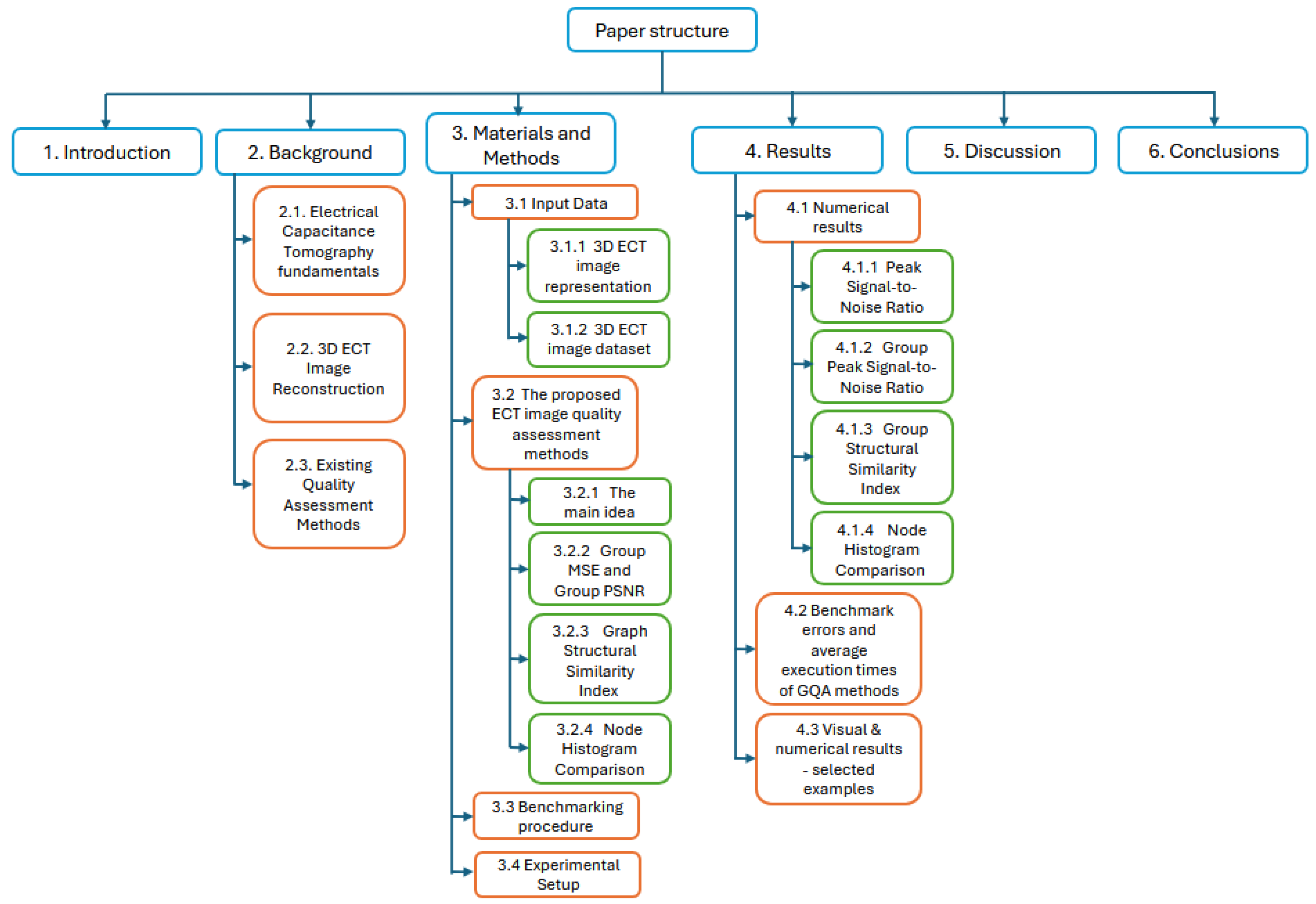
1. Introduction
2. Background
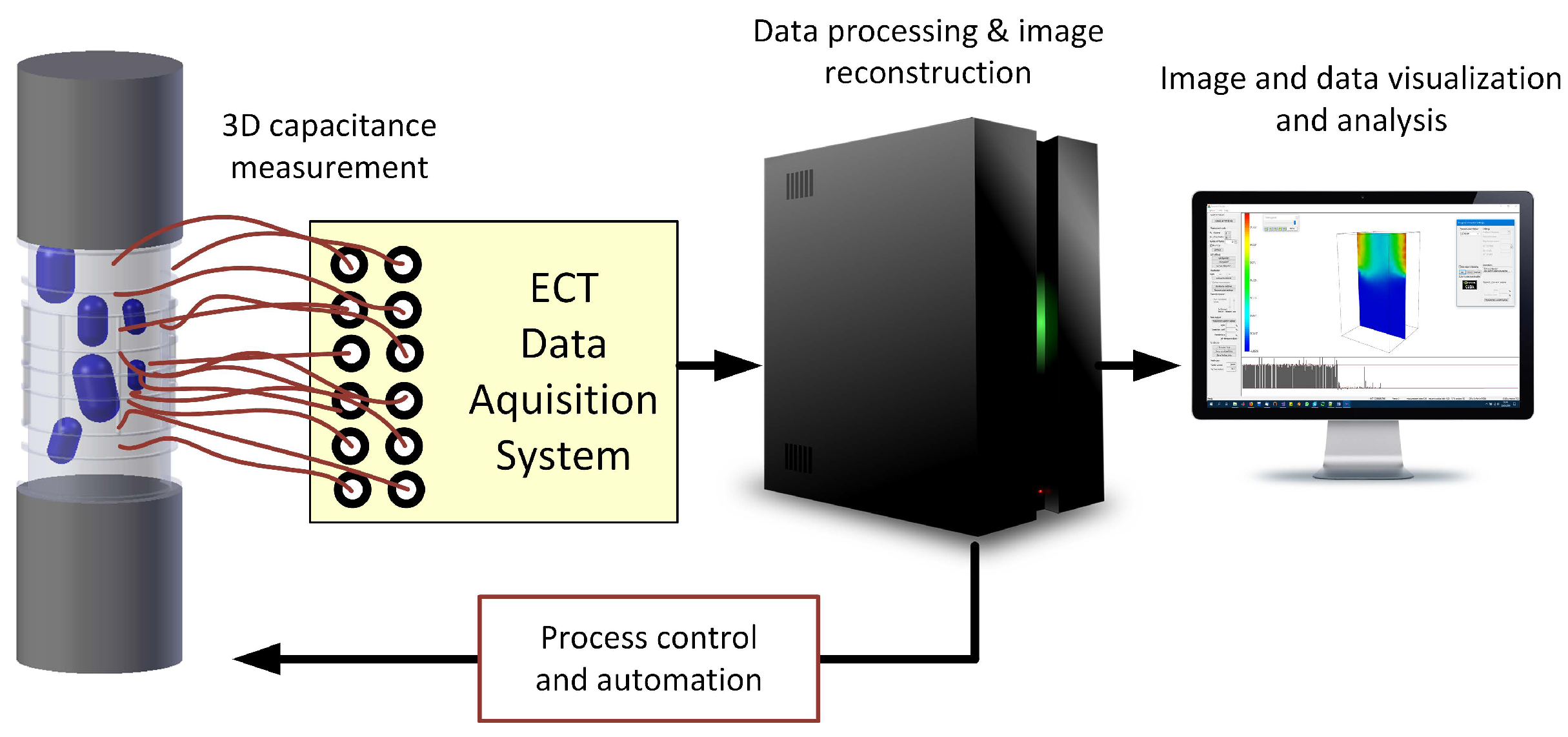
2.1. Electrical Capacitance Tomography Fundamentals
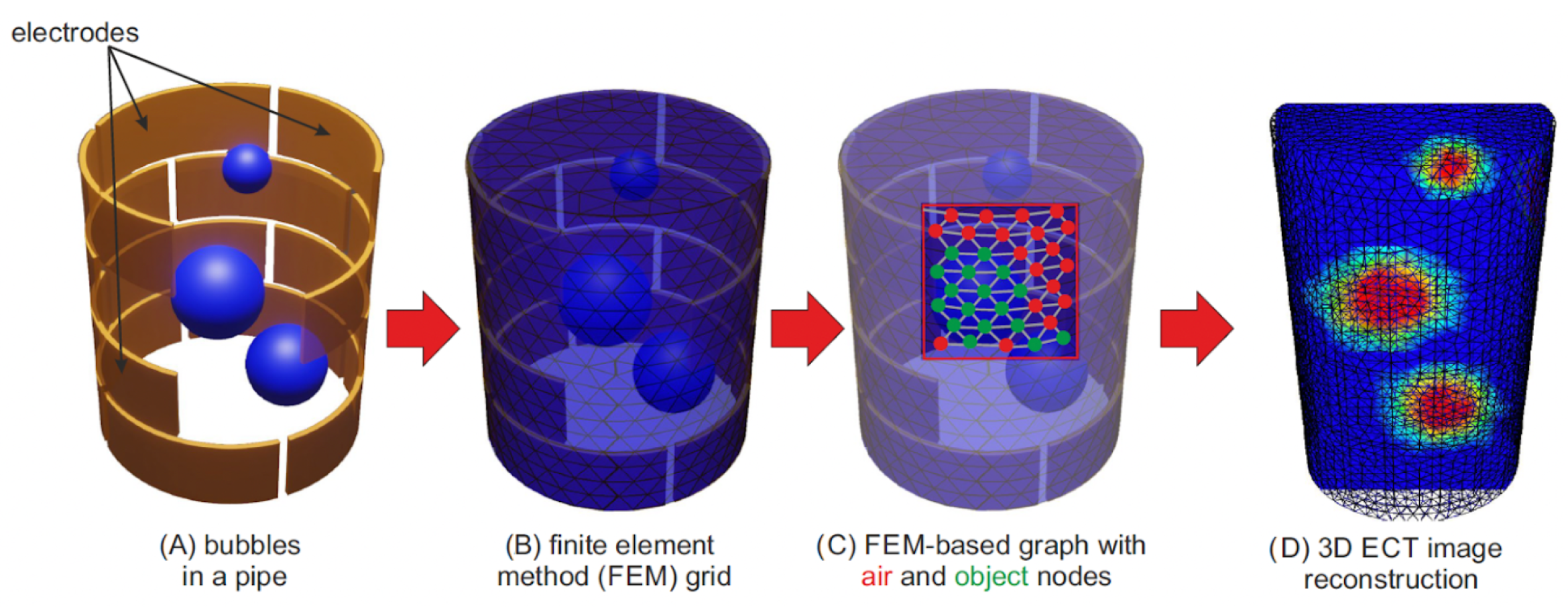
2.2. 3D ECT Image Reconstruction
2.3. Existing Quality Assessment Methods
3. Materials and Methods
3.1. Input Data
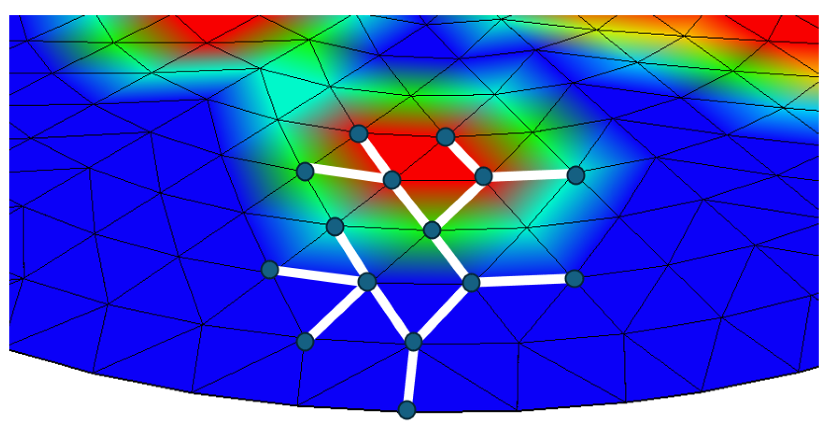
3.1.1. 3D ECT Image Representation
3.1.2. 3D ECT Image Dataset
3.2. The Proposed ECT Image Quality Assessment Methods
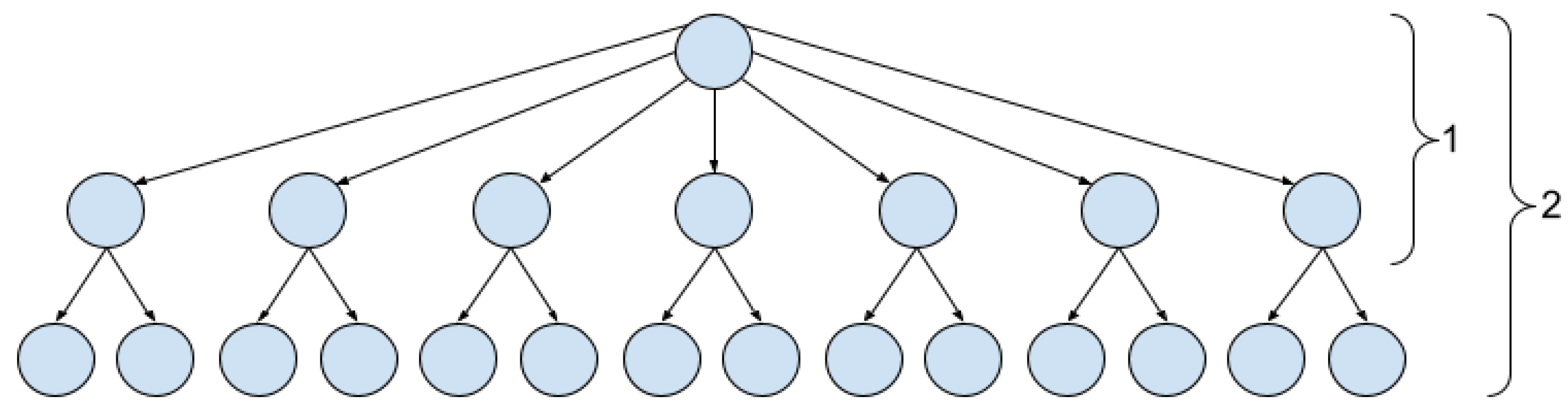
3.2.1. The Main Idea
3.2.2. Group MSE and Group PSNR
3.2.3. Graph Structural Similarity Index
3.2.4. Node Histogram Comparison
3.3. Benchmarking Procedure
- Error Rate: The percentage of phantom images where the LQ reconstruction received a higher similarity score than the HQ reconstruction.
- Execution Time: The average time the GQA method takes to calculate similarity measures for a single pair of images.
3.4. Experimental Setup
4. Results
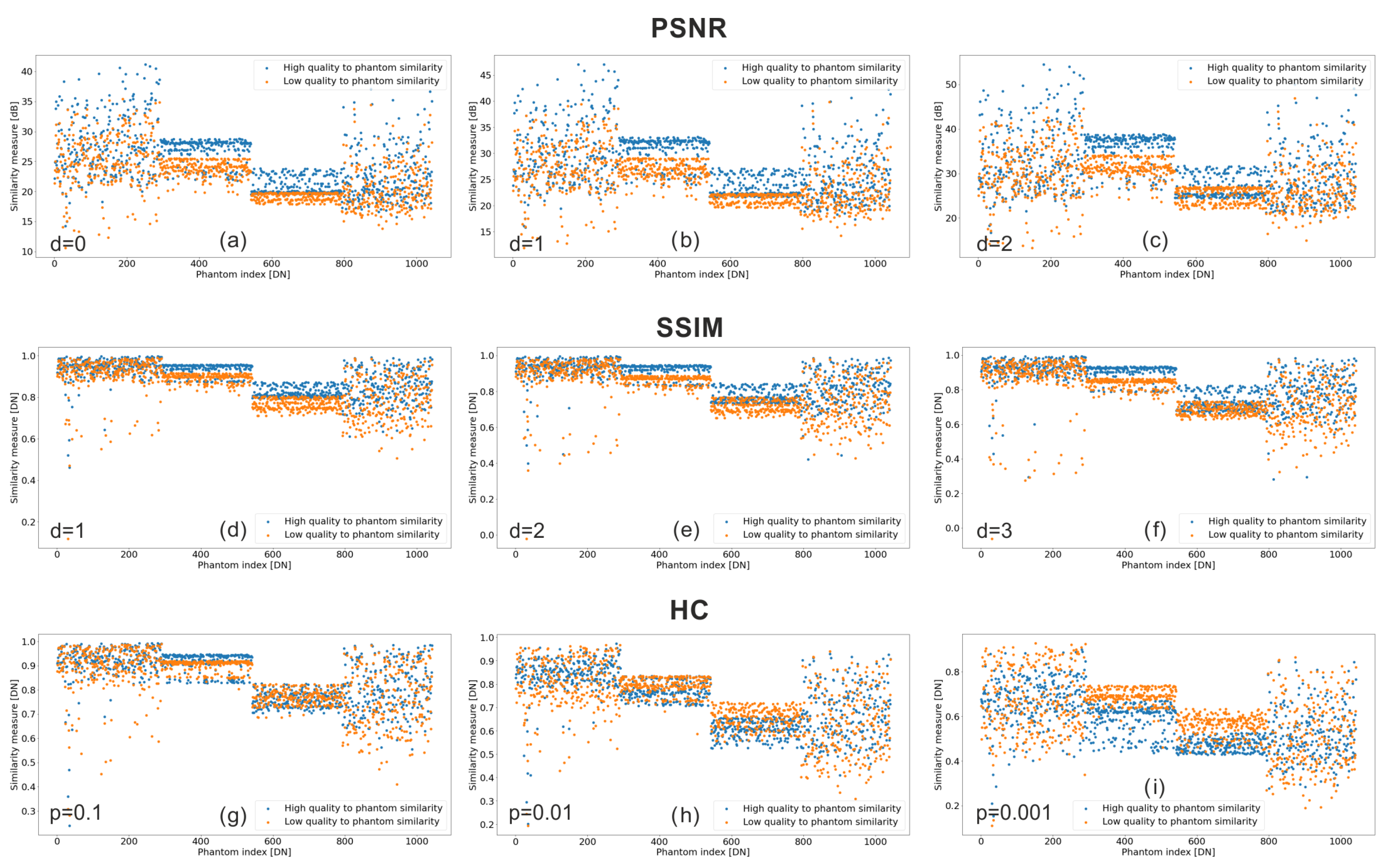
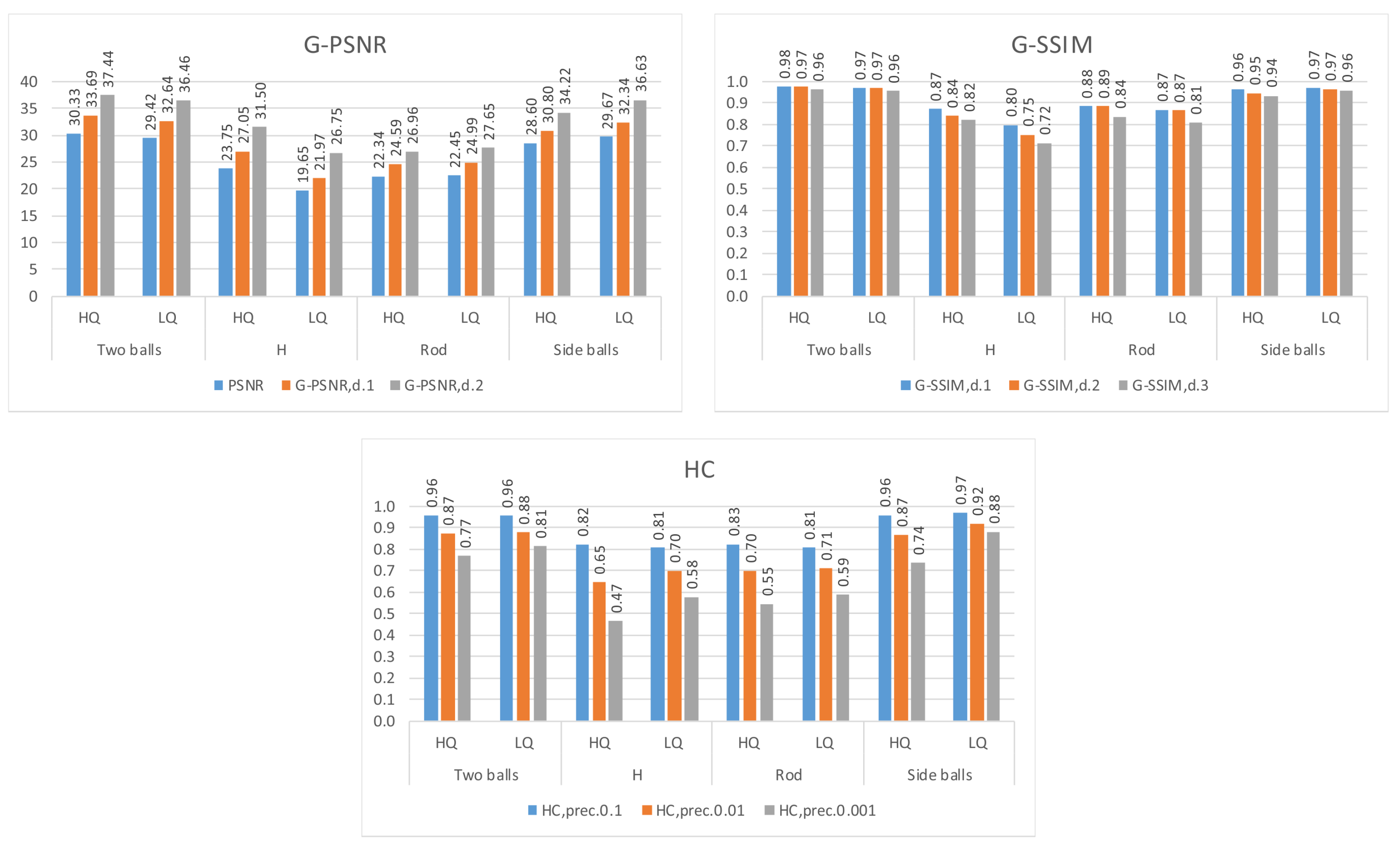
4.1. Numerical Results
- Peak Signal-to-Noise Ratio (PSNR)
- Group PSNR (depth 1 and 2)
- Group Structural Similarity Index Measure (G-SSIM) (depth 1, 2, and 3)
- Histogram Comparison (HC) (precision levels: 0.1, 0.01, and 0.001)
4.1.1. Peak Signal-to-Noise Ratio
- Period 1 → ball shapes: The initial 259 phantoms representing a ball shape showed a wide range of similarity values.
- Period 2 → H shapes: Phantoms 260–521, representing an H shape, demonstrated consistent similarity within each quality level, with clear differences between qualities.
- Period 3 → L shapes: Phantoms 522–783, representing an L shape, exhibited a tight clustering of Low-Quality values and a wider, evenly distributed spread for High-Quality values.
- Period 4 → rod shapes: Phantoms 784–end, representing a rod shape, showed a similar lack of consistency as Period 1, but with a narrower spread.
4.1.2. Group Peak Signal-to-Noise Ratio
4.1.3. Group Structural Similarity Index Measure
4.1.4. Node Histogram Comparison
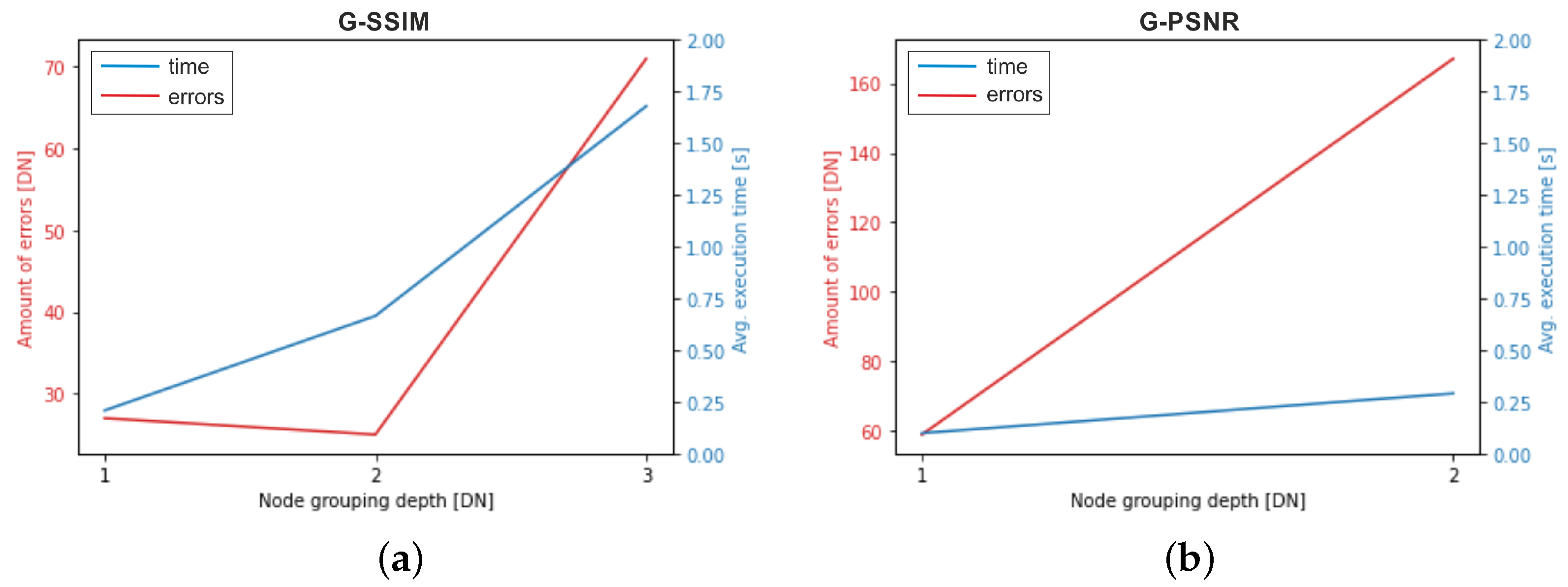
4.2. Benchmark Errors and Average Execution Times of GQA Methods
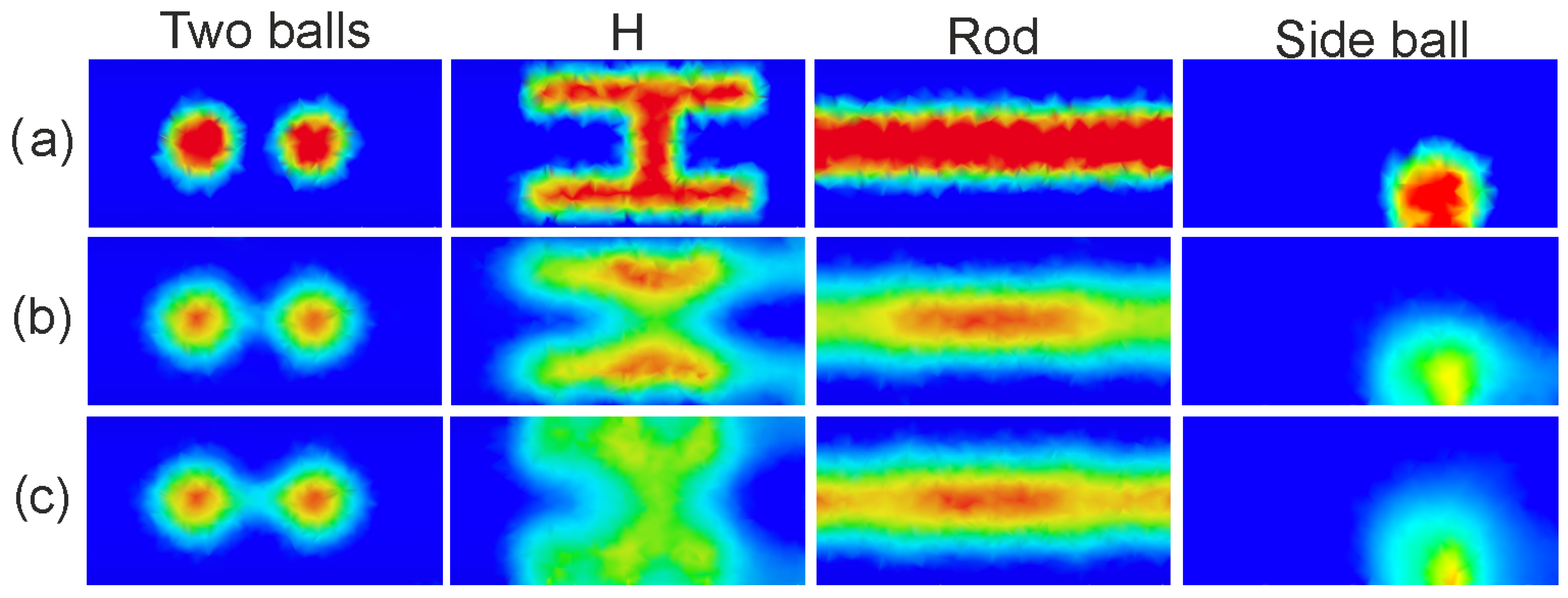
4.3. Visual and Numerical Results—Selected Examples
5. Discussion
6. Conclusions
Author Contributions
Funding
Institutional Review Board Statement
Informed Consent Statement
Data Availability Statement
Conflicts of Interest
References
- Yang, W.; Ren, Z.; Takei, M.; Yao, J. Medical applications of electrical tomography. In Proceedings of the 2018 IEEE International Conference on Imaging Systems and Techniques (IST), Krakow, Poland, 16–18 October 2018; pp. 1–6. [Google Scholar] [CrossRef]
- Huang, J.; Chen, F.; Wang, K.; Chen, S. Research on electrical capacitance tomography (ECT) detection of cerebral hemorrhage based on symmetrical cancellation method. Front. Phys. 2024, 12, 1392767. [Google Scholar] [CrossRef]
- Fabijańska, A.; Banasiak, R. Graph Convolutional Networks for Enhanced Resolution 3D Electrical Capacitance Tomography Image Reconstruction. Appl. Soft Comput. 2021, 110, 107608. [Google Scholar] [CrossRef]
- Wang, Z.; Bovik, A.C. Modern Image Quality Assessment; Morgan & Claypool: San Rafael, CA, USA, 2006. [Google Scholar]
- Dyakowski, T.; Jaworski, A. Non-Invasive Process Imaging – Principles and Applications of Industrial Process Tomography. Chem. Eng. Technol. 2003, 26, 697–706. [Google Scholar] [CrossRef]
- Yang, W.Q.; Peng, L. Image reconstruction algorithms for electrical capacitance tomography. Meas. Sci. Technol. 2002, 14, R1–R13. [Google Scholar] [CrossRef]
- Wajman, R.; Banasiak, R.; Mazurkiewicz, L.; Dyakowski, T.; Sankowski, D. Spatial imaging with 3D capacitance measurements. Meas. Sci. Technol. 2006, 17, 2113–2118. [Google Scholar] [CrossRef]
- Warsito, W.; Fan, L.S. Development of three-dimensional electrical capacitance tomography. In Proceedings of the 3rd World Congress on Industrial Process Tomography, Banff, AB, Canada, 2–5 September 2003; pp. 391–396. [Google Scholar]
- Banasiak, R.; Wajman, R.; Sankowski, D.; Soleimani, M. Three-dimensional nonlinear inversion of electrical capacitance tomography data using a complete sensor model. Prog. Electromagn. Res. 2010, 100, 219–234. [Google Scholar] [CrossRef]
- Soleimani, M.; Lionheart, W. Nonlinear Image Reconstruction for Electrical Capacitance Tomography Using Experimental Data. Meas. Sci. Technol. 2005, 16, 1987. [Google Scholar] [CrossRef]
- Jaworski, A.; Dyakowski, T. Application of Electrical Capacitance Tomography for Measurement of Gas-Solids Flow Characteristics in a Pneumatic Conveying System. Meas. Sci. Technol. 2001, 12, 1109. [Google Scholar] [CrossRef]
- Majchrowicz, M.; Kapusta, P.; Jackowska-Strumillo, L.; Banasiak, R.; Sankowski, D. Multi-GPU, Multi-Node Algorithms for Acceleration of Image Reconstruction in 3D Electrical Capacitance Tomography in Heterogeneous Distributed System. Sensors 2020, 20, 391. [Google Scholar] [CrossRef]
- Tapson, J. Neural networks and stochastic search methods applied to industrial capacitive tomography. Control Eng. Pract. 1999, 7, 117–121. [Google Scholar] [CrossRef]
- Watzenig, D.; Fox, C. A review of statistical modelling and inference for electrical capacitance tomography. Meas. Sci. Technol. 2009, 20, 052002. [Google Scholar] [CrossRef]
- Chen, D.Y.; Chen, Y.; Wang, L.L.; Yu, X.Y. A novel Gauss-Newton image reconstruction algorithm for Electrical Capacitance Tomography System. Tien Tzu Hsueh Pao/Acta Electron. Sin. 2009, 37, 739–743. [Google Scholar]
- Zheng, J.; Peng, L. An Autoencoder Based Image Reconstruction for Electrical Capacitance Tomography. IEEE Sens. J. 2018, 18, 5464–5474. [Google Scholar] [CrossRef]
- Lei, J.; Liu, Q.; Wang, X. Deep Learning-Based Inversion Method for Imaging Problems in Electrical Capacitance Tomography. IEEE Trans. Instrum. Meas. 2018, 67, 2107–2118. [Google Scholar] [CrossRef]
- Zheng, J.; Ma, H.; Peng, L. A CNN-Based Image Reconstruction for Electrical Capacitance Tomography. In Proceedings of the 2019 IEEE International Conference on Imaging Systems and Techniques (IST), Abu Dhabi, United Arab Emirates, 9–10 December 2019; pp. 1–6. [Google Scholar] [CrossRef]
- Wang, L.; Liu, X.; Chen, D.; Yang, H.; Wang, C. ECT Image Reconstruction Algorithm Based on Multiscale Dual-Channel Convolutional Neural Network. Complexity 2020, 2020, 4918058. [Google Scholar] [CrossRef]
- Cao, Z.; Xu, L.; Fan, W.; Wang, H. Electrical capacitance tomography with a non-circular sensor using the dbar method. Meas. Sci. Technol. 2009, 21, 015502. [Google Scholar] [CrossRef]
- Kulisz, M.; Kłosowski, G.; Rymarczyk, T.; Hoła, A.; Niderla, K.; Sikora, J. The use of the multi-sequential LSTM in electrical tomography for masonry wall moisture detection. Measurement 2024, 234, 114860. [Google Scholar] [CrossRef]
- Kulisz, M.; Kłosowski, G.; Rymarczyk, T.; Słoniec, J.; Gauda, K.; Cwynar, W. Optimizing the Neural Network Loss Function in Electrical Tomography to Increase Energy Efficiency in Industrial Reactors. Energies 2024, 17, 681. [Google Scholar] [CrossRef]
- Guo, Q.; Li, X.; Hou, B.; Mariethoz, G.; Ye, M.; Yang, W.; Liu, Z. A Novel Image Reconstruction Strategy for ECT: Combining Two Algorithms With a Graph Cut Method. IEEE Trans. Instrum. Meas. 2020, 69, 804–814. [Google Scholar] [CrossRef]
- Deabes, W.; Abdel-Hakim, A.E.; Bouazza, K.E.; Althobaiti, H. Adversarial Resolution Enhancement for Electrical Capacitance Tomography Image Reconstruction. Sensors 2022, 22, 3142. [Google Scholar] [CrossRef]
- Wang, F.; Marashdeh, Q.; Fan, L.S.; Warsito, W. Electrical Capacitance Volume Tomography: Design and Applications. Sensors 2010, 10, 1890–1917. [Google Scholar] [CrossRef] [PubMed]
- Wang, Z.; Bovik, A.; Sheikh, H.; Simoncelli, E. Image quality assessment: From error visibility to structural similarity. IEEE Trans. Image Process. 2004, 13, 600–612. [Google Scholar] [CrossRef] [PubMed]


| Shape | Number | Random Parameters |
|---|---|---|
| multiple balls | 259 | number (2–5), radius, position |
| H-shape | 262 | size, position, orientation |
| L-shape | 262 | size, position, orientation |
| rod | 259 | number (1–5), diameter, length, position |
| GQA Method | Amount of Errors | Average Execution Time [s] |
|---|---|---|
| G-SSIM, depth 2 | 25 | 0.6648 |
| G-SSIM, depth 1 | 27 | 0.2075 |
| PSNR | 43 | 0.0034 |
| G-PSNR, depth 1 | 59 | 0.0977 |
| G-SSIM, depth 3 | 71 | 1.6794 |
| G-PSNR, depth 2 | 167 | 0.2899 |
| HC, prec. 0.1 | 274 | 0.0585 |
| HC, prec. 0.01 | 590 | 0.0594 |
| HC, prec. 0.001 | 736 | 0.0664 |
Disclaimer/Publisher’s Note: The statements, opinions and data contained in all publications are solely those of the individual author(s) and contributor(s) and not of MDPI and/or the editor(s). MDPI and/or the editor(s) disclaim responsibility for any injury to people or property resulting from any ideas, methods, instructions or products referred to in the content. |
© 2024 by the authors. Licensee MDPI, Basel, Switzerland. This article is an open access article distributed under the terms and conditions of the Creative Commons Attribution (CC BY) license (https://creativecommons.org/licenses/by/4.0/).
Share and Cite
Banasiak, R.; Bujnowicz, M.; Fabijańska, A. Study on Quality Assessment Methods for Enhanced Resolution Graph-Based Reconstructed Images in 3D Capacitance Tomography. Appl. Sci. 2024, 14, 10222. https://doi.org/10.3390/app142210222
Banasiak R, Bujnowicz M, Fabijańska A. Study on Quality Assessment Methods for Enhanced Resolution Graph-Based Reconstructed Images in 3D Capacitance Tomography. Applied Sciences. 2024; 14(22):10222. https://doi.org/10.3390/app142210222
Chicago/Turabian StyleBanasiak, Robert, Mateusz Bujnowicz, and Anna Fabijańska. 2024. "Study on Quality Assessment Methods for Enhanced Resolution Graph-Based Reconstructed Images in 3D Capacitance Tomography" Applied Sciences 14, no. 22: 10222. https://doi.org/10.3390/app142210222
APA StyleBanasiak, R., Bujnowicz, M., & Fabijańska, A. (2024). Study on Quality Assessment Methods for Enhanced Resolution Graph-Based Reconstructed Images in 3D Capacitance Tomography. Applied Sciences, 14(22), 10222. https://doi.org/10.3390/app142210222