Article

A Tuning Method for Speed Tracking Controller Parameters of Autonomous Vehicles

School of Mechanical Engineering, Shenyang University of Technology, Shenyang 110870, China
*
Author to whom correspondence should be addressed.
Appl. Sci. 2024, 14(22), 10209; https://doi.org/10.3390/app142210209
Submission received: 7 October 2024 / Revised: 30 October 2024 / Accepted: 1 November 2024 / Published: 7 November 2024
(This article belongs to the Special Issue Intelligent Robot: Design, Control and Optimization)

Abstract

:
Autonomous driving technology, as a key component of intelligent transportation systems, has gained considerable attention in recent years. While significant progress has been made in areas such as path planning, obstacle detection, and navigation, relatively less focus has been placed on vehicle speed control, which plays a critical role in ensuring safe and efficient operation, especially in complex and dynamic road environments. This paper addresses the challenge of speed tracking by proposing a genetic algorithm-based optimization method for PID controller parameters. Traditional PID controllers often struggle with maintaining accuracy and response time in highly variable conditions, but by optimizing these parameters through the genetic algorithm, substantial improvements in speed control precision and adaptability can be achieved, enhancing the vehicle’s ability to navigate real-world driving scenarios with greater stability. The experimental results clearly indicate that the autonomous vehicle, after PID parameter optimization using a genetic algorithm, demonstrated the following speed tracking errors: when the road surface adhesion coefficient was 0.5, the maximum speed tracking error was 0.22, the average value was 0.063, and the standard deviation was 0.124; when the adhesion coefficient was 0.6, the maximum speed tracking error was 0.180, the average value was 0.056, and the standard deviation was 0.099; when the adhesion coefficient was 0.8, the maximum speed tracking error was 0.179, the average value was 0.056, and the standard deviation was 0.098. This method significantly improved the controller’s performance in maintaining the desired speed, even under challenging conditions. These findings highlight the potential of genetic algorithms in supporting the future development of autonomous driving technology, ensuring its successful integration into intelligent transportation systems.

1. Introduction

With the rapid development of artificial intelligence and automation technologies, autonomous vehicles have become a key research focus in the field of intelligent transportation. These vehicles are expected to transform our perception of mobility by providing safer, more efficient, and more convenient transportation options. Among the numerous challenges faced by autonomous driving, vehicle motion control, particularly speed control, plays a crucial role. Accurate speed control is essential for ensuring smooth driving, enhancing safety, and improving passenger comfort. However, despite significant advancements in areas such as path planning and obstacle detection [1,2,3,4,5,6,7,8], research specifically focused on speed tracking control remains relatively limited.
Speed control is not only crucial for responding to constantly changing road conditions but also directly affects energy consumption and operational stability. In fact, precise speed control is one of the key challenges in the development of autonomous driving technology. Traditional PID (proportional–integral–derivative) controllers are widely used in industrial control systems due to their simplicity and effectiveness [9,10,11,12,13]. However, the performance of PID controllers heavily depends on the correct tuning of parameters, which is often carried out manually and based on empirical methods [14,15,16,17,18,19,20]. In complex and dynamic driving environments, this reliance on experience can prevent the controller from achieving optimal performance.
In recent years, although numerous studies have introduced intelligent optimization algorithms into the design of controller parameters within industrial control systems [20,21,22,23,24,25,26], to date, no research has specifically applied optimization algorithms to determine vehicle speed controller parameters. Based on this gap, this study proposes a genetic algorithm-based PID parameter optimization method tailored for speed control in autonomous vehicles, applying it within the field of intelligent driving. This method addresses the limitations of traditional manual tuning by implementing an automated optimization process that can adapt to changing road conditions. Experimental results indicate that this approach significantly improves speed control accuracy, reduces error, and enhances system responsiveness. These findings demonstrate that our method provides an effective solution for real-world autonomous driving applications, offering greater stability, efficiency, and adaptability in complex driving environments.
The second part of this study introduces the construction of the longitudinal PID controller for the vehicle, the third part presents PID controller parameter optimization, the fourth part provides the simulation results and discussion, and the fifth part contains the conclusion.

2. Construction of Longitudinal PID Controller for a Vehicle

The longitudinal motion model of an autonomous vehicle, which refers to the movement in the forward and backward directions, is crucial for describing the vehicle’s dynamic behavior during various driving conditions such as acceleration, deceleration, and constant-speed cruising. This model serves as a foundation for controlling and tracking the vehicle’s speed, enabling the vehicle to respond appropriately to the environment and driver commands.
The model is based on Newton’s second law of motion, which states that the acceleration of an object is determined by the net forces acting upon it. In the context of vehicle dynamics, the model considers the balance of various forces, including driving force, resistance from the air, rolling friction from the tires, and braking forces. By analyzing these forces, the model predicts changes in the vehicle’s acceleration, speed, and displacement over time. This makes the longitudinal motion model essential for implementing precise speed control in autonomous driving systems, ensuring the vehicle can adjust smoothly and safely during different driving scenarios.

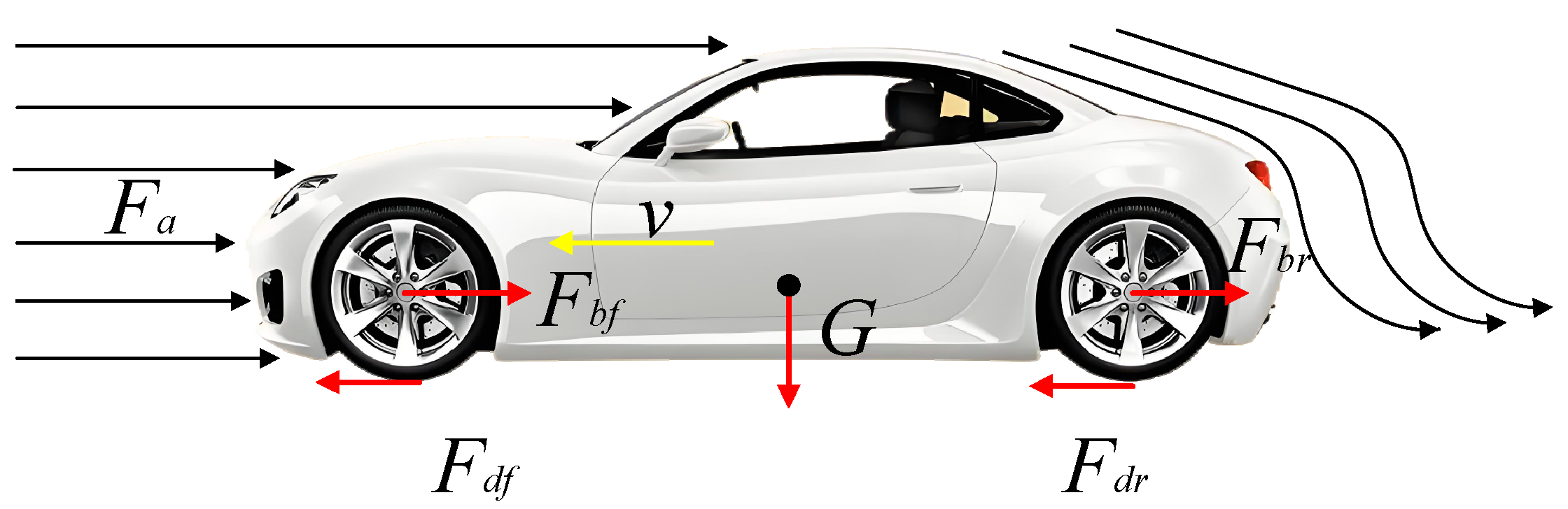
2.1. Longitudinal Dynamics Modeling of the Vehicle

This study only considers the driving of the autonomous vehicle on a flat road surface; thus, the gradient resistance is zero. The force analysis diagram of the longitudinal model of the autonomous vehicle is shown in Figure 1.
In longitudinal motion, the vehicle is primarily influenced by the following four forces:
(1)
Driving Force F d : The driving force is provided by the engine or motor and transmitted to the wheels through the drivetrain.
F d = F d f + F d r
F d is the driving force on the front wheels, and F d r is the driving force on the rear wheels.
F d μ F i
where μ is the road adhesion coefficient, and F i is the vertical load on the wheels.
(2)
Aerodynamic Drag F a : This is proportional to the square of the vehicle’s speed, and typically expressed as
F a = 1 2 ρ C d A d v 2
where ρ is the air density, C d is the drag coefficient, and A d is the frontal area of the vehicle.
(3)
Rolling Resistance F r : The friction force between the tires and the road, expressed as
F r = C r m g
where C r is the rolling resistance coefficient and m is the mass of the vehicle.
(4)
Braking Force F b : Generated by the braking system, controlling the deceleration of the vehicle.
F b = F b f + F b r
F b f is the front-wheel braking force, and F b r is the rear-wheel braking force.
F b μ F i
where μ is the road adhesion coefficient, and F i is the vertical load on the wheels.
The longitudinal dynamics model of the autonomous vehicle is expressed as
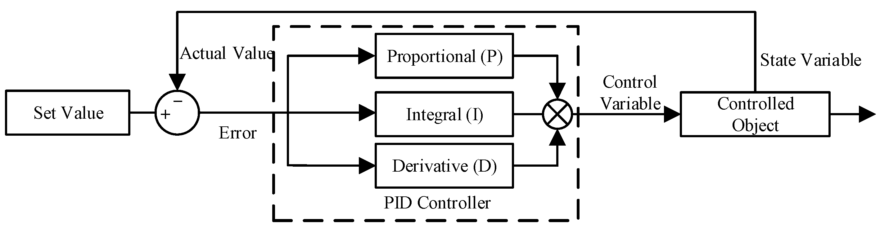
m v = min F d , μ F i 1 2 ρ C d A d v 2 + C r m g min μ F i , F b .

2.2. PID Control

The PID controller is a control algorithm that is widely used in automatic control systems, adjusting the output of the controlled object to ensure that the system reaches the desired target value. The core concept of the PID controller is feedback control based on the control error (i.e., the difference between the setpoint and the actual value), ensuring both fast response speed and high accuracy of the system. This algorithm is recognized for its simplicity and effectiveness, making it suitable for a wide range of industrial processes and control scenarios.
PID controllers can be classified into multiple types based on different criteria. According to the implementation method, they can be divided into analog and digital PID controllers: analog PID controllers rely on electronic circuits, while digital PID controllers use discrete computations and digital signal processing. Based on the form of the control algorithm, they can be categorized as positional or incremental controllers: positional controllers calculate a target position based on the current error, while incremental controllers make adjustments based on changes in the error. From the structural perspective, there are parallel and series controllers: parallel controllers compute contributions independently, while series controllers handle them sequentially. In terms of parameter adjustment methods, they can be classified into fixed-parameter and adaptive PID controllers: fixed-parameter controllers use constant values, while adaptive controllers adjust parameters in response to system changes. Depending on the number of control loops, they can be classified as single-loop or multi-loop controllers, where multi-loop controllers manage multiple variables simultaneously. Based on application fields, PID controllers can be divided into general purpose and specialized PID controllers, tailored to meet the needs of specific industries. Regarding the implementation platform, PID controllers can be classified as hardware- or software-based controllers, where hardware controllers are implemented via physical devices and software controllers through computer programs. Lastly, based on control action, there are P (proportional), PI (proportional–integral), PD (proportional–derivative), and PID (proportional–integral–derivative) controllers. These classifications help users select the most suitable PID controller according to specific control requirements, aiming to achieve optimal performance.
The PID controller used in this study is composed of three parts: proportional (P), integral (I), and derivative (D), each contributing differently to the controller’s output. The proportional component provides a basic response by reacting instantly to the error signal; the integral component works to eliminate the steady-state error, ensuring that the system eventually reaches the target value; and the derivative component predicts the change in the error trend, enhancing the dynamic response and minimizing overshoot. The basic principle of the PID controller is illustrated in Figure 2, which visually explains how each part cooperates to improve the system’s control performance.
In this study, a PID control method is used to manage the longitudinal speed tracking of a vehicle. Proportional control (P) adjusts based on the current error value (i.e., the difference between the target speed and the actual speed). The output of the proportional controller is directly proportional to the error, meaning that the larger the error, the stronger the controller’s response, which enables a quick reaction to speed deviations. The control rule is as follows:
P = k p e t + k i e t d t + k d d e t d t
where k p is the proportional coefficient, and e t represents the speed error (the difference between the target speed and the actual speed).
The advantage of proportional control is its ability to respond quickly to speed changes. However, using proportional control alone may lead to steady-state errors, meaning that the vehicle’s speed may never fully reach the target value.
To eliminate this steady-state error, integral control (I) is introduced in this study, which adjusts the system based on the accumulated error over time. When the vehicle deviates from the target speed for an extended period, the integral controller gradually increases the output until the error is eliminated. The control rule is
I = k i e t d t
where k i is the integral coefficient, and e t d t represents the accumulated error.
Additionally, to reduce overshoot and improve system stability, derivative control (D) is used in this study. Derivative control adjusts the system based on the rate of change in the error, predicting the trend of the error to mitigate excessive fluctuations in vehicle speed. The control rule is
D = k d d e t d t
where k d is the derivative coefficient, and k d d e t d t is the rate of change in the error.
By combining the proportional, integral, and derivative components, the PID controller achieves fast, accurate, and stable speed tracking control. This method ensures that the vehicle’s longitudinal speed follows the target speed as quickly as possible while maintaining stability. The overall control formula is
u t = k p e t + k i e t d t + k d d e t d t
The PID controller’s advantage lies in the combination of proportional control’s fast response, integral control’s ability to eliminate steady-state errors, and derivative control’s overshoot suppression, making longitudinal speed control smoother and more precise.

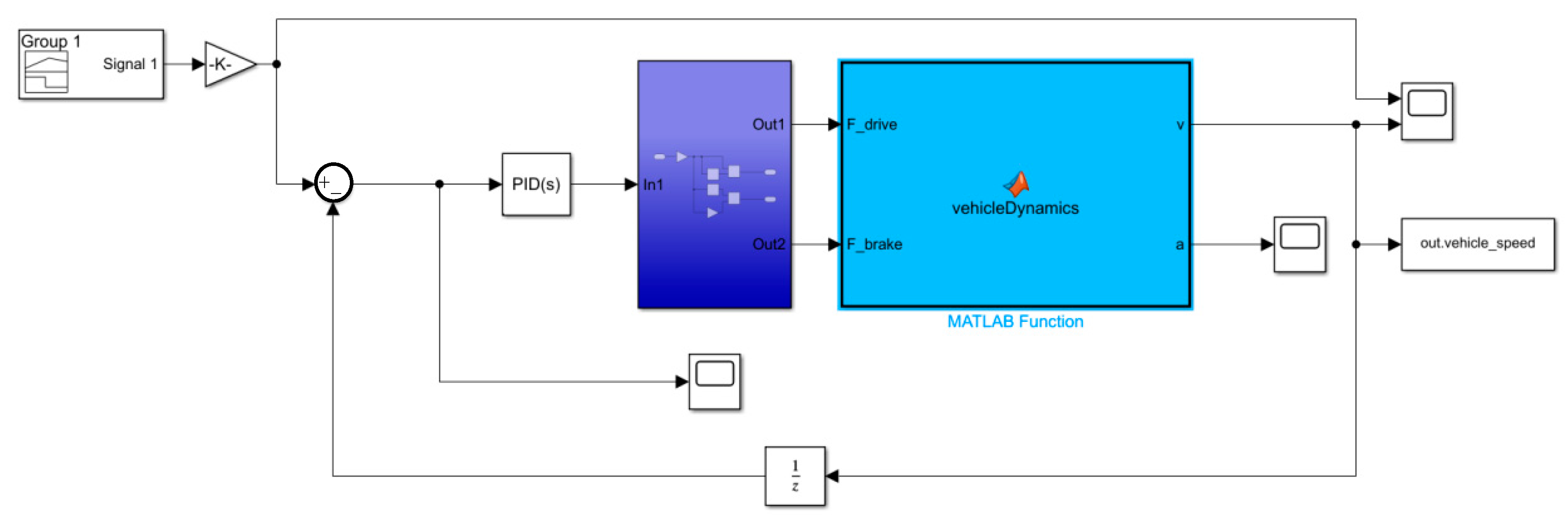
2.3. PID Controller Construction

In this study, MATLAB/Simulink(2019b) is used to construct the PID controller. The model diagram of the PID controller is shown in Figure 3.
In this study, the input to the PID controller is the difference between the target speed and the actual speed, and the output is used to adjust the driving force to regulate the vehicle speed, making it approach the target speed and achieve precise control.

3. PID Controller Parameter Optimization

The performance of the PID controller depends on the tuning of three parameters: k p , k i , and k d . However, these parameters are often set based on experience, which makes it difficult for the controller to achieve optimal performance. This study uses an optimization algorithm to automatically adjust the PID parameters, improving control accuracy, reducing overshoot and oscillation, and speeding up system response. Compared to manual tuning, optimization algorithms are better equipped to handle complex environments and uncertainties, ensuring the controller operates stably under variable road conditions. This approach reduces reliance on experience and finds the global optimal solution, significantly enhancing system performance.
Using a genetic algorithm to optimize PID parameters offers notable advantages. Its global search capability avoids local optima and finds better parameter combinations. Genetic algorithms are well suited for complex, nonlinear, multivariable problems and remain effective even when dealing with discontinuous or noisy systems. They also exhibit strong robustness, being less sensitive to initial parameters, thus ensuring the stability of PID control. The parallel processing ability makes the optimization process more efficient, quickly finding the optimal parameters.

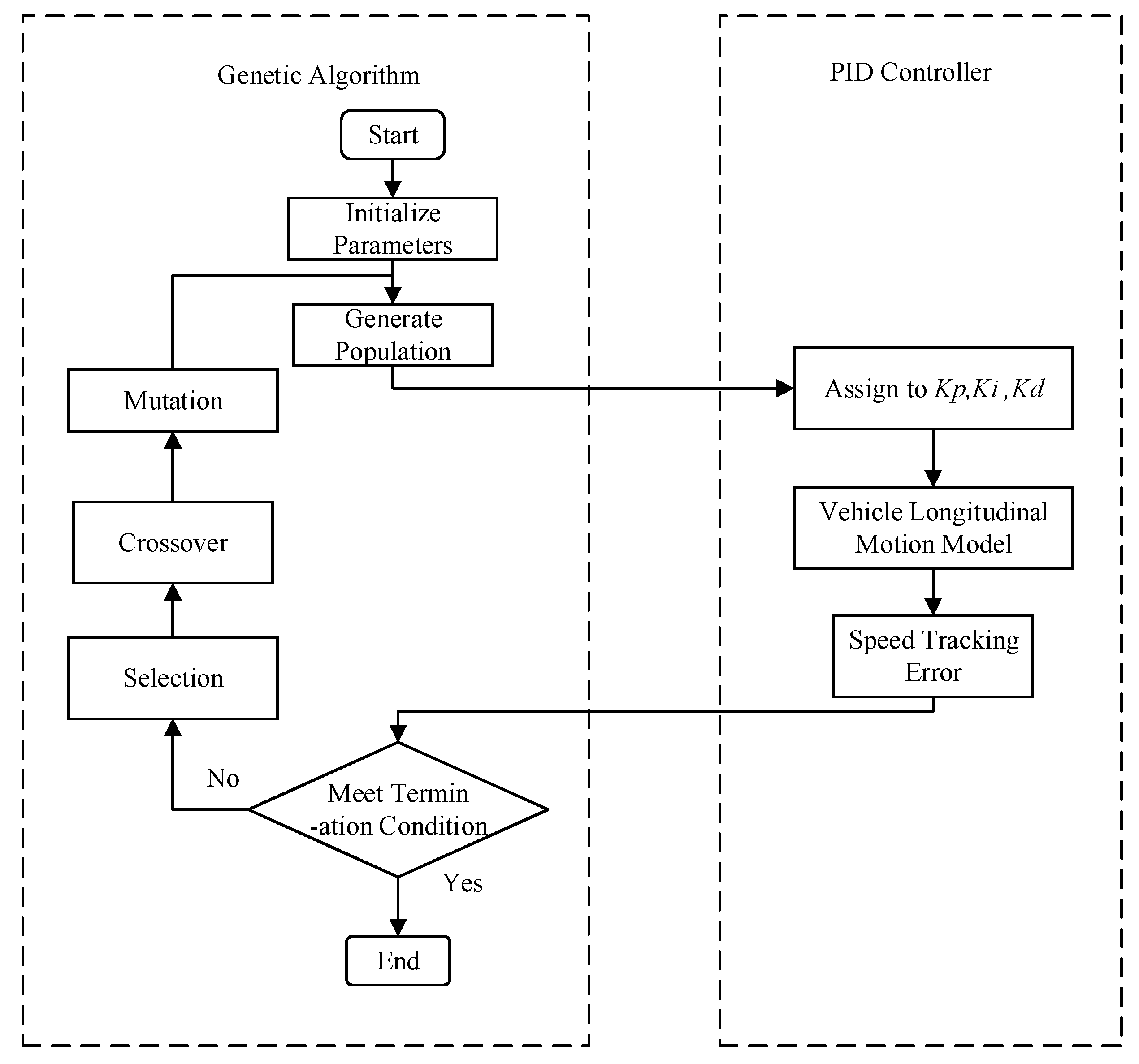
3.1. Basic Principles of Genetic Algorithm

The genetic algorithm is based on the principles of natural selection and genetic mechanisms from biological evolution theory. It solves optimization problems by simulating the processes of reproduction, mutation, and survival of the fittest. The basic steps are as follows:
  • Initialize Population: Randomly generate a set of possible solutions, with each individual representing one solution.
  • Fitness Evaluation: Use a fitness function to evaluate the quality of each individual.
  • Selection: Select the better individuals as parents based on their fitness, with higher chances for superior individuals to be chosen.
  • Crossover: Perform crossover operations between parent individuals to generate new individuals, combining genes from both parents.
  • Mutation: Randomly mutate some individuals to increase population diversity.
  • Iteration: Repeat the above steps to create a new population until the optimization conditions are met.
  • Output: The algorithm ultimately outputs the individual with the highest fitness as the optimal solution.
This process enables the genetic algorithm to progressively approach the global optimal solution.

3.2. Optimization Algorithm Design

The optimization goal of the genetic algorithm is to minimize the speed error during the speed tracking process of the autonomous vehicle. The speed error refers to the difference between the actual speed v a t and the desired speed v d t . The optimization objective function can be expressed as the sum of squared errors:
J = t = 1 N v a t v d t 2
where
  • J is the objective function, which represents the total error to be minimized;
  • v a t is the actual speed at time t ;
  • v d t is the desired speed at time t ;
  • N is the total time duration considered.
The flowchart of the optimization algorithm used in this study is shown in Figure 4.
  • Initialize the PID controller parameters and generate the initial population.
  • Input the PID controller parameters into the controller and simulate the longitudinal motion control process by controlling the vehicle’s speed.
  • Evaluate the performance of the current controller based on the error between the actual vehicle speed and the target speed.
  • Check if the error meets the termination condition. If it does, stop the optimization process and output the controller parameters. If not, proceed to the next step.
  • Select the better individuals based on the fitness function, with superior individuals having a higher chance of advancing to the next generation.
  • Perform crossover operations on the selected individuals to combine gene information from the parents, generating new individuals.
  • Apply gene mutation to the individuals in the population to increase diversity and help escape local optima.
  • Generate a new population consisting of multiple individuals, each representing a possible set of PID parameters, and reinput them into the PID controller.
The above steps 1–8 were programmed using MATLAB (2019b), and the corresponding code can be found in Appendix A.

4. Simulation Results and Discussion

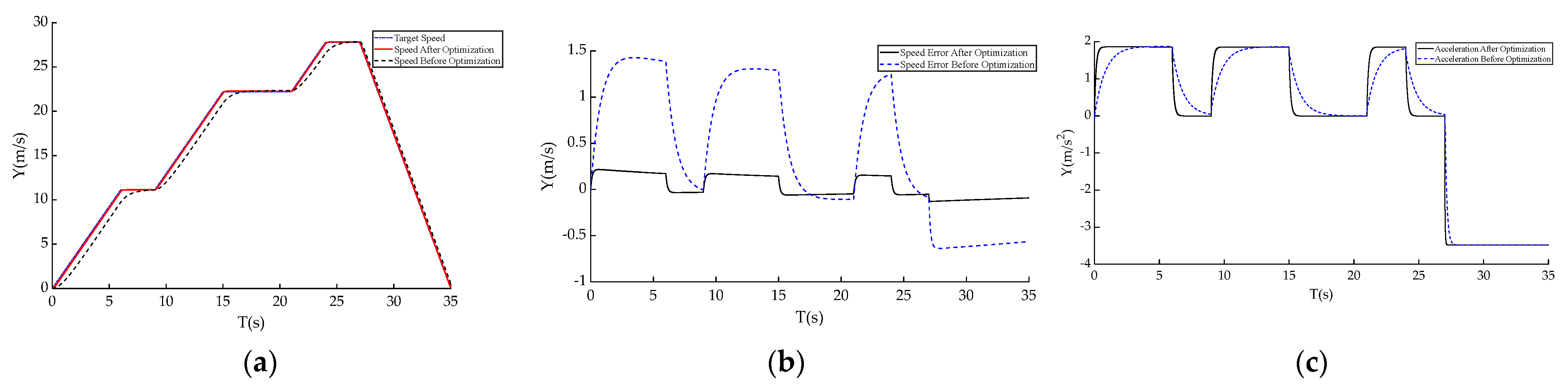
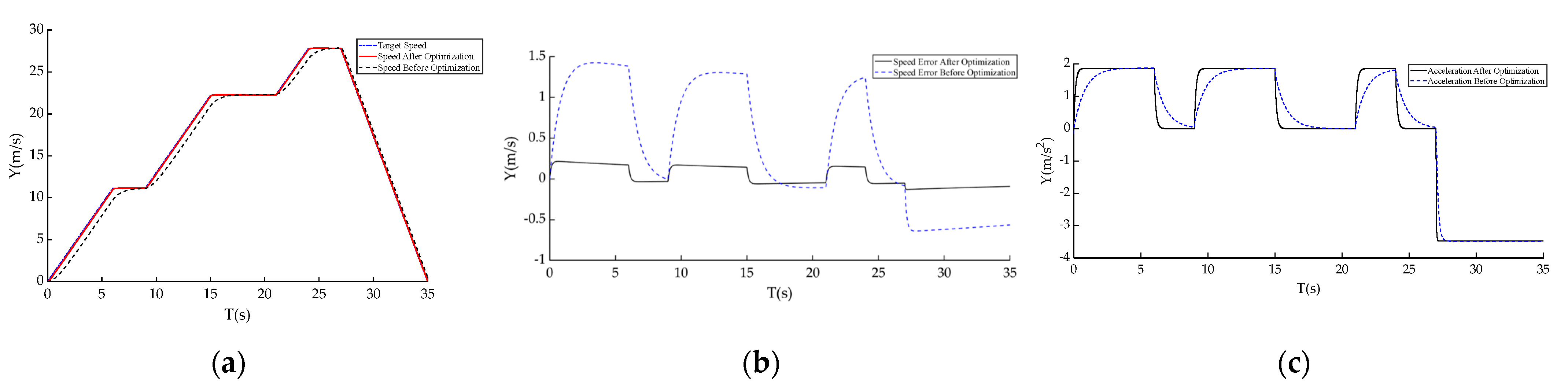
4.1. Experiment Design

In this study, a longitudinal PID control model for autonomous vehicles was constructed in the MATLAB/Simulink simulation (2019b) environment, with the model structure shown in Figure 3. The experiment focused on evaluating the longitudinal control performance of autonomous vehicles under varying road adhesion coefficients, selecting typical coefficient values of 0.5, 0.6, and 0.8 to simulate vehicle response behavior in low-, medium-, and high-adhesion environments. Through adjusting control parameters during the longitudinal acceleration and deceleration processes, the experiment analyzed the tracking performance of the controller’s speed under different road conditions.
Additionally, Table 1 presents the key parameters of the autonomous vehicle used in this experiment, including essential characteristics such as vehicle mass, providing an accurate physical foundation for the simulation model and ensuring the scientific rigor and reproducibility of the experimental results.
To implement the longitudinal control simulation experiment, the desired speed is set in segments to simulate the processes of acceleration, constant speed, and deceleration. The desired speed is set as follows:
  • 0–6 s: The vehicle accelerates from 0 km/h to 40 km/h, simulating the start-up acceleration process.
  • 6–9 s: The vehicle maintains a constant speed of 40 km/h for 3 s.
  • 9–15 s: The vehicle accelerates from 40 km/h to 80 km/h over 6 s, simulating the second phase of acceleration.
  • 15–21 s: The vehicle maintains a constant speed of 80 km/h for 6 s.
  • 21–24 s: The vehicle accelerates from 80 km/h to 100 km/h over 3 s, simulating the final phase of acceleration.
  • 24–27 s: The vehicle maintains a constant speed of 100 km/h for 3 s.
  • After 27 s: The vehicle begins to decelerate gradually from 100 km/h to 0 km/h, simulating the complete acceleration–deceleration process.

4.2. Error Analysis

In this study, 100 speed tracking simulation experiments were conducted under road surface adhesion coefficients of 0.5, 0.6, and 0.8. The set of parameters with the smallest speed tracking error for the autonomous vehicle was selected as the optimal parameters for the controller. K p = 136.36 , K i = 6.34 , and K i = 1.712 . The speed errors of the vehicle under different road surface adhesion coefficients with these parameters are shown in Table 2.
From Table 2, it can be seen that when the road surface adhesion coefficient is 0.5, the maximum speed tracking error of the autonomous vehicle is 0.22 m/s, the average error is 0.063 m/s, and the standard deviation is 0.124 m/s. When the road surface adhesion coefficient is 0.6, the maximum speed tracking error decreases to 0.18 m/s, the average error is 0.056 m/s, and the standard deviation is 0.099 m/s. When the road surface adhesion coefficient is 0.8, the maximum speed tracking error further decreases to 0.179 m/s, the average error remains at 0.056 m/s, and the standard deviation is 0.098 m/s.

4.3. Experimental Results Analysis

These results indicate that as the road adhesion coefficient increases, the speed tracking accuracy of the autonomous vehicle improves. This improvement is a direct result of the optimized PID controller parameters, which allow the vehicle to maintain a closer match to the desired speed, even under varying road conditions. The reduction in both maximum and average errors, as well as lower standard deviations, demonstrates that the optimization has significantly enhanced the overall performance of the controller, leading to more precise and stable speed regulation.
As shown in Figure 5a–c, under the condition where the road surface adhesion coefficient is 0.5, the desired speed range for the autonomous vehicle is 0–100 km/h, covering several common phases in daily driving, including low speed (0–30 km/h), medium speed (30–60 km/h), and high speed (above 60 km/h). Within this wide speed range, the autonomous vehicle applied the PID controller before and after parameter optimization for different scenarios: a 6 s acceleration, a 3 s acceleration, and an 8 s emergency deceleration.
The simulation results indicate that, during each acceleration and deceleration phase, the actual speed of the autonomous vehicle with optimized PID controller parameters closely follows the target speed, compared to before the PID parameter optimization. The error consistently remains within a small range. Particularly during multiple acceleration phases, the vehicle responds quickly and smoothly to changes in the target speed, demonstrating high speed tracking accuracy. Even in emergency deceleration scenarios, despite the rapid speed drop, the actual speed continues to closely track the target speed without significant overshoot or lag, highlighting the stability and robustness of the control system.
Moreover, as seen in Figure 5, the longitudinal dynamic response of the vehicle with optimized PID parameters during acceleration and deceleration is very smooth, with stable acceleration changes and no sudden fluctuations. This indicates that the PID controller parameter adjustment algorithm designed in this study not only improves the speed tracking accuracy of the PID controller but also significantly enhances the system’s dynamic response capability, enabling the autonomous vehicle to maintain stable and precise speed control across different speed ranges.
Therefore, based on this series of simulation results, it can be concluded that the proposed controller parameter optimization algorithm enables the autonomous vehicle to maintain excellent speed tracking performance under complex driving conditions while exhibiting high longitudinal control stability. This provides strong technical support for the practical application of autonomous vehicles in handling complex road conditions and dynamic changes, and lays a solid foundation for the further development of intelligent transportation systems.
As shown in Figure 6, under the condition where the road surface adhesion coefficient is 0.6, the desired speed range for the autonomous vehicle is 0–100 km/h, covering several common speed intervals in daily driving, including low speed (0–30 km/h), medium speed (30–60 km/h), and high speed (above 60 km/h). Within this relatively wide speed range, the autonomous vehicle, both before and after PID controller parameter optimization, underwent two 6 s acceleration phases, one 3 s acceleration phase, and one 8 s emergency deceleration phase.
The simulation results indicate that, during each acceleration and deceleration phase, the actual speed of the autonomous vehicle with optimized PID controller parameters is able to more closely follow the target speed compared to the vehicle without PID parameter optimization. The error consistently remains within a small range. Particularly during multiple acceleration phases, the optimized vehicle responds to changes in the target speed quickly and smoothly, demonstrating high speed tracking accuracy. Even in emergency deceleration phases, despite the rapid drop in speed, the actual speed still closely tracks the target speed without significant overshoot or lag, highlighting the stability and robustness of the control system.
Furthermore, as seen in Figure 6a, the longitudinal dynamic response of the vehicle controlled by the optimized PID controller is smoother during acceleration and deceleration. Figure 6b,c show that the vehicle’s acceleration changes are stable without sudden fluctuations when using the optimized PID controller. This demonstrates that the PID controller parameter optimization algorithm designed in this study not only effectively improves the speed tracking accuracy of the PID controller but also significantly enhances the system’s dynamic response capability, enabling the autonomous vehicle to maintain stable and precise speed control across different speed ranges.
Therefore, based on these simulation results, it can be concluded that the proposed controller parameter optimization algorithm enables the autonomous vehicle to achieve excellent speed tracking performance under complex driving conditions, while also demonstrating a high level of longitudinal control stability. This provides strong technical support for the practical application of autonomous vehicles in handling complex road conditions and dynamic changes, and lays a solid foundation for the future development of intelligent transportation systems.
As shown in Figure 7a–c, under the condition where the road surface adhesion coefficient is 0.8, the desired speed range for the autonomous vehicle is 0–100 km/h, covering multiple speed phases typical in daily driving, including low speed (0–30 km/h), medium speed (30–60 km/h), and high speed (above 60 km/h). Within this broad speed range, the vehicle used the PID controller both before and after parameter optimization, undergoing two 6 s acceleration phases, one 3 s acceleration phase, and one 8 s emergency deceleration phase.
The simulation results show that during each acceleration and deceleration phase, the actual speed of the autonomous vehicle with optimized PID controller parameters follows the target speed more effectively compared to the unoptimized controller. The error remains consistently small. Particularly during multiple acceleration phases, the optimized controller enables the vehicle to respond to changes in the target speed quickly and smoothly, demonstrating high speed tracking accuracy. Even during the emergency deceleration phase, despite the rapid drop in speed, the actual speed closely follows the target speed without significant overshoot or lag, highlighting the stability and robustness of the control system.
Additionally, from Figure 7, it can be seen that the PID controller with optimized parameters results in a very smooth longitudinal dynamic response throughout the acceleration and deceleration phases, with no sudden fluctuations in acceleration changes. This proves that the PID controller parameter optimization algorithm proposed in this study not only significantly improves the speed tracking accuracy of the PID controller but also greatly enhances the dynamic response capability of the system, allowing the autonomous vehicle to maintain stable and precise control across all speed ranges.
Therefore, based on this series of simulation results, it can be concluded that the proposed controller parameter optimization algorithm enables the autonomous vehicle to maintain excellent speed tracking performance under complex driving conditions while ensuring good longitudinal control stability. This provides strong technical support for the practical application of autonomous vehicles in dealing with complex road conditions and dynamic changes and lays a solid foundation for the future development of intelligent transportation systems.

5. Conclusions

This paper addresses the critical issue of speed control in autonomous vehicles and proposes a genetic algorithm-based PID controller parameter optimization method. The primary objective of this approach is to tackle the challenges associated with precise speed tracking in autonomous vehicles operating in complex and dynamic road environments. Speed tracking accuracy is essential to ensure that autonomous vehicles respond accurately and promptly to changing road conditions, thereby enhancing system safety, operational efficiency, and overall driving experience. This precision directly impacts passenger comfort and vehicle operational stability.
The proposed solution leverages the global search capabilities of genetic algorithms to achieve fine-tuning of PID controller parameters, significantly improving both speed control accuracy and the system’s dynamic response. Through this optimization, the autonomous vehicle can better adapt to various environmental conditions, such as road surface variations, further enhancing the vehicle’s stability and responsiveness, making it more reliable in real-world applications involving uncertainties.
Experimental results have clearly validated the effectiveness of this genetic algorithm-based optimization approach, particularly in terms of improved speed tracking accuracy, demonstrating that this method meets the complex control requirements of autonomous driving. However, to further clarify the applicability and potential prospects of this method, it is recommended that future studies verify its scalability and robustness in a broader range of real-world road conditions and multivariable control systems, thereby supporting its application in complex driving environments.

Author Contributions

J.C.: conceptualization, methodology, validation, writing—original draft preparation. G.T.: supervision, writing—reviewing and editing. All authors have read and agreed to the published version of the manuscript.

Funding

This research received no external funding.

Institutional Review Board Statement

Not applicable.

Informed Consent Statement

Not applicable.

Data Availability Statement

The data presented in this study are available on request from the corresponding author. The data are not publicly available due to privacy restrictions.

Conflicts of Interest

The authors declare no conflicts of interest.

Appendix A

Algorithm A1. PID Parameter Optimization Based on Genetic Algorithm
% Genetic Algorithm-based PID Parameter Optimization (Minimize Speed Error)
% Objective: Optimize PID parameters Kp, Ki, Kd

% Clear workspace
clear;
clc;

% Set Genetic Algorithm parameters
pop_size = 50;   % Population size
max_gen = 5;    % Maximum generations
pc = 0.7;     % Crossover probability
pm = 0.01;     % Mutation probability
bounds = [1 200;  % Range of Kp
     0 10;  % Range of Ki
     0 10];  % Range of Kd

% Initialize population
pop = init_population(pop_size, bounds);

% Set target speed (can be a constant value or based on model settings)
target_speed = 30; % Assume target speed is 30 m/s

% Main Genetic Algorithm loop
for gen = 1:max_gen
  % Calculate fitness
  fitness = zeros(pop_size, 1);
  for i = 1:pop_size
    params = pop(i, :);
    fitness(i) = fitness_function(params, target_speed); % Evaluate individual
  end
  
  % Select individuals
  selected_pop = selection(pop, fitness);
  
  % Crossover operation
  new_pop = crossover(selected_pop, pc, bounds);
  
  % Mutation operation
  new_pop = mutation(new_pop, pm, bounds);
  
  % Update population
  pop = new_pop;
  
  % Output best fitness of current generation
  [best_fitness, best_index] = min(fitness);
  best_params = pop(best_index, :);
  fprintf(‘Generation: %d, Best Fitness: %.4f, Best Parameters: [Kp = %.4f, Ki = %.4f, Kd = %.4f]\n’, …
    gen, best_fitness, best_params (1), best_params (2), best_params (3));
end

% Output final result
fprintf(‘Optimization complete, Best PID Parameters: Kp = %.4f, Ki = %.4f, Kd = %.4f\n’, …
  best_params (1), best_params (2), best_params (3));

%% Initialize Population Function
function pop = init_population(pop_size, bounds)
  num_params = size(bounds, 1);
  pop = zeros(pop_size, num_params);
  for i = 1:pop_size
    for j = 1:num_params
      pop(i, j) = bounds(j, 1) + rand × (bounds(j, 2) − bounds(j, 1));
    end
  end
end

%% Fitness Function (Objective Function − Minimize Speed Error)
function fitness = fitness_function(params, target_speed)
  Kp = params (1);
  Ki = params (2);
  Kd = params (3);

   % Set PID controller parameters
  assignin(‘base’, ‘Kp’, Kp);
  assignin(‘base’, ‘Ki’, Ki);
  assignin(‘base’, ‘Kd’, Kd);
  
  % Run Simulink model and get simulation results
  simOut = sim(‘vehicl_model_0910_2019b’, …
         ‘SimulationMode’, ‘normal’, …
         ‘SaveOutput’, ‘on’, …
         ‘SrcWorkspace’, ‘current’);
  
  % Extract vehicle speed and time data from simOut
  speed = simOut.vehicle_speed; % Extract vehicle speed
  time = simOut.tout;      % Extract time data

  % Calculate speed error
  speed_error = target_speed − speed;
  
  % Calculate Integral of Absolute Error (IAE) as fitness function
  IAE = sum(abs(speed_error) .× diff([0; time]));
  
  % Fitness function (smaller IAE is better)
  fitness = IAE;
end

%% Selection Function (Roulette Wheel Selection)
function selected_pop = selection(pop, fitness)
  pop_size = size(pop, 1);
  fitness_inv = 1./fitness; % Inverse fitness
  prob = fitness_inv/sum(fitness_inv); % Selection probability
  cum_prob = cumsum(prob); % Cumulative probability
  
  selected_pop = zeros(size(pop));
  for i = 1:pop_size
    r = rand;
    idx = find(cum_prob >= r, 1, ‘first’);
    selected_pop(i, :) = pop(idx, :);
  end
end

%% Crossover Function
function new_pop = crossover(pop, pc, bounds)
  pop_size = size(pop, 1);
  num_params = size(pop, 2);
  new_pop = pop;
  
  for i = 1:2:pop_size
    if rand < pc
      % Randomly select crossover point
      crossover_point = randi([1 num_params-1]);
      % Crossover operation
      new_pop(i, crossover_point + 1:end) = pop(i + 1, crossover_point + 1:end);
      new_pop(i + 1, crossover_point + 1:end) = pop(i, crossover_point + 1:end);
    end
  end
end

%% Mutation Function
function mutated_pop = mutation(pop, pm, bounds)
  pop_size = size(pop, 1);
  num_params = size(pop, 2);
  mutated_pop = pop;
  
  for i = 1:pop_size
    for j = 1:num_params
      if rand < pm
        mutated_pop(i, j) = bounds(j, 1) + rand × (bounds(j, 2) − bounds(j, 1));
      end
    end
  end
end

References

  1. Varma, B.; Swamy, N.; Mukherjee, S. Trajectory Tracking of Autonomous Vehicles using Different Control Techniques (PID vs. LQR vs. MPC). In Proceedings of the 2020 International Conference on Smart Technologies in Computing, Electrical and Electronics (ICSTCEE), Bengaluru, India, 9–10 October 2020. [Google Scholar]
  2. Liu, X.; Liang, J.; Fu, J. A dynamic trajectory planning method for lane-changing maneuver of connected and automated vehicles. Proc. Inst. Mech. Eng. Part D J. Automob. Eng. 2021, 235, 1808–1824. [Google Scholar] [CrossRef]
  3. Liu, Y.; Jiang, J. Optimum path-tracking control for inverse problem of vehicle handling dynamics. J. Mech. Sci. Technol. 2016, 30, 3433–3440. [Google Scholar] [CrossRef]
  4. Pang, H.; Liu, N.; Hu, C.; Xu, Z. A practical trajectory tracking control of autonomous vehicles using linear time-varying MPC method. Proc. Inst. Mech. Eng. Part D J. Automob. Eng. 2022, 236, 709–723. [Google Scholar] [CrossRef]
  5. Wang, Z.; Wei, C. Human-centred risk-potential-based trajectory planning of autonomous vehicles. Proc. Inst. Mech. Eng. Part D J. Automob. Eng. 2022, 237, 393–409. [Google Scholar] [CrossRef]
  6. Yin, J.-K.; Fu, W.-P. Framework of integrating trajectory replanning with tracking for self-driving cars. J. Mech. Sci. Technol. 2021, 35, 5655–5663. [Google Scholar] [CrossRef]
  7. Zhang, C.; Wang, C.; Wei, Y.; Wang, J. Neural network adaptive position tracking control of underactuated autonomous surface vehicle. J. Mech. Sci. Technol. 2020, 34, 855–865. [Google Scholar] [CrossRef]
  8. Calzolari, D.; Schürmann, B.; Althoff, M. Comparison of trajectory tracking controllers for autonomous vehicles. In Proceedings of the 2017 IEEE 20th International Conference on Intelligent Transportation Systems (ITSC), Yokohama, Japan, 16–19 October 2017. [Google Scholar]
  9. Zhu, Q.; Luo, Z.; Jiang, T.; Lu, Z.; Xia, M.; Hong, Y. Design and Motion Control of Six-Wheel Multi-Mode Mobile Robot. Trans. Chin. Soc. Agric. Mach. 2024, 1–8. [Google Scholar]
  10. Feng, G.; Zhao, D.; Li, S. Research on Air Spring Modeling and Active Suspension Control for Electric Vehicles Based on Fractional Order. Automot. Eng. 2024, 46, 1282–1293+1301. [Google Scholar]
  11. Li, J.; Pan, S.; Lou, J.; Li, Y.; Xu, Y. Application of Fuzzy PID Variable Structure Adaptive Algorithm in Vector Control of Steering Motor for Unmanned Vehicle. J. Electr. Mach. Control 2024, 28, 152–159. [Google Scholar]
  12. Wu, J.; Zhang, H. Fuzzy PID Control of Magnetorheological Brake with Dual-Coil Optimized by Genetic Algorithm. Automot. Eng. 2024, 46, 526–535. [Google Scholar]
  13. Lü, H.; Wang, X.; Xie, B.; Li, Q. Research on In-Place Steering Mechanism and Control Method of Distributed Electric Drive Vehicles. China J. Highw. Transp. 2024, 37, 231–244. [Google Scholar]
  14. Xiao, L.; Ma, L.; Huang, X. Intelligent fractional-order integral sliding mode control for PMSM based on an improved cascade observer. Front. Inform. Technol. Electron. Eng. 2022, 23, 328–338. [Google Scholar] [CrossRef]
  15. Lu, Y.; He, Y.; Tian, H.; Jiang, K.; Yang, D. Research on Longitudinal Acceleration Planning Method of Adaptive Cruise Control System for Mass Production. Automot. Eng. 2023, 45, 1803–1814. [Google Scholar]
  16. Li, Z.; Wang, X.; Jia, A. Fuzzy Adaptive PID Control of Cruise Ramjet-Extended Range Guided Projectile. Electro-Opt. Control 2023, 30, 22–28. [Google Scholar]
  17. Liu, S.; Yang, J.; Qin, Y.; Qi, H.; Shao, F. Robust Control Method for the Running Speed of Permanent Magnet Maglev Train Virtual Coupling. Rare Earths 2024, 45, 76–86. [Google Scholar]
  18. Yang, M.; Tian, J. Research on Adaptive Cruise Control of Pure Electric Vehicles. J. Chongqing Univ. Technol. (Nat. Sci.) 2023, 37, 19–26. [Google Scholar]
  19. Zhao, S.; Zhang, L.; Gan, Y.; Chen, W. Research on Hierarchical Control of Adaptive Cruise Control for Intelligent Electric Vehicles. J. Chongqing Jiaotong Univ. (Nat. Sci. Ed.) 2023, 42, 135–142. [Google Scholar]
  20. Ou, J.; Huang, D.; Lin, J.; Yang, E.; Han, X. Multi-Mode Adaptive Cruise Control Strategy with Emergency Braking Function. J. Chongqing Univ. Technol. (Nat. Sci.) 2023, 37, 57–68. [Google Scholar]
  21. Deng, L.; Lü, D. PID Parameter Tuning of Underwater Robot Motion Attitude Control Based on Genetic Algorithm. Manuf. Autom. 2023, 45, 177–179+206. [Google Scholar]
  22. Tao, J.; Lu, W.L.; Xiong, H. Improved Genetic Algorithm for PID Parameter Auto-Tuning. Ind. Instrum. Autom. Devices 2004, 2, 30–32. [Google Scholar]
  23. Liu, S.; Dan, Z.; Lian, B.; Xu, J.; Cao, H. PSO-PID Control Optimization Method for Interferometric Closed-Loop Fiber Optic Gyroscope. Infrared Laser Eng. 2024, 53, 250–261. [Google Scholar]
  24. Wu, Q.; Zhou, S.; Wang, X. Research on Improved Particle Swarm Optimization BP Neural Network PID Control Strategy for Ball Screw Feed System. J. Xi’an Jiaotong Univ. 2024, 58, 24–33. [Google Scholar]
  25. Editorial Department of China Journal of Highway and Transport. Summary of Academic Research on Automotive Engineering in China, 2023. China J. Highw. Transp. 2023, 36, 1–192. [Google Scholar]
  26. Wu, L. Design of Ship Turbine Speed Regulation System Combining Genetic Algorithm and PID Control. Ship Sci. Technol. 2021, 43, 100–102. [Google Scholar]
Figure 1. Force analysis diagram of longitudinal motion of an autonomous vehicle.
Applsci 14 10209 g001
Figure 2. PID control principle diagram.
Applsci 14 10209 g002
Figure 3. Longitudinal PID control model.
Applsci 14 10209 g003
Figure 4. Optimization algorithm flowchart.
Applsci 14 10209 g004
Figure 5. Simulation results for road adhesion coefficient 0.5. (a) Longitudinal speed. (b) Longitudinal speed error. (c) Longitudinal acceleration.
Applsci 14 10209 g005
Figure 6. Simulation results for road adhesion coefficient 0.6. (a) Longitudinal speed. (b) Longitudinal speed error. (c) Longitudinal acceleration.
Applsci 14 10209 g006
Figure 7. Simulation results for road adhesion coefficient 0.8. (a) Longitudinal speed. (b) Longitudinal speed error. (c) Longitudinal acceleration.
Applsci 14 10209 g007
Table 1. Vehicle parameters.
Mass1723 kg
Drag Coefficient0.3
Vehicle Frontal Area2.5 m2
Air Density1.225 kg/m3
Rolling Resistance Coefficient0.015
Gravitational Acceleration9.8 m/s2
Table 2. Speed errors of the autonomous vehicle after parameter optimization under different road surface adhesion coefficients.
Road Adhesion CoefficientMaximum
Value (m/s)
Average
Value (m/s)
Standard
Deviation (m/s)
0.50.2220.0630.124
0.60.1800.0560.099
0.80.1790.0560.098
Disclaimer/Publisher’s Note: The statements, opinions and data contained in all publications are solely those of the individual author(s) and contributor(s) and not of MDPI and/or the editor(s). MDPI and/or the editor(s) disclaim responsibility for any injury to people or property resulting from any ideas, methods, instructions or products referred to in the content.

