Abstract
There is growing international interest in assessing population exposure to radiofrequency electromagnetic fields, especially those generated by mobile-phone base stations. The work presented here is an experimental study in which we assess exposure to radiofrequency electromagnetic fields in a university environment, where there is a site with mobile-phone antennas and where a large number of people live on a daily basis. The data were collected with a personal exposure meter in two samplings, one walking at ground level and the other using an aerial vehicle at a height higher than the buildings. The geo-referenced electric-field data were subjected to a process in which a theoretical model was adjusted to the experimental variograms, and heat maps were obtained using kriging interpolation. The research carried out is of great relevance, since it provides detailed measurements of the electromagnetic radiation levels both at ground level and at significant heights, using innovative methodologies such as the use of drones. Furthermore, the results obtained allow for contextualizing the exposures in relation to international safety limits, highlighting the importance of rigorous monitoring in everyday environments.
1. Introduction
With the rapid growth of wireless communications, concerns about human exposure to electromagnetic fields (EMF) have gained significant attention. Mobile telephony, in particular, has become ubiquitous, leading to the proliferation of base stations and mobile devices, all of which emit radiofrequency (RF) radiation. The increasing density of these RF sources raises questions about the level of exposure in various environments, especially in urban areas where mobile base stations are positioned close to living and working spaces. As a result, it is crucial to monitor and evaluate the intensity of these electromagnetic fields to ensure that they remain within safe limits established by international standards, such as those provided by the International Commission on Non-Ionizing Radiation Protection (ICNIRP) [1].
One of the main challenges in evaluating exposure to electromagnetic fields lies in the complexity of the environments in which these measurements are conducted. Obstacles such as buildings, trees, and terrain can significantly influence the distribution and intensity of electromagnetic fields, leading to areas of both high and low exposure. Furthermore, exposure levels can vary not only at ground level but also at different heights, making it necessary to measure EMF levels in three-dimensional spaces to obtain a comprehensive understanding of exposure in any given area.
There are numerous instruments and measurement procedures for assessing human exposure to electromagnetic fields. Personal exposimeters (PEMs) have proven to be valuable tools in measuring individual exposure to RF radiation. These portable devices allow researchers to collect real-time data on electromagnetic field levels across multiple frequency bands. Initially, in personal dosimetry studies, PEMs were used attached to the body [2,3,4]. Recently, it has become possible to characterize exposure to electromagnetic fields in different micro-environments using vehicles, such as bicycles, cars, and drones [5,6,7,8,9]. However, PEM devices typically generate vast amounts of data, as they capture measurements in several frequency bands every few seconds. This wealth of information can complicate the analysis, as not all frequency bands provide meaningful data above the device’s detection threshold. To manage this, studies often focus on specific frequency bands that are relevant to the environment being studied, such as the frequencies used by nearby mobile base stations.
Although many studies have been carried out in different urban settings [6,10], few have been conducted in university areas [11,12,13]. The study we present here aims to assess the electric-field levels generated by a site with a mobile-phone base station located at the Polytechnic School of the University of Extremadura in Cáceres (Spain). The presence of mobile-phone antennas is expected to cause high levels of exposure to students, teachers and administrative and service staff, about 2500, who usually live there. We focused on bands commonly used by mobile networks for communication, and are essential in evaluating the exposure levels generated by mobile base stations. The findings will be compared to international safety guidelines to determine whether the measured levels fall within the recommended limits, ensuring the safety and well-being of individuals living or working near mobile base stations.
Given the environmental conditions of the study area, such as the presence of buildings and trees, it is expected that the electric-field levels will vary significantly between ground level and elevated heights. Previous research has indicated that exposure tends to increase with height [8,9] due to the height of the antenna above the ground and fewer obstructions between the measuring device and the source of radiation. In order to provide a more comprehensive view of the spatial distribution of EMF levels, measurements were conducted both at ground level and at 20 m height using a PEM attached to a drone. The collected data were analyzed using geostatistical methods, including kriging, which allows for the creation of continuous spatial distributions from discrete measurement points [14]. By comparing the electric-field levels measured at different heights and analyzing their spatial distribution, this study seeks to provide valuable insights into the factors that influence EMF exposure in urban environments.
2. Materials and Methods
The study was conducted at the Polytechnic School of the University of Extremadura, located on the university campus in the city of Cáceres, Spain (see Figure 1). It consists of seven buildings dedicated to teaching and research in the fields of telecommunications, computer science, building construction, and civil engineering. The study area has pedestrian pathways between each building that allow for user mobility and is surrounded by vegetation. It covers an area of approximately 32,000 m2 in a rectangular shape, including the perimeter encompassing all buildings, as well as the parking lots located to the north.
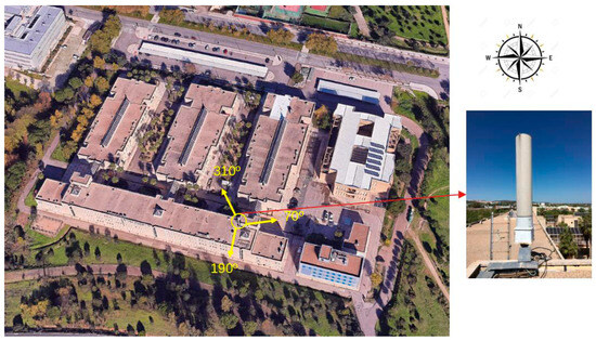
Figure 1.
Google Earth image of the Polytechnic School of the University of Extremadura in Cáceres, Spain. The location of the mobile base station antennas and the orientation of their sectors are indicated.
The central building, located on the southern side, has a mobile-phone base station on the roof, situated 17 m above the ground. The base station includes three sector antennas that cover a 120° angle each (see Figure 1) with a tilt angle of 4°. The antennas operate in different frequency bands associated with specific communication technologies. These bands are as follows: 842–852 MHz (4 G), 949.9–959.9 MHz (2 G/3 G), 1825–1845 MHz (2 G/4 G), and 2140–2155 MHz (3 G) [15]. The 700 MHz band (5 G) was not active at this site when the sampling was carried out in 2018, and will therefore not be considered in this study.
The geographic location of this base station makes it a strategic point for providing coverage to the entire Cáceres campus and its surroundings. However, it also exposes the study area to significant electromagnetic radiation emitted by the mobile base station antennas.
2.1. Personal Exposimeter
To measure the RF E-field, we used the personal exposimeter (PEM) EME SPY 200 (Microwave Vision Group, Courtaboeuf, France) [16]. It is lightweight and portable, with dimensions of 168.5 mm × 79 mm × 49.7 mm and a weight of 440 g. It consists of three orthogonal electric-field probes that continuously measure in 20 pre-defined frequency bands within the range of 87 MHz–5.85 GHz. The device can store up to 80,000 measurement points with a sampling interval between 4 and 255 s. It has a button to mark data points during measurements. It also integrates a GPS to geo-reference the locations where data are collected. Table 1 lists the technical specifications of this PEM, including frequency bands, sensitivity, and standard uncertainty due to axial isotropy in the vertical and horizontal planes for each band.

Table 1.
The technical specifications of the EME SPY 200 exposimeter, including frequency bands, sensitivity, and standard uncertainty due to axial isotropy in the vertical and horizontal planes. UL: uplink; DL: downlink.
2.2. Aerial Vehicle
Aerial measurements were performed by attaching the previously described PEM to a DJI S1000 drone using a plastic clamp (see Figure 2) (DJI, Shenzhen, China). The drone is a professional octocopter with a remote controller operating in the 2.4 GHz frequency band. It has a 15 min autonomy, a maximum takeoff weight of 11 kg, and includes the option of returning to its starting point in case the signal is lost. Additionally, we developed a system that allows for the remote pressing of the PEM button to mark points of interest for geo-referencing in the data file [13]. The drone’s structure and operation produce alterations in the electric-field measurements captured by the PEM, which were analyzed and quantified in a previous study [13]. The electric-field intensity readings were affected, and these distortions were corrected through correction factors. Additionally, wireless communication between the controller and the vehicle caused interference in the 2.4 GHz Wi-Fi band, but did not affect readings in the telephone bands.
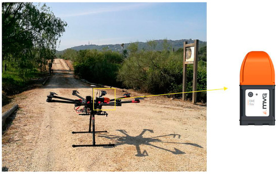
Figure 2.
EME SPY 200 exposimeter mounted on the DJI S1000 drone.
2.3. Data Collection
Two datasets were collected with the PEM, namely walking and using the aerial vehicle. In the first case, sampling was conducted with the operator moving at a constant speed, covering all pedestrian pathways at the Polytechnic School. The PEM was kept at a height of 1 m above ground level and away from the body at a distance of 0.5 m to minimize the effect of the human body on the measurements. The sampling interval was 4 s, and the total number of measurements was 331 (see Figure 3a). In the second case, the drone followed the same trajectory along the main pathways of the study area, as shown in Figure 3b. Sampling was carried out at a height of 20 m above the ground level referenced to the center of the Polytechnic School, exceeding the height of the surrounding buildings. It is important to note that there is a height difference of approximately 6 m between the parking lots to the north and the rest of the Polytechnic School, so measurements in the parking lot area were taken at a total height of 26 m above ground level. This is because the drone maintains a constant altitude from the initial takeoff point throughout the flight path. The sampling period was 4 s, and the total number of samples was 160.
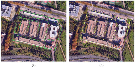
Figure 3.
Data collection points during walking sampling (a) and drone sampling (b).
2.4. Heat Maps
From the discrete electric-field data obtained in the aforementioned samplings, we generated continuous distributions to visualize the electric field in different frequency bands using heat maps. We employed the geostatistical method known as kriging, a stochastic technique that uses a linear combination of weights at known points to estimate values at unknown locations [14].
Geostatistics is a powerful tool for analyzing spatially distributed data and assumes that the variable under study is not entirely random but possesses a certain spatial structure. This spatial structure is typically analyzed by fitting a theoretical model to the experimental variogram. The variogram measures variability in terms of distance. A variogram, such as the one shown in Figure 4, is a graphical representation of variance as a function of the distance between points. In our case, if E(ri) and E(ri + h) represent the electric fields measured at two locations separated by a distance h, the variance γ(h) is defined by Equation (1) [14].
where N(h) is the number of data pairs [E(ri), E(ri + h)] separated by a distance h. When h = 0, the variance is zero because there are no differences between points compared with themselves. As h increases, the points are compared with others that are farther away, so the variance increases. At a certain distance, called the range (R), the variance γ(h) reaches a value γ(R) known as the sill, which is equivalent to the sample variance. For values of h greater than the range, the variance does not increase further, and the data can be considered independent. Theoretically, the variogram γ(h) should be zero when h = 0, but experimental variograms often present a positive value of γ(0), giving rise to the so-called nugget effect (see Figure 4). This effect can be caused by (i) microvariance or spatial variability at a scale smaller than that used for data collection, and (ii) experimental or sampling errors.
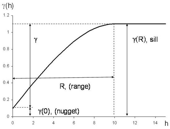
Figure 4.
Theoretical spherical variogram.
Fitting a theoretical model to the experimental variogram allows us to estimate the parameters R, γ(0), and γ(R), which can then be used to calculate electric-field values at unsampled points using kriging interpolation. This technique uses a weighted average of experimental data, where the weights depend not only on distance (as in distance-weighted averages) but also on the geometry of the sample locations, considering the spatial correlation structure deduced from the variogram analysis. The interpolated value, Einterp(r), at point r where no data were collected, is obtained using the linear estimator given by Equation (2).
where E(r1) and E(rN) are the known values at N locations and the weights λi are determined by minimizating the variance of the estimate [14]. The end result of kriging is a map including interpolated values of the variable.
3. Results and Discussion
The PEM generates a large amount of information, as it provides data in 20 frequency bands every four seconds. However, in most of them, the detected values do not exceed the equipment’s detection threshold (see Table 1). For this reason, we have focused solely on the telephony bands in which the mobile base station located at the Polytechnic School operates. These are the bands referred to in the personal exposimeter: LTE 800 DL, GSM + UMTS 900 DL, GSM 1800 DL, and UMTS 2100 DL. In both the walking measurements and those performed with the drone, we obtained all data above the detection threshold (0.005 V/m), which is logical given the proximity of the antenna to the measurement points.
Table 2 and Table 3 present statistical summaries of the electric-field levels recorded during the samplings conducted at ground level and with the drone, respectively, across the four mobile telephony bands. From these data, we note that the central parameters (mean and median) of the levels detected at 20 m height are between 2.9 and 4.4 times higher than those detected at ground level when comparing mean values, and between 3.1 and 4.8 times higher when using medians.
Table 2.
Statistical summary of the electric field measured at ground level in the four mobile-telephone bands. P25-P95 are the percentiles. SD: standard deviation. IQ: interquartile range. Sample size: 331.
Table 3.
Statistical summary of the electric field measured at 20 m height in the four mobile-telephone bands. P25-P95 are the percentiles. SD: standard deviation. IQ: interquartile range. Sample size: 160.
Regarding the maximum values, they were 0.968 V/m at ground level in the GSM + UMTS 900 DL band and 3.504 V/m at 20 m height in the UMTS 2100 DL band. To understand the significance of these values, we consider the reference levels from the ICNIRP 2020 standard, namely 41.25 and 58.34 V/m for the frequencies of 900 and 1800 MHz, respectively. Although our data cannot be directly compared to the ICNIRP 2020 standard (as it establishes reference levels for exposures averaged over 30 min and for whole-body exposure), we can conclude that they are clearly below the recommended limits.
Another noteworthy aspect of these tables is that in all cases (the four frequencies and the samples taken at ground level and at 20 m height), the standard deviation represents a high percentage (in some cases exceeding 100%) of the mean value. The same is true for the interquartile range and the median. This indicates that the data dispersion is high. Additionally, the mean values were higher than the medians in all cases, which is typical of non-Gaussian frequency distributions with positive skewness. Such distributions are very common in environmental data and are characterized by a large number of small values and few high values. As an example, Figure 5 shows the frequency distributions of the electric-field values in the GSM + UMTS 900 DL band in the samples at 20 m height. In the rest of the cases, the histograms showed a similar appearance.
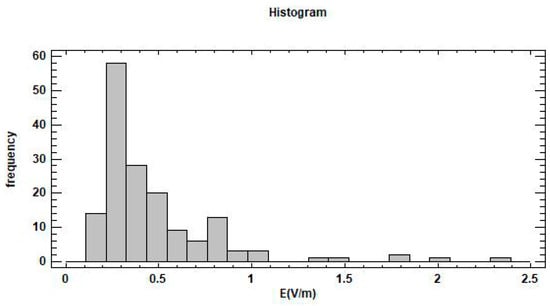
Figure 5.
Frequency distribution of the electric-field levels detected in the GSM + UMTS 900 DL band in the sampling carried out at a height of 20 m.
Based on the discrete data obtained experimentally, we constructed continuous distributions to visualize the electric field of the different frequency bands using heat maps. To achieve this, we used the kriging geostatistical method. This technique requires normal or quasi-normal frequency distributions, as abnormally high values increase the variance of the dataset. The variogram is very sensitive to these high values, and the lack of normality in the data can affect the accuracy of the kriging process [17].
However, data transformation techniques can be used to address the lack of normality. One solution to this problem is to transform the original data using functions like logarithms. Converting data to logarithms produces distributions that are approximately normal. In the field of radiocommunications, it is quite common to express units in decibels (dB). In these units, the electric field E(dB) is related to its value in the international system E(SI) by the equation E(dB) = 20 log[E(SI)]. In the following, we will use logarithmic units to address the issues that may arise when using non-normal distributions.
Using Equation (1), we obtained the experimental variograms corresponding to the four frequency bands and the two sampling taken. Figure 6 shows, as an example, the variogram corresponding to the GSM + UMTS 900 DL band at 20 m height, represented by points. There are 25 points in this variogram and each of them was calculated with between 60 and 320 pairs of experimental data. This allows us, according to Isaaks and Srivastava [18], to obtain reliable variograms.
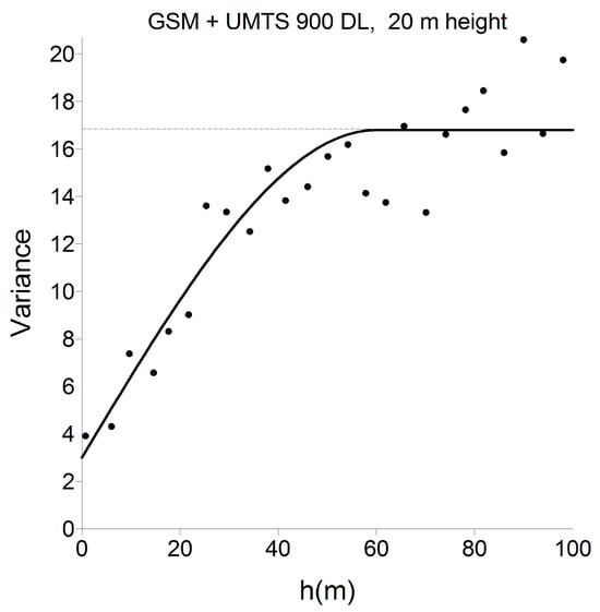
Figure 6.
Theoretical nugget + spherical variogram (solid line) fitted to the experimental variogram (dots) for the GSM + UMTS 900 DL band (20 m height). The dashed line represents the sample variance.
It can be observed in Figure 6 that the variance increases up to a certain distance, after which the increase slows down or even stabilizes. We also observe that the extrapolation of the data to the intercept with the y-axis (h = 0) does not pass through the origin. Therefore, the theoretical model we fitted to the experimental data is a spherical model (Equation (3) [14]) with a nugget effect γ(0), and is shown by a continuous line in Figure 6.
In this figure, it can be observed that γ(0) = 3 dB2, the range R = 60 m, and the total variance (sill) γ(R) = 17 dB2. Table 4 shows these parameters for the four frequency bands and the two samplings taken.
Table 4.
Nugget, γ(0), range, R, and sill, γ(R), obtained by fitting theoretical nugget + spherical variograms to the electric-field data of the four frequency bands and samplings at ground level and at 20 m height.
We highlight from these data that the total variance γ(R) at ground level is greater than that obtained with the drone at 20 m height. This may be due to the presence of buildings, trees, and uneven terrain. These elements cause areas with a direct line of sight to alternate with areas of shadow and this produces greater variability in the data. On the contrary, in the measurements taken with the drone, we are always in areas with a direct line of sight and this effect does not occur. As regards the parameter R, there are hardly any differences between both sets of data; in most cases, its value is between 60 and 70 m. On the other hand, the variance for h = 0, γ(0) takes values between 4 and 12 dB2 (standard deviation between 2 and 3.5 dB) in the sampling carried out at ground level, and slightly lower values, between 1 and 10 dB2 (SD between 1 and 3.2 dB) in the one carried out at 20 m height. These standard deviations are higher than the standard uncertainty for axial isotropy in the vertical and horizontal planes shown in Table 1, and therefore attributable to microvariance or experimental errors.
Based on the spatial dependence of the data given by the variograms, whose parameters are shown in Table 4, we created electric-field maps using kriging interpolation. The accuracy of the spatial kriging model in urban areas for electromagnetic levels was verified in a previous article [19].
The maps corresponding to the four frequency bands and the two samplings taken are shown in Figure 7 and Figure 8. In all cases, the same scale was used to facilitate data interpretation.
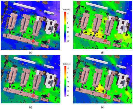
Figure 7.
Heat maps of electric-field intensities at ground level in the mobile-phone bands: (a) LTE 800 DL, (b) GSM + UMTS 900 DL, (c) GSM 1800 DL and (d) UMTS 2100 DL. The figures were obtained by merging the heat maps with aerial images of the area using Google Earth. The location of the site with sectorial mobile-phone antennas is shown in red along with the orientation of its sectors.
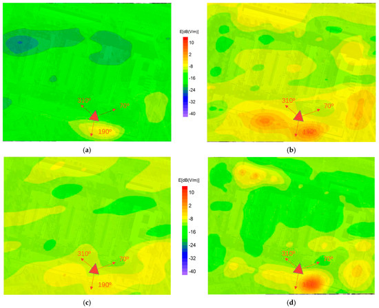
Figure 8.
Heat maps of electric-field intensities at 20 m height in the mobile-phone bands: (a) LTE 800 DL, (b) GSM + UMTS 900 DL, (c) GSM 1800 DL and (d) UMTS 2100 DL. The figures were obtained by merging the heat maps with aerial images of the area using Google Earth. The location of the site with sectorial mobile-phone antennas is shown in red along with the orientation of its sectors.
Figure 7 shows the maps, merged with Google Earth aerial images of the area, corresponding to the sampling carried out at ground level. The distribution of the electric-field levels is conditioned by the azimuth and inclination of the antennas, as well as by the existence of buildings and trees, which prevent a direct line of sight in some places. If we take as a reference the site with the mobile-phone antennas (in red in the figure), the highest electric-field values are located in the 70° and 310° directions, coinciding with two of the antenna sectors. On the other hand, in the 190° sector, no high values are detected. This is because the sampling points taken in the southern part of the sampling area are located in the “shadow” zone, since the building where the site is located prevents a direct line of sight with the antennas.
Figure 8 shows the electric-field maps at a height of 20 m. The images are semi-transparent so that the buildings can be seen, since their height is lower than that of the maps. In this sampling, carried out with the aerial vehicle, there are no obstacles that prevent the direct line of sight with the antenna, and the field levels are conditioned by the azimuth and inclination of the sectors. It can be observed in this figure that the highest values of the electric field in the four frequency bands are located at the bottom, where the site with mobile-telephone antennas is located.
Comparing the electric-field levels in both samples (Figure 7 and Figure 8), we observe that those detected with the PEM–drone system have higher values than those taken at ground level, which is in agreement with the data shown in Table 2. On average, the levels at 20 m were between 11 dB (LTE 800 DL, GSM + UMTS 900 DL, and UMTS 2100 DL bands) and 14 dB (GSM 1800 DL) higher than those taken at ground level.
4. Conclusions
From the results obtained, we can conclude that the electric-field levels recorded in the four mobile-phone bands evaluated are considerably lower than the reference limits established by the ICNIRP 2020 standard. Although the values detected at a height of 20 m are between 2.9 and 4.8 times higher than those recorded at ground level, they remain within safe margins for the general population. The high dispersion of the data, with positive asymmetry, suggests that the exposure levels are not uniform, but are influenced by the proximity to the antennas, the direct line of sight, and the configuration of the environment. The use of geo-statistical techniques such as kriging, together with the logarithmic transformation of the data, has made it possible to generate precise heat maps that illustrate the spatial variations of the electromagnetic field, which facilitates the identification of areas of greater exposure. Finally, the ability to perform sampling at different heights will allow for the experimental validation of propagation models, the safe monitoring of antenna emissions in their proximity, and, taking into account research on the attenuation of electromagnetic waves by buildings walls, the planning of indoor radio coverage and the evaluation of the exposure of the resident population to electromagnetic fields emitted by radio base stations.
Author Contributions
J.M.P.-S.: Conceptualization, Writing—Review and Editing, Supervision, Project Administration, Funding Acquisition. C.M.-C.: Methodology, Software, Investigation, Data Curation, Writing—Original Draft. F.J.G.-C.: Software, Formal Analysis, Investigation, Visualization. M.R.-P.: Resources, Writing—Review and Editing, Funding Acquisition. A.G.-G.: Validation, Investigation, Resources, Supervision. A.J.-B.: Resources, Writing—Review and Editing, Funding Acquisition. All authors have read and agreed to the published version of the manuscript.
Funding
This research was funded by the Extremadura Board and the European Regional Development Fund through the 5th Regional Technology Development and Innovation Research Plan (2014–2017), grant number GR15070.
Institutional Review Board Statement
Not applicable.
Informed Consent Statement
Not applicable.
Data Availability Statement
The original contributions presented in the study are included in the article, further inquiries can be directed to the corresponding author.
Acknowledgments
We thank the Extremadura Board and the European Regional Development Fund for the financial support provided through the 5th Regional Technology Development and Innovation Research Plan (2014–2017).
Conflicts of Interest
The authors declare no conflicts of interest.
References
- ICNIRP. Guidelines for Limiting Exposure to Electromagnetic Fields (100 kHz to 300 GHz). Health Phys. 2020, 118, 483–524. [Google Scholar] [CrossRef] [PubMed]
- Röösli, M.; Frei, P.; Mohler, E.; Braun-Fahrlander, C.; Burgi, A.; Frohlich, J.; Neubauer, G.; Theis, G.; Egger, M. Statistical analysis of personal radiofrequency electromagnetic field measurements with nondetects. Bioelectromagnetics 2008, 29, 471–478. [Google Scholar] [CrossRef] [PubMed]
- Frei, P.; Mohler, E.; Bürgi, A.; Fröhlich, J.; Neubauer, G.; Braun-Fahrländer, C.; Röösli, M. Classification of personal exposure to radio frequency electromagnetic fields (RF-EMF) for epidemiological research: Evaluation of different exposure assessment methods. Environ. Int. 2010, 36, 714–720. [Google Scholar] [CrossRef] [PubMed]
- Ibrani, M.; Hamiti, E.; Ahma, L.; Shala, B. Assessment of personal radio-frequency electromagnetic field exposure in specific indoor workplaces and possible worst-case scenarios. AEU Int. J. Electron. Commun. 2016, 70, 808–813. [Google Scholar] [CrossRef]
- Gonzalez-Rubio, J.; Arribas, E.; Ramirez-Vazquez, R.; Najera, A. Radiofrequency electromagnetic fields and some cancers of unknown etiology: An ecological study. Sci. Total Environ. 2017, 599–600, 834–843. [Google Scholar] [CrossRef] [PubMed]
- Sagar, S.; Adem, S.M.; Struchen, B.; Loughran, S.P.; Brunjes, M.E.; Arangua, L.; Dalvie, M.A.; Croft, R.J.; Jerrett, M.; Moskowitz, J.M.; et al. Comparison of radiofrequency electromagnetic field exposure levels in different everyday microenvironments in an international context. Environ. Int. 2018, 114, 297–306. [Google Scholar] [CrossRef] [PubMed]
- Paniagua-Sánchez, J.M.; García-Cobos, F.J.; Rufo-Pérez, M.; Jiménez-Barco, A. Large-area mobile measurement of outdoor exposure to radio frequencies. Sci. Total Environ. 2023, 877, 162852. [Google Scholar] [CrossRef] [PubMed]
- Joseph, W.; Aerts, S.; Vandenbossche, M.; Thielens, A.; Martens, L. Drone based measurement system for radiofrequency exposure assessment. Bioelectromagnetics 2016, 37, 195–199. [Google Scholar] [CrossRef] [PubMed]
- García-Cobos, F.J.; Paniagua-Sánchez, J.M.; Gordillo-Guerrero, A.; Marabel-Calderón, C.; Rufo-Pérez, M.; Jiménez-Barco, A. Personal exposimeter coupled to a drone as a system for measuring environmental electromagnetic fields. Environ. Res. 2023, 216, 114483. [Google Scholar] [CrossRef] [PubMed]
- Bhatt, C.R.; Thielens, A.; Billah, B.; Redmayne, M.; Abramson, M.J.; Sim, M.R.; Vermeulen, R.; Martens, L.; Joseph, W.; Benke, G. Assessment of personal exposure from radiofrequency-electromagnetic fields in Australia and Belgium using on-body calibrated exposimeters. Environ. Res. 2016, 151, 547–563. [Google Scholar] [CrossRef] [PubMed]
- Gil, I.; Fernandez-Garcia, R. Study of the exposure to time-varying electric field in the ESEIAAT UPC School. In Progress in Electromagnetic Research Symposium (PIERS); IEEE: Piscataway, NJ, USA, 2016; pp. 2184–2187. [Google Scholar] [CrossRef]
- Kljajic, D.; Djuric, N. Comparative analysis of EMF monitoring campaigns in the campus area of the University of Novi Sad. Environ. Sci. Pollut. Res. 2020, 27, 14735–14750. [Google Scholar] [CrossRef] [PubMed]
- Ramirez-Vazquez, R.; Escobar, I.; Martinez-Plaza, A.; Arribas, E. Comparison of personal exposure to Radiofrequency Electromagnetic Fields from Wi-Fi in a Spanish university over three years. Sci. Total Environ. 2023, 858, 160008. [Google Scholar] [CrossRef] [PubMed]
- Cressie, N.A.C. Statistics for Spatial Data; Revised Edition; John Wiley & Sons: New York, NY, USA, 1993. [Google Scholar]
- Gobierno de España, Ministerio de Industria, Energía y Turismo. Servicio de Información Sobre Instalaciones Radioeléctricas y Niveles de Exposición. Infoantenas. Available online: https://geoportal.minetur.gob.es/VCTEL/vcne.do (accessed on 26 September 2024).
- Microwave Vision Group. Courtaboeuf, France. Available online: https://www.temsystem.es/pdfs/EME_SPY_200.pdf (accessed on 26 September 2024).
- Sen, Z. Spatial Modeling Principles in Earth Sciences. Springer Science+Business Media B.V.: Berlin/Heidelberg, Germany, 2009. [Google Scholar]
- Isaaks, E.H.; Srivastava, R.M. Applied Geostatistics; Oxford University Press: Oxford, UK, 1989. [Google Scholar]
- Rufo, M.; Antolín, A.; Paniagua, J.M.; Jiménez, A. Optimization and comparison of three spatial interpolation methods for electromagnetic levels in the AM band within an urban area. Environ. Res. 2018, 162, 219–225. [Google Scholar] [CrossRef] [PubMed]
Disclaimer/Publisher’s Note: The statements, opinions and data contained in all publications are solely those of the individual author(s) and contributor(s) and not of MDPI and/or the editor(s). MDPI and/or the editor(s) disclaim responsibility for any injury to people or property resulting from any ideas, methods, instructions or products referred to in the content. |
© 2024 by the authors. Licensee MDPI, Basel, Switzerland. This article is an open access article distributed under the terms and conditions of the Creative Commons Attribution (CC BY) license (https://creativecommons.org/licenses/by/4.0/).