Article

Cervical Cancer Prediction Based on Imbalanced Data Using Machine Learning Algorithms with a Variety of Sampling Methods

by
Mădălina Maria Muraru
1,†,
Zsuzsa Simó
1,2,† and
László Barna Iantovics
2,*
1
Doctoral School of Letters, Humanities and Applied Sciences, George Emil Palade University of Medicine, Pharmacy, Science, and Technology of Targu Mures, 540142 Targu Mures, Romania
2
Department of Electrical Engineering and Information Technology, Faculty of Engineering and Information Technology, George Emil Palade University of Medicine, Pharmacy, Science, and Technology of Targu Mures, 540142 Targu Mures, Romania
*
Author to whom correspondence should be addressed.
These authors contributed equally to this work.
Appl. Sci. 2024, 14(22), 10085; https://doi.org/10.3390/app142210085
Submission received: 10 September 2024 / Revised: 23 October 2024 / Accepted: 29 October 2024 / Published: 5 November 2024

Abstract

:
Cervical cancer affects a large portion of the female population, making the prediction of this disease using Machine Learning (ML) of utmost importance. ML algorithms can be integrated into complex, intelligent, agent-based systems that can offer decision support to resident medical doctors or even experienced medical doctors. For instance, an experienced medical doctor may diagnose a case but need expert support that related to another medical specialty. Data imbalance is frequent in healthcare data and has a negative influence on predictions made using ML algorithms. Cancer data, in general, and cervical cancer data, in particular, are frequently imbalanced. For this study, we chose a messy, real-life cervical cancer dataset available in the Kaggle repository that includes large amounts of missing and noisy values. To identify the best imbalanced technique for this medical dataset, the performances of eleven important resampling methods are compared, combined with the following state-of-the-art ML models that are frequently applied in predictive healtchare research: K-Nearest Neighbors (KNN) (with k values of 2 and 3), binary Logistic Regression (bLR), and Random Forest (RF). The studied resampling methods include seven undersampling methods and four oversampling methods. For this dataset, the imbalance ratio was 12.73, with a 95% confidence interval ranging from 9.23% to 16.22%. The obtained results show that resampling methods help improve the classification ability of prediction models applied to cervical cancer data. The applied oversampling techniques for handling imbalanced data generally outperformed the undersampling methods. The average balanced accuracy for oversampling was 77.44%, compared to 62.28% for undersampling. When detecting the minority class, oversampling achieved an average score of 60.80%, while undersampling scored 41.36%. The logistic regression classifier had the greatest impact on balanced techniques, while random forest achieved promising performance, even before applying balancing techniques. Initially, KNN2 outperformed KNN3 across all metrics, including balanced accuracy, for which KNN2 achieved 53.57%, compared to 52.71% for KNN3. However, after applying oversampling techniques, KNN3 significantly improved its balanced accuracy to 73.78%, while that of KNN2 increased to 63.89%. Additionally, KNN3 outperformed KNN2 in minority class performance, scoring 55.72% compared to KNN2’s 33.93%.

1. Introduction

Cervical cancer is the fourth most commonly diagnosed cancer in women around the world [1]. According to [2], the most important risk factors and potential predictors of cervical cancer are smoking, infection with sexually transmitted diseases (HIV, syphilis, etc.), and the use of hormonal contraceptives. These risk factors underline the importance of using demographic and medical information as indicators for cervical cancer risk prediction. Analyzing these factors can help us to understand how lifestyle choices and medical conditions correlate with the development of cervical cancer.
Prediction, particularly classification, and, in general, decision making based on imbalanced datasets can lead to diverse difficulties in data mining [3,4]. The studies reported in [5,6,7] presented recent state-of-the-art methods for healthcare data-balancing issues, with promising results.
In this work, the main focus is on balancing issues in cervical cancer prediction based on messy, imbalanced data. One of the aims of this work was to study and compare a broad range of frequently applied data-balancing methods, combined with ML classification methods, and to evaluate the performance of these methods before and after balancing on the cervical cancer dataset. In the selection of the ML classification method, several key factors were taken into consideration. K-nearest neighbors makes local decisions, not using global patterns [8], and computationally efficient logistic regression is frequently used in medical research [9], while random forest can handle non-linear relationships well with ensemble learning [10]. These algorithms are widely used in healthcare research when dealing with imbalanced data. However, if scientists do not treat this problem appropriately, could lead to wrong research design.
This study investigated the following eight undersampling methods: Condensed Nearest Neighbor (CNN), Tomek Links (TLs), Edited Nearest Neighbor (ENN), Repeated Edited Nearest Neighbors (RENN), All K-Nearest Neighbors (All-KNN), NearMiss (NM), Neighborhood Cleaning Rule (NCR), and Instance Hardness Threshold (IHT). The following four oversampling methods were also studied: the Synthetic Minority Oversampling Technique (SMOTE); the Adaptive Synthetic Sampling Approach for Imbalanced Learning (ADASYN); methods based on the decision boundary, such as Support Vector Machine (SVM) and Borderline; and ML algorithms KNN, LR, and RF. By comparing these methods, we provide knowledge to improve classification accuracy while offering both experimental results and statistical characterization of the data.
This research subject is also motivated by the fact that in many studies include experimental evaluations of algorithms without characterization of the data to which they are applied. Such characterizations could provide a clear indication for other researchers regarding the applicability of algorithms to their specific data. Specifically, if the data have the respective characteristics, performance evaluation results similar to those reported in the research can be expected.
This research is presented under six main sections. Section 2 presents a state-of-the-art bibliographic study on balancing techniques with state-of-the-art classification algorithms in healthcare prediction. Section 3 outlines the steps of data preprocessing and the proposed classification methodology. Based on this, Section 4 presents the results achieved when applying the eleven studied sampling methods with the three studied ML methods, and Section 5 highlights the results in comparison with similar works. Finally, Section 6 summarizes the main ideas and proposes future work in the medical field.

2. Bibliographic Study

This section analyzes current state-of-the-art ML models in healthcare prediction (including cancer prediction) that are frequently mentioned among the best. Sampling methods, including oversampling and undersampling, can be applied in combination with these methods to improve accuracy and model performance. The main difference between over- and undersampling is that oversampling increases the size of the minority class with synthetic samples, while undersampling reduces the size of the majority class, which can lead to data loss. While prediction includes the act of predicting both numerical and categorical values, the goal of classification is specifically to predict a category, such as determining if a patient has a certain type of cancer or not.

2.1. Classification Algorithms

ML models are widely used in health care to predict diseases and analyze health records with the purpose of improving medical diagnoses. In this work, the following ML methods are studied: KNN, LR, and RF. These ML methods are widely used in medicine for disease prediction, disease classification, and risk assessment [11].

2.1.1. K-Nearest Neighbors Algorithm

KNN is independent of data distribution [8], since it makes predictions based on the local neighbors (where k is an integer, such as 2, 3, 4… and, in the case of KNN2 and KNN3, 2 and 3 are considered neighbors) of the data points without making assumptions about the sample size and the characteristics of the data. Algorithm A1 presents the process of KNN, including parameter initialization, computation of the distance, and majority vote classification. KNN might have problems with distance calculation when working with imbalanced data because it could capture more observations from the majority class [12].
Wang and Han [13] proposed a novel ensemble algorithm for an imbalanced Parkinson’s disease dataset, where the KNN is used as the base classifier to calculate the ensemble weights, which overcomes the challenges posed by differing severity levels given an imbalanced distribution of the data [14]. Fuzzy KNN combined with a Bonferroni mean classifier makes multiple comparisons between the input data, resulting in easier evaluation for high-dimensional datasets (microarray and COVID-19), with minimal numbers of features [15]. In Fuzzy KNN, the membership degree is calculated with fuzzy membership functions. The Bonferroni mean classifier is an aggregation operator.

2.1.2. Logistic Regression Algorithm

LR is used to determine the outcomes of a particular data point. In binary classification, LR predicts two possible outcomes, while in multiclass classification, the model can predict multiple classes. Binary (binomial) LR (bLR) is a specific form of LR [16], where the dependent variable has only two categories. The applicability of LR depends on the size of the dataset, meaning that when small, imbalanced datasets are used, LR can have biases towards the majority class, leading to incorrect prediction performance for the minority class.
Algorithm A2 presents the main method of LR. The advantages of the simple bLR algorithm is that there only simple hyperparameter tuning is required, such as tuning of the learning rate and the number of epochs. This algorithm might struggle with highly imbalanced data because it results in high accuracy and low recall or precision for the minority class. More advanced LR models include regularizations with penalty terms in order to keep the model’s weights small to prevent overfitting, but this leads to a decrease in accuracy [17].
To address this issue, Firth’s penalized LR introduces a penalty term in the traditional LR model to create parameter estimates and standard errors, resulting in improved model fitting in small, health survey-related datasets [9]. Ref. [18] presented a bLR classifier with 70% Principal Component Analysis (PCA) (dimensionality reduction of the dataset with 70% proportion of variance explained), which achieved the highest precision and sensitivity values when compared with Elastic Net, SVM with a linear kernel, SVM with a Radial Basis Function kernel, RF, and XGBoost. The researchers concluded that bLR performs well with quantitative imaging (CT and MRI scans to measure and analyze quantitative data) features as predictors. Besides predicting binary outcomes, LR can also be incorporated with Least Absolute Shrinkage and Selection Operator (Lasso) regularization. Lasso LR adds a rule that restricts the model from assigning importance to less relevant features [19].

2.1.3. Random Forest Algorithm

RF is an ensemble learning method used in classification that creates multiple decision trees during the process of training. Algorithm A3 represents the creation of bootstrap (random replacement subsets) samples for each decision tree for the forest. While creating a decision tree for each bootstrap, the algorithm selects a random subset of features and votes on the best split while it grows to the maximal depth. This random selection of features works better with imbalanced data because it reduces the overfitting of the majority class [20].
Yang and Fridgeirsson [10] used Lasso LR, RF, and XGBoost classifiers with random under- and oversampling methods and varied the target imbalance ratio. The study used four large health databases—three U.S. claims databases and one German EHR database, all mapped to the OMOP Common Data Model to investigate outcomes in patients with treated depression, where the initial sample was 100,000. After applying 58 prediction tasks on electronic health data, the results showed that only the models for random oversampling with RF showed more variation in the Receiver Operating Characteristic—Area Under the Curve (ROC-AUC) difference (which compares the performance of two classification models by quantifying how much better a model is able to separate positive and negative classes compared to another model).
Other works collected data through surveys, as demonstrated by Xin and Rashid [21], whose main goal was to predict depression among women, who may experience anxiety due to their life roles and physiological differences in Malaysia’s environment whereby women may face issues with money, family, health, and work. In this research, the authors used the SMOTE oversampling method with RF and concluded that the imbalance ratio affected the sensitivity of the RF model, which predicted disease accurately. RF can be applied in identifying longitudinal predictors of health and was able to discriminate poor from good self-perceived health outcomes in a 30-year cohort study [22].
According to the bibliographic study, in the medical field, LR is mostly used in cases of smaller datasets, while KNN and ensemble RF algorithms are applied in complex datasets with multiple attributes. The difference between them lies in their methodological approaches. The simple form of bLR’s parameters can be tuned easily, which works well with a lower number of features, while KNN and RF can capture interactions among features when patient data in medical research convey different types of information.

2.2. Sampling Methods

2.2.1. Undersampling Methods

To handle class imbalance, the following nearest neighbor-based methods were considered appropriate and were chosen for this study: CNN, TL, ENN, RENN, All-KNN, NM, NCR, and the iterative IHT method. For an accurate analysis, undersampling reduces the number of abundant observations to create two equally sized classes [13].
The CNN undersampling technique reduces the size of the majority class by keeping the most informative instances to maintain the decision boundary. The work reported in [23] used a one-pass variation of CNN called Instance-Based Learning 2 (IB2) and proposed a novel variation algorithm based on it. The researchers tested it on nine datasets, including variables with different types of data, some of which were related to the medical field (such as yeast, congenital heart disease, and water quality), achieving decreased computational cost for the multilabel classification process.
TL identifies pairs of observations from different classes that are the nearest neighbors to each other, but when combined with the SMOTE method, it can balance the training dataset and eliminate components that are on the wrong side of the decision. On a lung cancer dataset, this hybrid TL approach with balanced RF resulted in the highest mean AUC compared to other hybrid methods, including the baseline and SMOTE-Edited Nearest Neighbors (SMOTE-ENN) [24].
All-KNN removes observations from the majority class that have at least one nearest neighbor in the minority class to increase the separability of the classes. In a case study of the Parkinson’s Disease Tremor Severity Classification (a clinical dataset collected from a wearable sensor in laboratory and home environments), All-KNN with Artificial NN based on multi-layer perceptron (ANN-MLP) metrics such as accuracy, precision, and sensitivity improved, but the Index of Balanced Accuracy (IBA) and geometric mean stayed low [25].
RENN removes misclassified observations from the majority class until a desired class balance is achieved. The study reported in [11] used four imbalanced health datasets concerning diabetes, anemia, lung cancer, and obesity, featuring high-dimensional data with non-linear relationships. The researchers underlined that RENN with LR is more effective in handling the lack of symmetry in dataset distribution.
ENN is a cleaning technique but eliminates misclassified observations in one step without any iterative approach. A possible application of the ENN undersampling technique is in Medicare fraud detection. In [26], ENN was combined with SMOTE methods on the Medicare Part B dataset. The results showed that this hybrid approach effectively balanced synthetic observations while eliminating noisy data, and Decision Tree (DT) outperformed the following ML classifiers: Extreme Gradient Boosting (XGBoost), Adaptive Boosting (Adaboost), Light Gradient Boosting Machine (LGBM), LR, and RF.
The NCR technique removes misclassified majority observations and improves decision boundaries. In [27], a novel clustering approach was presented that improved the quality of classification. The authors used the K-Means algorithms to cluster the data; then, clusters of only the majority class at a specified distance from the center were removed. For the Yeast5 protein–protein interaction network dataset, the NCR method provided the best results in terms of the Matthews Correlation Coefficient (MCC) and Cohen’s Kappa statistic (Kappa) metrics.
The NM technique selectively removes majority-class instances based on the distances to minority-class instances (NM-1 removes the closest element, and NM-2 removes the farthest element from the minority class). Combining NM with PCA, Tumuluru and Daniel [28] presented a novel approach to address the class imbalance problem in healthcare data. Using a real-world dataset, the proposed model outperformed baseline classifiers in metrics like precision, recall, F1 Score, and AUC, highlighting possible applications in disease diagnosis, patient risk stratification, and treatment prediction. The work reported in [29] studied the problem of establishing the optimal number of factors in an Exploratory Factor Analysis (EFA) in general and PCA in particular, highlighting the complexity of the issue.
The IHT technique removes instances from the majority class and focuses on instances that are easier to classify while removing harder-to-identify observations. The work of Lopo and Hartomo [6] presented an evaluation of sampling techniques in healthcare insurance-related fraud detection, where the IHT method (with 90% class distribution) outperformed the XGBoost, SMOTE, and random oversampling methods overall, highlighting the ability to generalize well to new and unseen data in the minority and majority classes.

2.2.2. Oversampling Methods

For datasets with less information in particular classes to be balanced, artificial samples must be generated to increase the number of rare instances [30]. To create an equal class distribution by resizing the classes in this study, the following types of oversampling methods were used: methods based on the minority class, namely SMOTE and ADASYN, and methods based on the decision boundary, namely SVM and Borderline.
The SMOTE technique generates new instances of the minority class, resulting in improved performance in minority-class prediction. There are many varieties of SMOTE preprocessing techniques, namely traditional SMOTE, Borderline-SMOTE1, Borderline-SMOTE2, SMOTE-NC, and SVM-SMOTE, which were used in a hospital mortality prediction study of 126 patients with traumatic injuries. The data were extracted from the patients’ medical records. The researchers focused on the trauma patients’ status (alive/dead) as an outcome and six risk factors (age, sex, type of trauma, location of injuries, Glasgow coma scale, and white blood cells). The results showed that among all SMOTE-based ML methods, RF and ANN with SMOTE and XGBoost with SMOTE-NC achieved the highest values for all evaluation metrics [30]. Sinha [31] proposed a novel Data Augmented SMOTE Multi-Class Classifier (DASMcC) to predict Cardiovascular Diseases (CVDs). To ensure that the classifier’s performance was not biased, SMOTE was combined with a 10-fold cross-validation technique, while XGBoost performed the best overall.
SVM is an ML algorithm for binary classification, according to which the input vector performs a non-linear mapping process to create linearly separable data in a higher-dimensional feature space. Removing correlated features and simplifying the model-training process with PCA whitening results in data with unit variance along each dimension in the pretraining process of an imbalanced dataset [13]. Bektas [32] presented a novel ensemble model based on SVM’s hyperplane to calculate the optional boundaries between the signed distances integrated with bLR, resulting in higher accuracy compared to SVM kernel selection using datasets related to the ionosphere, High Time-Resolution Universe Survey (HTRU2) pulsar candidate, diabetes, and liver disorders.
Borderline oversampling is an advanced variation of SMOTE that generates samples near the decision boundaries of classes. Jo and Kim [5] proposed a novel method called minority oversampling near the borderline with a generative adversarial network (OBGAN) that uses Borderline with a generative adversarial network to focus on avoiding the mode-collapse problem on small datasets. Among 21 relatively small imbalanced datasets, examples of majority/minority outcomes include the following: liver cancer (have/not), with 10 features; breast cancer (benign/malignant), with 9 features; Pima Indian diabetes (diabetes/not), with 10 features; blood transfusion (not/donate), with 4 features (from the UCI ML Repository, Kaggle, and DataHub); and 6 benchmark methods (SMOTE, Borderline-SMOTE, ADASYN, k-means SMOTE (kmSMOTE), conditional GAN, and Generative Adversarial Minority Oversampling (GAMO). The experiments show OBGAN is competitive with the SMOTE-based methods and achieves stable performance for multiclass problems with various majority–minority ratios. The ADASYN technique adapts the generation process based on the density of the distribution of minority-class instances. Ahmed [33] proposed a DAD-net system to detect Alzheimer’s disease from images for which ADASYN was able to generate new samples to balance the number of instances in every category.
This section underlines the fact that databases of common health problems like cancer, Parkinson’s disease, and depression are widely used in the medical field for predictive purposes. However, some datasets are affected by common data issues such as missing values, outliers, and imbalanced data. To address this challenge, it is necessary to apply data manipulation techniques such as undersampling and oversampling. Some of available and innovative approaches incorporate algorithm modifications that have achieved promising results in healthcare prediction. For instance, SMOTE-ENN can eliminate noisy data in medical fraud detection, NCR with clustering can eliminate class objects in protein–protein datasets, and SMOTE data augmentation performs well for multiclass classification of CVDs.

3. Materials and Methods

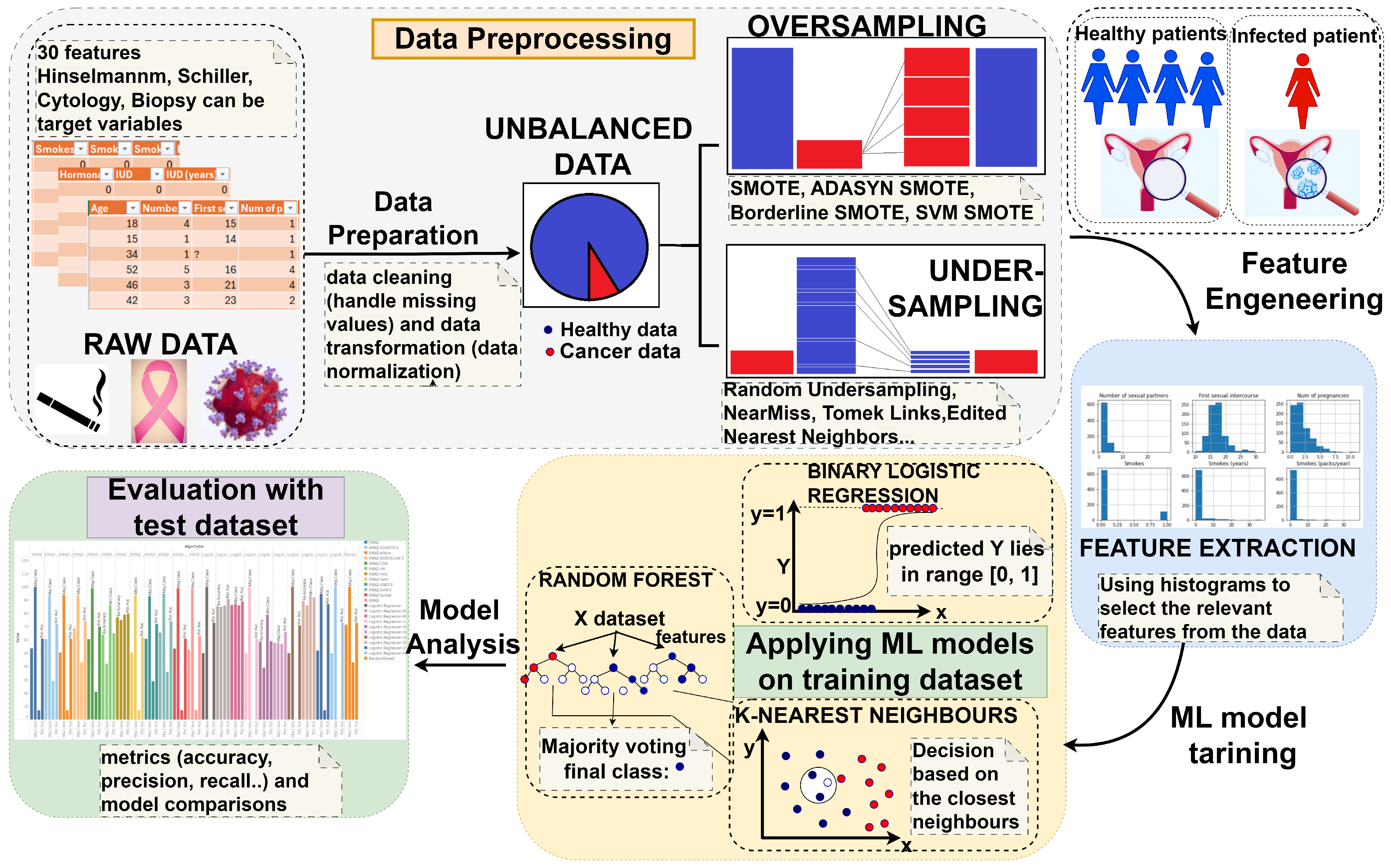
3.1. Conceptual Description

Figure 1 presents the research methodology and visually summarizes an ML workflow that includes data preprocessing, sampling, feature engineering, ML training, and model analysis. Our study outlines the performance of the KNN, LR, and RF methods combined with various undersampling and oversampling methods on a cervical cancer dataset with an Imbalance Ratio (IR) of 12.73 (the ratio of the number of instances in the majority class to the number of instances in the minority class). With only a 7% proportion with cancer, the 95% Confidence Interval (CI) for IR ranges between 9.23% and 16.22%. The dataset has over 2500 missing values.

3.2. Dataset Description

This study utilizes the cervical cancer risk factor dataset available on the UCI ML platform [34]. The data were collected from “Hospital Universitario de Caracas” in Caracas, Venezuela, comprising 858 records and 36 attributes (variables). The data reveal patients’ demographic information, habits, and medical history. The records contain the following four target variables: Hinselmann (screening test for abnormalities in the cervix) score, Schiller (identifying areas of concern with iodine test) score, and cytology (examination under a microscope for cell abnormality) and biopsy (for detection of the presence of cancer on removed tissue or cell samples) metrics. In this study, we selected biopsy as the only target variable. Because there were no data for cervical condylomatosis or AIDS, these two attributes were removed, leaving 30 variables as input.

3.3. Data Preprocessing

Clinical data are generally affected by factors such as missing values, inconsistent data, and exceptions, highlighting the need for preprocessing. Preprocessing is a very important step, as it includes both data preparation and data transformation. Tumuluru [28] recommended processing in different situation to change the distribution of the data and direct the algorithm.
Table 1 and Table A2 present the descriptive statistics of the dataset attributes, in integer and Boolean form, respectively. To ensure that every attribute contributed equally to the model training of the selected algorithms, the values were normalized in the [0, 1] interval. The calculation of the mean is presented in Equation (A1).
Missing information in the dataset can affect the statistical analysis. In the case of the used dataset, several patients refused to provide certain information; therefore, there are many missing values, especially in the case of very intimate questions like those concerning the use of hormonal contraceptives and intrauterine devices, as well as Sexually Transmitted Diseases (STDs).
After analyzing the data, it was evident that several missing values, especially intimate information, belong to the same patients, resulting in the elimination of 105 records, leaving 753 records from the original dataset. The remaining missing values were replaced with the median of the integer data and the most frequently occurring value for the Boolean data.
Figure 2 shows a graphical representation of the frequency distributions of several important attributes that were found to be the best predictors in the dataset. The figure also presents the result of the Lilliefors [35,36] numerical statistical test and estimations of the distribution in the case of the most important variables. Asymmetry to the right is visible, with a sudden decrease in the number of pregnancies per patient, i.e., women with zero, one, or two births. Similarly, for the number of years in which the patient used hormonal contraceptives, there is also an asymmetry to the right, caused by the generally young age of the women in the study. On the other hand, although the patients are relatively young, their age distribution is near symmetrical. The predominance of young age in the dataset may be explained by efforts to a culture of health awareness, where younger women are encouraged to participate in medical examinations and early cancer detection programs.
The Lilliefors test shows, experimentally, that the data follow a non-normal distribution, and because of this, the median was preferred over the mean [15]. The median is less sensitive to extreme values (outliers) than the mean, but there were no outliers in our dataset. In the case of binary variables, this approach is not suitable. A visual validation of the non-normal distribution is presented in Figure 3 using a Q-Q plot [37].
Another important aspect that can be identified immediately after data preprocessing is the number of instances in each class. The data distribution comprised 92% healthy patients and 7% of patients with a positive biopsy.
After data preprocessing, it is the imbalance ratio (IR) was calculated to measure the imbalance degree of the dataset, as expressed by I R = n negative n positive , where n negative is the number of negative samples and n positive is the number of positive samples, yielding a value of 12.73.
After this, the variance of the imbalance ratio can be approximated using the formula Var ( I R ) = I R 2 × 1 n positive + 1 n negative .
The Standard Error (SE) of the IR is expressed by S E ( I R ) = I R × 1 n positive + 1 n negative .
The 95% confidence interval (CI) for the IR is calculated as C I = I R ± Z × S E ( I R ) , where Z is the Z score corresponding to the desired confidence level (for 95%, Z = 1.96 ) and S E ( I R ) is the SE of the IR.
Finally, the lower and upper bounds of the CI are expressed by Lower Bound = I R Z × S E ( I R ) and Upper Bound = I R + Z × S E ( I R ) , yielding values of 9.23 and 16.22, respectively.

3.4. Model Training and Evaluation

These predictive models were implemented in the Python programming language using ML libraries. The Pandas library (version 1.5.3) was used for data manipulation and analysis, and Numpy (version 1.23.5) was employed for numerical calculations. For data visualization, Matplotlib (version 3.7.1) and Seaborn (version 0.12.2) were utilized. Interactive visualizations were created with Plotly (version 5.15.0), utilizing the Plotly.express module and the Plotly.io interface.
After processing the dataset, it was used to train NNs with four ML models (KNN with k values of 2 (KNN2) and 3 (KNN3), LR, and RF) utilizing Scikit-learn and Keras. The typical values for k in KNN are 2 or 3, but there is no unique, well-established strategy for determining the best k value [38]. We conducted experiments with a higher number of integers for K, but only values of 2 and 3 achieved notable results.
For the undersampling methods, the most relevant parameters were the sampling_ strategy (how many instances to sample for all methods), random_state (seed for random number generation like in a CNN), n_neighbours (number of neighbors to consider), and max_iter (limits the number of iterations), threshold_cleaning (decides which instance to keep). Oversampling methods include important parameters such as k_neighbors (number of nearest neighbors to use for synthetic sample generation for SVM and Borderline), m_neighbours (defining the number of neighbors to consider for SVM), and n_jobs (number of processors to use for parallel processing like in ADASYN). The values of the algorithms were selected based on the size of the data and class imbalance. Using guidelines established in [18] and empirical testing also improved model performance.
To measure model performance, we used a common ML approach where the data were split into a 75% training set and a 25% testing set. When evaluating models for the diagnosis of contagious diseases, such as sexually transmitted infections, which are a primary risk factor for cervical cancer, the selected metrics must align with the goals of diagnosis. In this case, identifying all the infected individuals (even at the risk of some false positives) is more critical than missing infected persons. In order to measure this imbalanced data learning, the following five evaluation metrics were selected as performance evaluation criteria: Accuracy (%) (A4), Precision (%) (A5), Recall (%) (A6), F1 Score (%) (A7), Balanced Accuracy (%) (Ba Accuracy) (A8) ROC_AUC score (%) [39], Class distribution (Majority (MajClass) or Minority Class (MinClass)), and Number of instances [40].
The confusion matrix presented in Table A1 represents the obtained classification results. Correctly classified instances are True Positive (TP) and True Negative (TN), and incorrectly classified instances are False Positive (FP) and False Negative (FN) [41].
The ROC curve and the corresponding AUC illustrate how well the model is capable of distinguishing between classes. The higher the AUC value, the more likely the model is to distinguish class 1 as 1 and class 0 as 0 (class 1 denotes cervical cancer; class 0 denotes cervical cancer not identified). To calculate it, a classifier and the probabilities obtained from predictions are needed. With multiple thresholds and based on each threshold, it can categorize the predicted probabilities as false or true and calculate the true-positive rate and false-positive rate.
An AUC closer to 1 indicates a better measure of separability, as well as which threshold is most suitable for a classifier, while the ROC curve is a probability curve. The X axis indicates the false-positive rate, and the Y axis represents the true-positive rate. Each point on the curve represents a probability threshold used to determine whether an example belongs to a certain category.
Metrics such as accuracy, F1 Score, and recall, both weighted and macro forms were also calculated to address the impact of imbalace. Macro metrics treat imbalanced classes as equals, highlighting the performance of the minority class. Weighted metrics represent the proportion of every class in the dataset, providing a measure of performance based on class frequency [42].
MacroPrecision (1), MacroRecall (2), and MacroF1score (3) represent the average precision, recall, and F1 Scores across all classes, respectively, as follows:
MacroPrecision = 1 N i = 1 N T P i T P i + F P i
MacroRecall = 1 N i = 1 N T P i T P i + F N i
MacroF 1 Score = 1 N i = 1 N 2 × T P i T P i + F P i × T P i T P i + F N i T P i T P i + F P i + T P i T P i + F N i
where N is the number of classes.
WeightedPrecision (4), MacroRecall (5), and WeightedF1score (6) represent the precision, recall and F1 Scores of each class weighted by the number of instances of that class, respectively, as follows:
WeightedPrecision = 1 i = 1 N | C i | i = 1 N T P i T P i + F P i × | C i |
WeightedRecall = 1 i = 1 N | C i | i = 1 N T P i T P i + F N i × | C i |
WeightedF 1 Score = 1 i = 1 N | C i | i = 1 N 2 × T P i T P i + F P i × T P i T P i + F N i T P i T P i + F P i + T P i T P i + F N i × | C i |
where | C i | is the number of instances in class i.

4. Results

The first experiment involved applying ML models using the original imbalanced dataset. For the other experiments, the balanced data were used with under- and oversampling techniques. The calculated weighted average (which gives more importance to values appearing more often in the data) used the numbers of data points in the majority and minority class as weights. On the other hand, the results of the macro average show the arithmetic mean of the metric values for each class, treating each class equally, regardless of the class size. Both averages are presented in Table 2, Table 3, Table 4, Table 5, Table 6, Table 7 and Table 8.
Table 2 reports the metric values obtained for all algorithms with the data in their state after initial preprocessing. We are interested in the highest values (numerical values represent percentages (%)). The obtained results show that the best performance was achieved by RF. The other classifiers, in general, are limited to predicting the minority class. The performance results of the ML models were obtained before applying sampling techniques.
Table 3 and Table 4 show the results obtained by the KNN algorithm with two neighbors after the application of under- and oversampling techniques. The highest sampling values for KNN were achieved by the Borderline SMOTE technique, but all methods generated much higher values than the models applied to the original dataset. ADASYN showed the least effectiveness overall, particularly in terms of accuracy and ROC_AUC score. These insights also suggest that SVM SMOTE is an effective oversampling technique for enhancing the performance of the KNN2 model. Among the undersampling techniques, NM1 and IHT predicted 78.57% and 85.71%, respectively. NCR stands out with a statistically significant ROC_AUC score of 0.80, which is notably higher than that of the rest. When excluding NCR, the remaining values do not show notable differences. The rest of the metric values were not higher than the original values.
Table A3 and Table 5 present the results achieved by KNN with three neighbors. For KNN3, every oversampling method worked well. In the case of undersampling, NM1 and IHT produced the best results, notably in the case of minority-class prediction. NM1 also excelled in class separation, with an ROC_AUC score of 0.79.
Table 6 and Table A4 present the results achieved by bLR. The good results for the AUC curve of all SMOTE methods must be noted. The undersampling techniques were not spectacular. CNN, TL, All-KNN, RENN, ENN, and NCR maintained high accuracy but at the cost of ignoring the minority class, resulting in poor balanced accuracy and macro metrics. NM1 and IHT handled the minority class better, but this came at the expense of overall accuracy.
Table 7 and Table 8 present the results obtained by RF. Although this algorithm proved effective and suitable for the initial data, after applying both types of sampling, it obtained further superior results. CNN and RENN offer a better balance, achieving high accuracy while maintaining reasonable performance for minority classes. It is also notable that the ADASYN and NM1 techniques achieved values of 85.71%, and 100%, respectively, in the detection of minority classes and ROC_AUC scores of more than 99% with all sampling methods.
A smaller area under the ROC curve is visible on the right side of Figure 4, and the left side shows the increase in the area under the ROC curve after applying the oversampling technique.

5. Discussions

5.1. Benefits of Prediction in Health Care

Using methods based on ML to solve diverse types of prediction problems can help health care to be more efficient and effective. In sophisticated data analytics, ML-based autonomous and intelligent systems are improved by intelligent communication technologies [43]. ML algorithms for prediction can help to develop preventive strategies in decision making, ensuring that the development of the algorithm is interpretable and transparent and takes into consideration ethical concerns [44].
Accuracy and real-time predictive analysis of disease prediction may lead to patients’ lives being saved, but incorrect predictions could endanger patients’ lives [45]. By integrating efficacious biomedical and health data, researchers can make accurate diagnoses based on ML methods to improve patient-centric treatments [46].

5.2. Advances in the Scientific Literature

Alsmariy [47] presented similar ML algorithms for cervical cancer prediction. The same dataset (used within our article) in this research was analyzed with PCA, balanced with SMOTE, and distributed with 10-fold cross-validation to prevent the overfitting problem. This approach raised the accuracy, sensitivity, and ROC_AUC score of the proposed model, a voting method that combines state-of-the-art classifiers: decision tree, logistic regression and random forest. Other cervical cancer work [1] used the dataset processed in this research, proposing a hybrid strategy based on the combination of an oversampling method (SMOTE) and two undersampling methods (CNN and ENN) to balance the dataset. Genetic algorithms were applied for feature selection, and RF classifier provided the highest performance in terms of G mean (geometric mean of the recall), sensitivity, and specificity.
In the case of a larger volume of data (more than 100,000 samples) or a large number of missing data (more than 10% of the data), diverse and sophisticated methods are available, including analyses to the replacement of missing values. For example, Entropy-Based (EB) algorithms, imputation of missing values, Independent Component Analysis (ICA), Linear Discriminant Analysis (LDA) [48], or the removal of outliers with covariance-based Mahalanobis distance, treating them as special values can be performed. A combination of these techniques is described in [49], the authors of which concluded that the ensemble model performed well under the proposed preprocessing and EB feature engineering method on a heart disease-related dataset including 14 features.

5.3. Results of This Research

We chose to use the traditional forms of KNN, LR, and RF because they are classic algorithms in ML. The bibliographic study showed that these algorithms have many improved versions, but they can also be complex or have potential disadvantages. Focusing on these algorithms, a clear comparison served as a basis for understanding their applicability.
The data analyzed in the experimental evaluation of this study were highly imbalanced, with 93% of the attributes belonging to the majority class and only 7% belonging to the minority class (positive biopsy cases). The CI with a 95% confidence level ranges between 9.23 and 16.22, while the the IB is 12.73. ML algorithms applied to the imbalanced data had difficulties detecting the minority class. One of the effects of imbalanced learning is that oversampling methods are more stable than other sampling methods (undersampling and hybrid sampling), while undersampling has is the least stable [24].
Evaluation of the imbalanced learning techniques applied to the dataset revealed that the use of oversampling techniques increased the performance of the models, proving to be inspired choices. KNN2 and KNN3 with undersampling initially predicted 7% of the minority class; after the application of sampling techniques, 86% of the majority class was predicted. LR improved from 0% to 93% with the SMOTE technique. Even for RF, which worked well even before applying the techniques, some metrics peaked. Decreasing the dimensionality of the dataset did not produce major changes, but some obtained metric values increased.
Based on the research that we performed, it can be concluded that the relationship between the minority and majority class is important in capturing each region in an imbalanced dataset while taking into consideration the sensitivity of ML in general and Neural Networks (NNs) in particular, which are more effective at learning the minority class with a focus near the borderline.

6. Conclusions

Based on the performed research, we conclude that datasets in a class with significantly fewer instances lead to overfit classifiers that favor the majority class. Based on this fact, the observations in the minority class are hardly recognizable or incorrectly identified. This issue is present in the medical field because, in many cases, the number of records corresponding to healthy patients (majority class) is much larger than the number of records for patients diagnosed with a specified disease (minority class). This leads to significant information related to minority classes corresponding to real-word medical problems being ignored, information that requires careful examination for prediction.
In our case, none of the studied oversampling methods (SMOTE, SVM SMOTE, Borderline SMOTE, or ADASYN), in combination with ML methods (KNN, LR, or RF) provided the best results in the case of any of the investigated evaluation metrics. KNN obtained higher metric values with the Borderline SMOTE method and RF than with the ADASYN method. It is also notable that in experiments, KNN3 performed better than KNN2. KNN3 achieved a balanced accuracy of 73.78%, while KNN2 scored 63.89%. KNN3 outperformed KNN2 in minority-class performance, scoring 55.72% compared to KNN2’s 33.93%. RF achieved good results with all oversampling methods, even before applying sampling techniques. This fact could lead to the use of compound classifiers in the future, although it is also important to pay attention to relevant attributes and eliminate irrelevant ones with the help of RF [22].
This paper presents a comprehensive research study of a large number of sampling methods used for data balancing with both over- and undersampling methods and discusses different modified versions. This study also serves as a practical guide for stakeholders because when using data with these characteristics, similar results can be expected when applying the investigated algorithms and balancing methods.
In future work, a set of hybrid classifiers (combining different classifiers and applying ensemble methods or feature-level hybridization with similar feature selection methods to PCA), in combination with under- and oversampling methods, could be be applied to the data used in this study.

Author Contributions

Conceptualization, Z.S., M.M.M. and L.B.I.; methodology, Z.S. and M.M.M.; software, M.M.M. and Z.S.; validation, M.M.M. and Z.S.; formal analysis, L.B.I. and M.M.M.; investigation, Z.S. and M.M.M.; resources, M.M.M.; data curation, M.M.M.; writing—original draft preparation, Z.S.; writing—review and editing, Z.S., M.M.M. and L.B.I.; visualization, M.M.M. and Z.S.; supervision, L.B.I.; project administration, L.B.I.; funding acquisition, Z.S. and L.B.I. All authors have read and agreed to the published version of the manuscript.

Funding

The article processing charge (APC) was funded by the Institution Organizing University Doctoral Studies (I.O.S.U.D.), the Doctoral School of Letters, Humanities, and Applied Sciences, George Emil Palade University of Medicine, Pharmacy, Science, and Technology of Târgu Mureş, 54014 Târgu Mureş, Romania.

Institutional Review Board Statement

Not applicable.

Informed Consent Statement

Not applicable.

Data Availability Statement

The datasets used in this article are publicly available for download at https://archive.ics.uci.edu/dataset/383/cervical+cancer+risk+factors (last accessed on 16 August 2024).

Acknowledgments

We would like to thank the Research Center on Artificial Intelligence, Data Science, and Smart Engineering (ARTEMIS) and COST Action CA22137—Randomised Optimisation Algorithms Research Network (ROAR-NET) for their support.

Conflicts of Interest

The authors declare no conflicts of interest.

Abbreviations

    The following abbreviations are used in this manuscript:
ADASYNAdaptive Synthetic Sampling Approach for Imbalanced Learning
All-KNNAll K-Nearest Neighbors
AUCArea Under the Curve
bLRBinary Logistic Regression
CIConfidence Interval
CNNCondensed Nearest Neighbor
EBEntropy-Based
ENNEdited Nearest Neighbors
IB2Instance-Based Learning 2
ICAIndependent Component Analysis
IHTInstance Hardness Threshold
IRImbalance Ratio
KNNK-Nearest Neighbors
LASSOLeast Absolute Shrinkage and Selection Operator
LDALinear Discriminant Analysis
LRLogistic Regression
MLMachine Learning
NCRNeighborhood Cleaning Rule
NNsNeural Networks
NMNearMiss
RFRandom Forest
RENNRepeated Edited Nearest Neighbors
ROCReceiver Operating Characteristic
SMOTESynthetic Minority Oversampling Technique
SVMSupport Vector Machine
TLTomek Links
ENNEdited Nearest Neighbors

Appendix A

Appendix A.1. Pseudocode of K-Nearest Neighbors Algorithm

Algorithm A1 K-Nearest Neighbors Algorithm [50]
1:
Input: D train : Training dataset; D test : Test dataset; k: Nr. of neighbors; d i s t _ m e t r i c
2:
Output: D predicted : Predicted labels for the test dataset
3:
Program Body
4:
for each x test in D test  do
5:
   let d i s t a n c e s be an empty list
6:
   for each x train in D train  do
7:
     let d i s t a n c e be d i s t _ m e t r i c ( x test , x train ) ;
8:
     let l a b e l be the label of x train ; append ( d i s t a n c e , l a b e l ) to d i s t a n c e s
9:
   end for
10:
   sort d i s t a n c e s by d i s t a n c e in ascending order; let k _ n e a r e s t be the first k elements from d i s t a n c e s ; let l a b e l _ c o u n t s be an empty dictionary
11:
   for each ( d i s t a n c e , l a b e l ) in k _ n e a r e s t  do
12:
     if label is not in l a b e l _ c o u n t s  then
13:
        let l a b e l _ c o u n t s [ l a b e l ] be 0
14:
     end if
15:
     increment l a b e l _ c o u n t s [ l a b e l ]
16:
   end for
17:
   let p r e d i c t e d _ l a b e l be the label with the highest count in l a b e l _ c o u n t s
18:
   assign p r e d i c t e d _ l a b e l to x test in D predicted
19:
end for
20:
Return   D predicted

Appendix A.2. Pseudocode of Logistic Regression Algorithm

Algorithm A2 Logistic Regression Algorithm [50]
1:
Input:   D train : Training dataset; D test : Test set; α : Learn rate; n _ e p o c h s : Training epochs
2:
Output: D predicted : Predicted probabilities for the test dataset
3:
Program Body
4:
Initialize θ (Parameter vector) to zero or random values
5:
for epoch = 1 to n _ e p o c h s  do
6:
   let g r a d i e n t s be a vector of zeros
7:
   for each ( x , y ) in D train  do
8:
     let z be the dot product of θ and x; let y ^ be the sigmoid function of z, y ^ = 1 1 + e z
9:
     let e r r o r be y ^ y ; update g r a d i e n t s by adding ( e r r o r · x )
10:
   end for
11:
   update θ by subtracting α · g r a d i e n t s
12:
end for
13:
Prediction for D test
14:
for each x test in D test  do
15:
   compute y ^ as the sigmoid of the dot product of θ and x test ; assign y ^ to D predicted
16:
end for
17:
Return   D predicted

Appendix A.3. Pseudocode of Random Forest Algorithm

Algorithm A3 Random Forest Algorithm [50]
1:
Input:   D train : Training dataset; D test : Test dataset; n _ t r e e s : Nr of trees in the forest; m a x _ d e p t h : Max depth of each tree; m i n _ s m p _ s p l i t and m i n _ s m p _ l e a f : Min and max nr of samples for leaf node
2:
Output: D predicted : Predicted labels for the test dataset
3:
Program Body
4:
Initialize an empty list f o r e s t : List of decision trees
5:
for tree = 1 to n _ t r e e s  do
6:
   let b o o t s t r a p _ s a m p l e be a random subset of D train (sampling with replacement)
7:
   let t r e e be a DT initialized with m a x _ d e p t h , m i n _ s m p _ s p l i t , and m i n _ s m p _ l e a f
8:
   train t r e e on b o o t s t r a p _ s a m p l e ; append t r e e to f o r e s t
9:
end for
10:
Prediction for D test
11:
for each x test in D test  do
12:
   let v o t e s be an empty dictionary
13:
   for each t r e e in f o r e s t  do
14:
     let p r e d i c t i o n be the result of t r e e on x test ; increment v o t e s [ p r e d i c t i o n ] by 1
15:
   end for
16:
   let p r e d i c t e d _ l a b e l be the label with the highest count in v o t e s ; assign p r e d i c t e d _ l a b e l to x test in D predicted
17:
end for
18:
Return   D predicted

Appendix B

The mean (A1) is calculated as follows:
mean = 1 N i = 1 N x i
where N is the number of observations and x i represents each observation. The standard deviation (A2) calculates the extent to which the numbers in the dataset are spread out from the mean.
stddev = 1 N i = 1 N ( x i mean ) 2
where mean is calculated. Based on Z score (A3), the normalization is expressed as follows:
x normalized = x mean stddev
where x is an individual data point and mean and stddev are the previously calculated values.

Model Evaluation Metrics

Table A1. Confusion matrix for binary classification.
ActualPrediction
PositiveNegative
PositiveTPFN
NegativeFPTN
Accuracy is the most commonly used metric in model evaluation and refers to the number of correctly labeled data points divided by the total number of examples. In other words, it is the rate of all predictions for both classes [41]. Accuracy for binary classification is expressed as follows:
Accuracy = T P + T N T P + T N + F P + F N
In the case of imbalanced data, accuracy is not a suitable metric when used in this form. If 1% of examples belong to the minority class, we can achieve an exaggerated accuracy of 99% by predicting the majority class [41].
The precision or positive predictive value for the binary case can be interpreted as being true in n% (it refers to the percentage of correct positive predictions) of cases, as follows:
Precision = T P T P + F P ,
and the reverse is called recall or the true-positive rate, corresponding to the number of correctly predicted positive samples or the number of correctly diagnosed patients with the disease [41].
Recall = T P T P + F N
The F1 Score is the weighted harmonic mean of precision and recall [41].
F 1 Score = 2 × R e c a l l × P r e c i s i o n R e c a l l + P r e c i s i o n
Ba accuracy is obtained from the rows of the confusion matrix and is the average recall for each distinct category in the dataset [41]. R e c a l l 0 = T P T P + F N , and R e c a l l 1 = T P T P + F N
Ba Accuracy = ( R e c a l l 0 + R e c a l l 1 ) 2 .

Appendix C

Appendix C.1. Dataset Description

Table A2. Count of binary data for attributes.
AttributeNegativePositiveMissingAttributeNegativePositiveMissing
Smokes72212313STDs: HIV73518105
Hormonal contraceptives269481108STDs: Hepatitis B7521105
IUD65883117STDs: HPV7512105
STDs67479105Dx:Cancer840180
STDs: condylomatosis70944105Dx:CIN84990
STDs: cervical condylomatosis7530105Dx:HPV840180
STDs: vaginal condylomatosis7494105Dx834240
STDs: vulvo-perineal condylomatosis71043105Hinselmann823350
STDs: syphilis73518105Schiller784740
STDs: pelvic inflammatory disease7521105Citology814440
STDs: genital herpes7521105Biopsy803550
STDs: molluscum contagiosum7521105STDs: AIDS7530105

Appendix C.2. Performance Results of KNN3 After Oversampling Techniques

Table A3. Performance results of KNN3 (after oversampling techniques).
Metric/SamplingSMOTESVM SMOTEBorderline SMOTEADASYN
Accuracy86.2489.9488.3587.30
Ba Accuracy72.8574.8574.0073.42
Precision (Mac;Wght)62.42;91.2567.26;92.1064.48;91.6963.54;91.46
Recall (Mac;Wght)72.85;86.2474.85;89.9474.00;88.3573.42;87.30
MajClass88.5792.5790.8689.71
MinClass57.1457.1457.1451.47
F1 Score (Mac;Wght)65.17;88.2470.08;90.8467.81;89.7266.44;88.98
ROC_AUC0.710.730.730.72

Appendix C.3. Performance Results of bLR After Undersampling Techniques

Table A4. Performance Results of bLR (after undersampling techniques).
Metric/SamplingCNNTLAll-KNNRENNENNNCRNM1IHT
Accuracy92.5992.5992.5992.5992.5992.5958.2041.79
Ba Accuracy50.0050.0050.0050.0050.0050.0057.7158.71
Precision (Mac;Wght)46.29;85.7346.29;85.7346.29;85.7346.29;85.7346.29;85.7346.29;85.7352.16;88.1852.54;89.37
Recall (Mac;Wght)50.00;92.5950.00;92.5950.00;92.5950.00;92.5950.00;92.5950.00;92.5957.71;58.2058.71;41.79
MajClass10010010010010010058.2938.86
MinClass00000057.1478.57
F1 Score (Mac;Wght)48.07;89.0348.07;89.0348.07;89.0348.07;89.0348.07;89.0348.07;89.0344.46;67.9935.97;67.99
ROC_AUC0.610.730.710.710.720.720.660.59
Note: Bolded values indicate significant performance for a metric.

References

  1. Newaz, A.; Muhtadi, S.; Haq, F.S. An intelligent decision support system for the accurate diagnosis of cervical cancer. Knowl. Based Syst. 2022, 245, 108634. [Google Scholar] [CrossRef]
  2. Bowden, S.J.; Doulgeraki, T.; Bouras, E.; Markozannes, G.; Athanasiou, A.; Grout-Smith, H.; Kechagias, K.S.; Ellis, L.B.; Zuber, V.; Chadeau-Hyam, M.; et al. Risk factors for human papillomavirus infection, cervical intraepithelial neoplasia and cervical cancer: An umbrella review and follow-up Mendelian randomisation studies. BMC Med. 2023, 21, 274. [Google Scholar] [CrossRef] [PubMed]
  3. Machado, D.; Santos Costa, V.; Brandão, P. Using Balancing Methods to Improve Glycaemia-Based Data Mining. In Proceedings of the 16th International Joint Conference on Biomedical Engineering Systems and Technologies (BIOSTEC 2023)—Volume 5: HEALTHINF; SciTePress: Setúbal, Portugal, 2023; pp. 188–198. [Google Scholar] [CrossRef]
  4. Alfakeeh, A.S.; Javed, M.A. Efficient Resource Allocation in Blockchain-Assisted Health Care Systems. Appl. Sci. 2023, 13, 9625. [Google Scholar] [CrossRef]
  5. Jo, W.; Kim, D. OBGAN: Minority oversampling near borderline with generative adversarial networks. Expert Syst. Appl. 2022, 197, 116694. [Google Scholar] [CrossRef]
  6. Lopo, J.A.; Hartomo, K.D. Evaluating Sampling Techniques for Healthcare Insurance Fraud Detection in Imbalanced Dataset. J. Ilm. Tek. Elektro Komput. Dan Inform. (JITEKI) 2023, 9, 223–238. [Google Scholar]
  7. Wang, W.; Chakraborty, G.; Chakraborty, B. Predicting the Risk of Chronic Kidney Disease (CKD) Using Machine Learning Algorithm. Appl. Sci. 2021, 11, 202. [Google Scholar] [CrossRef]
  8. Papakostas, M.; Das, K.; Abouelenien, M.; Mihalcea, R.; Burzo, M. Distracted and Drowsy Driving Modeling Using Deep Physiological Representations and Multitask Learning. Appl. Sci. 2021, 11, 88. [Google Scholar] [CrossRef]
  9. Suhas, S.; Manjunatha, N.; Kumar, C.N.; Benegal, V.; Rao, G.N.; Varghese, M.; Gururaj, G. Firth’s penalized logistic regression: A superior approach for analysis of data from India’s National Mental Health Survey, 2016. Indian J. Psychiatry 2023, 65, 1208–1213. [Google Scholar] [CrossRef]
  10. Yang, C.; Fridgeirsson, E.A.; Kors, J.A.; Reps, J.M.; Rijnbeek, P.R. Impact of random oversampling and random undersampling on the performance of prediction models developed using observational health data. J. Big Data 2024, 11, 7. [Google Scholar] [CrossRef]
  11. Awe, O.O.; Ojumu, J.B.; Ayanwoye, G.A.; Ojumoola, J.S.; Dias, R. Machine Learning Approaches for Handling Imbalances in Health Data Classification. In Sustainable Statistical and Data Science Methods and Practices; Awe, O.O., Vance, E.A., Eds.; Springer: Cham, Switzerland, 2023; pp. 19–33. [Google Scholar]
  12. Sajana, T.; Rao, K.V.S.N. Machine Learning Algorithms for Health Care Data Analytics Handling Imbalanced Datasets. In Handbook of Artificial Intelligence; Bentham Science Publishers: Potomac, MD, USA, 2023; p. 75. [Google Scholar]
  13. Wang, L.; Han, M.; Li, X.; Zhang, N.; Cheng, H. Review of Classification Methods on Unbalanced Data Sets. IEEE Access 2021, 9, 64606–64628. [Google Scholar] [CrossRef]
  14. Zhao, H.; Wang, R.; Lei, Y.; Liao, W.-H.; Cao, H.; Cao, J. Severity level diagnosis of Parkinson’s disease by ensemble K-nearest neighbor under imbalanced data. Expert Syst. Appl. 2022, 189, 116113. [Google Scholar] [CrossRef]
  15. Vommi, A.M.; Battula, T.K. A hybrid filter-wrapper feature selection using Fuzzy KNN based on Bonferroni mean for medical datasets classification: A COVID-19 case study. Expert Syst. Appl. 2023, 218, 119612. [Google Scholar] [CrossRef]
  16. Iantovics, L.B.; Enăchescu, C. Method for Data Quality Assessment of Synthetic Industrial Data. Sensors 2022, 22, 1608. [Google Scholar] [CrossRef] [PubMed]
  17. Lynam, A.L.; Dennis, J.M.; Owen, K.R.; Oram, R.A.; Jones, A.G.; Shields, B.M.; Ferrat, L.A. Logistic regression has similar performance to optimised machine learning algorithms in a clinical setting: Application to the discrimination between type 1 and type 2 diabetes in young adults. Diagn. Progn. Res. 2020, 4, 6. [Google Scholar] [CrossRef]
  18. Morgado, J.; Pereira, T.; Silva, F.; Freitas, C.; Negrão, E.; de Lima, B.F.; da Silva, M.C.; Madureira, A.J.; Ramos, I.; Hespanhol, V.; et al. Machine Learning and Feature Selection Methods for EGFR Mutation Status Prediction in Lung Cancer. Appl. Sci. 2021, 11, 3273. [Google Scholar] [CrossRef]
  19. Saharan, S.S.; Nagar, P.; Creasy, K.T.; Stock, E.O.; James, F.; Malloy, M.J.; Kane, J.P. Logistic Regression and Statistical Regularization Techniques for Risk Classification of Coronary Artery Disease Using Cytokines Transported by High Density Lipoproteins. In Proceedings of the 2023 International Conference on Computational Science and Computational Intelligence (CSCI), Las Vegas, NV, USA, 13–15 December 2023; pp. 652–660. [Google Scholar] [CrossRef]
  20. Ayoub, S.; Mohammed Ali, A.G.; Narhimene, B. Enhanced Intrusion Detection System for Remote Healthcare. In Advances in Computing Systems and Applications; Senouci, M.R., Boulahia, S.Y., Benatia, M.A., Eds.; Lecture Notes in Networks and Systems; Springer: Cham, Switzerland, 2022; Volume 513, pp. 1–11. [Google Scholar] [CrossRef]
  21. Xin, L.K.; Rashid, N.b.A. Prediction of Depression among Women Using Random Oversampling and Random Forest. In Proceedings of the 2021 International Conference of Women in Data Science at Taif University (WiDSTaif), Taif, Saudi Arabia, 30–31 March 2021; pp. 1–5. [Google Scholar] [CrossRef]
  22. Loef, B.; Wong, A.; Janssen, N.A.; Strak, M.; Hoekstra, J.; Picavet, H.S.; Boshuizen, H.H.; Verschuren, W.M.; Herber, G.C. Using random forest to identify longitudinal predictors of health in a 30-year cohort study. Sci. Rep. 2022, 12, 10372. [Google Scholar] [CrossRef]
  23. Filippakis, P.; Ougiaroglou, S.; Evangelidis, G. Prototype Selection for Multilabel Instance-Based Learning. Information 2023, 14, 572. [Google Scholar] [CrossRef]
  24. Khushi, M.; Shaukat, K.; Alam, T.M.; Hameed, I.A.; Uddin, S.; Luo, S.; Yang, X.; Reyes, M.C. A Comparative Performance Analysis of Data Resampling Methods on Imbalance Medical Data. IEEE Access 2021, 9, 109960–109975. [Google Scholar] [CrossRef]
  25. AlMahadin, G.; Lotfi, A.; Carthy, M.M.; Breedon, P. Enhanced Parkinson’s Disease Tremor Severity Classification by Combining Signal Processing with Resampling Techniques. SN Comput. Sci. 2022, 3, 63. [Google Scholar] [CrossRef]
  26. Bounab, R.; Zarour, K.; Guelib, B.; Khlifa, N. Enhancing Medicare Fraud Detection Through Machine Learning: Addressing Class Imbalance With SMOTE-ENN. IEEE Access 2024, 12, 54382–54396. [Google Scholar] [CrossRef]
  27. Bach, M.; Trofimiak, P.; Kostrzewa, D.; Werner, A. CLEANSE—Cluster-based Undersampling Method. Procedia Comput. Sci. 2023, 225, 4541–4550. [Google Scholar] [CrossRef]
  28. Tumuluru, P.; Daniel, R.; Mahesh, G.; Lakshmi, K.D.; Mahidhar, P.; Kumar, M.V. Class Imbalance of Bio-Medical Data by Using PCA-Near Miss for Classification. In Proceedings of the 2023 5th International Conference on Inventive Research in Computing Applications (ICIRCA), Coimbatore, India, 3–5 August 2023; pp. 1832–1839. [Google Scholar] [CrossRef]
  29. Iantovics, L.B.; Rotar, C.; Morar, F. Survey on establishing the optimal number of factors in exploratory factor analysis applied to data mining. Wiley Interdiscip. Rev. Data Min. Knowl. Discov. 2019, 9, e1294. [Google Scholar] [CrossRef]
  30. Hassanzadeh, R.; Farhadian, M.; Rafieemehr, H. Hospital mortality prediction in traumatic injuries patients: Comparing different SMOTE-based machine learning algorithms. BMC Med. Res. Methodol. 2023, 23, 101. [Google Scholar] [CrossRef] [PubMed]
  31. Sinha, N.; Kumar, M.A.G.; Joshi, A.M.; Cenkeramaddi, L.R. DASMcC: Data Augmented SMOTE Multi-Class Classifier for Prediction of Cardiovascular Diseases Using Time Series Features. IEEE Access 2023, 11, 117643–117655. [Google Scholar] [CrossRef]
  32. Bektaş, J. EKSL: An effective novel dynamic ensemble model for unbalanced datasets based on LR and SVM hyperplane-distances. Inf. Sci. 2022, 597, 182–192. [Google Scholar] [CrossRef]
  33. Ahmed, G.; Er, M.J.; Fareed, M.M.; Zikria, S.; Mahmood, S.; He, J.; Asad, M.; Jilani, S.F.; Aslam, M. DAD-Net: Classification of Alzheimer’s Disease Using ADASYN Oversampling Technique and Optimized Neural Network. Molecules 2022, 27, 7085. [Google Scholar] [CrossRef]
  34. Cervical Cancer (Risk Factors) Data Set. Available online: https://archive.ics.uci.edu/dataset/383/cervical+cancer+risk+factors (accessed on 1 October 2024).
  35. Pinheiro, V.C.; do Carmo, J.C.; de O. Nascimento, F.A.; Miosso, C.J. System for the analysis of human balance based on accelerometers and support vector machines. Comput. Methods Programs Biomed. Update 2023, 4, 100123. [Google Scholar] [CrossRef]
  36. Iantovics, L.B.; Dehmer, M.; Emmert-Streib, F. MetrIntSimil—An Accurate and Robust Metric for Comparison of Similarity in Intelligence of Any Number of Cooperative Multiagent Systems. Symmetry 2018, 10, 48. [Google Scholar] [CrossRef]
  37. Darville, J.; Yavuz, A.; Runsewe, T.; Celik, N. Effective sampling for drift mitigation in machine learning using scenario selection: A microgrid case study. Appl. Energy 2023, 341, 121048. [Google Scholar] [CrossRef]
  38. Ibrahim, K.S.M.H.; Huang, Y.F.; Ahmed, A.N.; Koo, C.H.; El-Shafie, A. A review of the hybrid artificial intelligence and optimization modelling of hydrological streamflow forecasting. Alex. Eng. J. 2022, 61, 279–303. [Google Scholar] [CrossRef]
  39. Naidu, G.; Zuva, T.; Sibanda, E.M. A Review of Evaluation Metrics in Machine Learning Algorithms. In Artificial Intelligence Application in Networks and Systems (CSOC 2023); Silhavy, R., Silhavy, P., Eds.; Lecture Notes in Networks and Systems; Springer: Cham, Switzerland, 2023; Volume 724. [Google Scholar] [CrossRef]
  40. Chen, R.J.; Wang, J.J.; Williamson, D.F.; Chen, T.Y.; Lipkova, J.; Lu, M.Y.; Sahai, S.; Mahmood, F. Algorithmic fairness in artificial intelligence for medicine and healthcare. Nat. Biomed. Eng. 2023, 7, 719–742. [Google Scholar] [CrossRef] [PubMed]
  41. Ng, A.P.; Koumchatzky, N. Machine Learning Engineering with Python, 2nd ed.; Packt Publishing: Birmingham, UK, 2023; 462p, ISBN 9781837631964. [Google Scholar]
  42. Edward, J.; Rosli, M.M.; Seman, A. A New Multi-Class Rebalancing Framework for Imbalance Medical Data. IEEE Access 2023, 11, 92857–92874. [Google Scholar] [CrossRef]
  43. Manchadi, O.; Ben-Bouazza, F.-E.; Jioudi, B. Predictive Maintenance in Healthcare System: A Survey. IEEE Access 2023, 11, 61313–61330. [Google Scholar] [CrossRef]
  44. Rubinger, L.; Gazendam, A.; Ekhtiari, S.; Bhandari, M. Machine learning and artificial intelligence in research and healthcare. Injury 2023, 54 (Suppl. 3), S69–S73. [Google Scholar] [CrossRef]
  45. Badawy, M.; Ramadan, N.; Hefny, H.A. Healthcare predictive analytics using machine learning and deep learning techniques: A survey. J. Electr. Syst. Inf. Technol. 2023, 10, 40. [Google Scholar] [CrossRef]
  46. Subrahmanya, S.V.; Shetty, D.K.; Patil, V.; Hameed, B.Z.; Paul, R.; Smriti, K.; Naik, N.; Somani, B.K. The role of data science in healthcare advancements: Applications, benefits, and future prospects. Ir. J. Med. Sci. 2022, 191, 1473–1483. [Google Scholar] [CrossRef]
  47. Alsmariy, R.; Healy, G.; Abdelhafez, H. Predicting Cervical Cancer using Machine Learning Methods. Int. J. Adv. Comput. Sci. Appl. (IJACSA) 2020, 11, 7. [Google Scholar] [CrossRef]
  48. Toğaçar, M.; Ergen, B.; Cömert, Z.; Özyurt, F. A Deep Feature Learning Model for Pneumonia Detection Applying a Combination of mRMR Feature Selection and Machine Learning Models. Irbm 2020, 41, 212–222. [Google Scholar] [CrossRef]
  49. Rajendran, R.; Karthi, A. Heart Disease Prediction using Entropy Based Feature Engineering and Ensembling of Machine Learning Classifiers. Expert Syst. Appl. 2022, 207, 117882. [Google Scholar] [CrossRef]
  50. Hastie, T.; Tibshirani, R.; Friedman, J. The Elements of Statistical Learning: Data Mining, Inference, and Prediction, 2nd ed.; Part of the Springer Series in Statistics (SSS); Springer: New York, NY, USA, 2009. [Google Scholar]
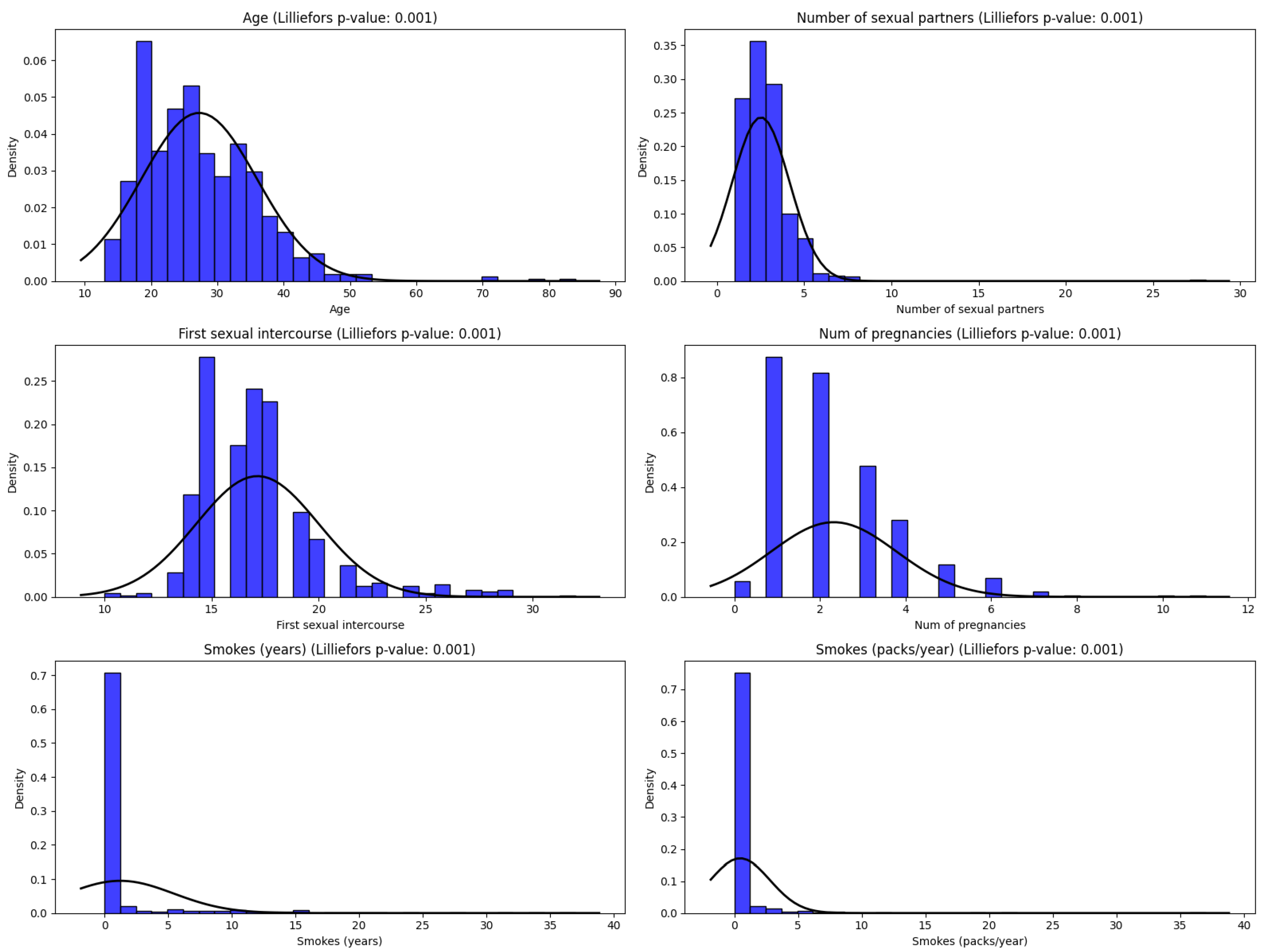
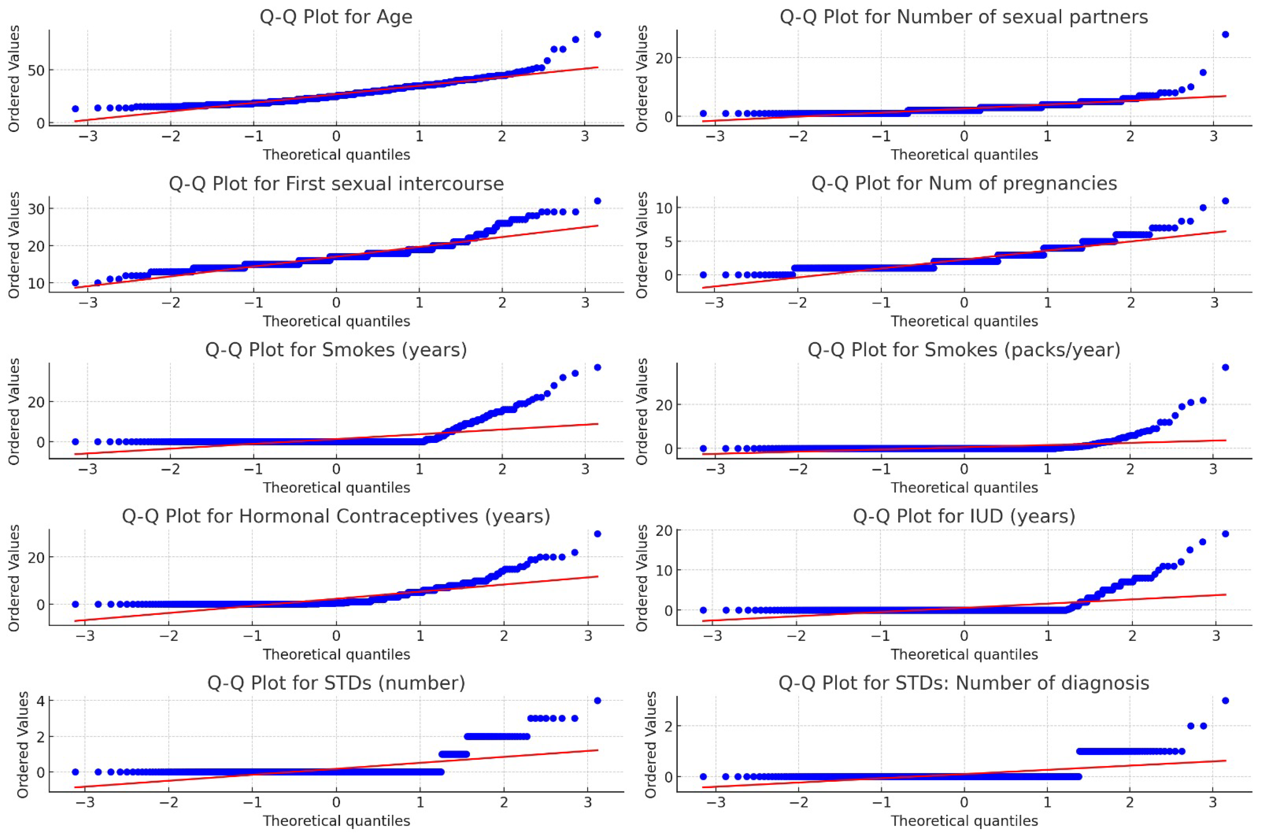
Figure 1. Schematic illustration of the performed research.
Applsci 14 10085 g001
Figure 2. Lilliefors normality test results and visual representation for normality validation.
Applsci 14 10085 g002
Figure 3. A visual approach using Q-Q plots for normality distribution validation.
Applsci 14 10085 g003
Figure 4. ROC-AUC curve with LR before (right) and after (left) oversampling.
Applsci 14 10085 g004
Table 1. Summary statistics of the dataset attributes (integers).
AttributeMinMaxMeanStd DevMedian95% CI Mean
Age138426.828.4925(26.25, 27.39)
Number of sexual partners1282.531.672(2.41, 2.64)
First sexual intercourse103216.992.8017(16.81, 17.18)
Number of pregnancies0112.281.452(2.18, 2.38)
Smokes (years)0371.224.090(0.94, 1.50)
Smokes (packs/year)0370.452.230(0.30, 0.60)
Hormonal contraceptives (years)0302.263.760.5(1.99, 2.53)
IUD (years)0190.511.940(0.37, 0.65)
STDs (number)040.180.560(0.14, 0.22)
STDs: number of diagnoses030.090.300(0.07, 0.11)
Table 2. Performance results of ML models (before applying sampling techniques).
Metric/SamplingKNN2KNN3bLRRF
Accuracy93.1291.5392.5995.76
Ba Accuracy53.5752.7150.0071.42
Precision (Mac;Wght)96.54;93.5958.98;87.9346.29;85.7397.81;95.95
Recall (Mac;Wght)53.57;93.1252.71;91.5350.00;92.5971.42;95.76
MajClass10098.28100100
MinClass7.147.14042.85
F1-Score (Mac;Wght)54.87;90.2653.33;89.3048.07;89.0378.88;94.96
ROC_AUC0.610.630.710.99
Table 3. Performance results of KNN2 (after applying oversampling techniques).
Metric/SamplingSMOTESVM SMOTEBorderline SMOTEADASYN
Accuracy88.3591.0190.4787.83
Ba Accuracy60.8565.5768.5760.57
Precision (Mac;Wght)59.60;89.0966.67;90.7066.43;91.0858.85;87.83
Recall (Mac;Wght)60.85;88.3565.57;91.0068.57;90.4760.57;87.83
MajClass93.1495.4394.2992.57
MinClass28.5735.7142.8628.57
F1 Score (Mac;Wght)60.17;88.7166.09;90.8567.41;90.7659.58;88.36
ROC_AUC0.720.740.740.72
Note: Bolded values indicate significant performance for a metric.
Table 4. Performance results of KNN2 (after applying undersampling techniques).
Metric/SamplingCNNTLAll-KNNRENNENNNCRNM1IHT
Accuracy93.6592.5987.3087.3087.3090.4775.6645.50
Ba Accuracy60.4253.2850.4250.4250.4255.4277.0064.00
Precision (Mac;Wght)84.52;92.6471.52;89.8550.49;86.4050.49;86.4050.49;86.4059.18;88.3059.07;92.0453.99;90.94
Recall (Mac;Wght)60.42;93.6553.28;92.5950.42;87.3050.42;87.3050.42;87.3055.42;90.4777.00;75.6664.00;45.50
MajClass99.4399.4393.7193.7193.7196.5775.4342.29
MinClass21.437.147.147.147.1414.2978.5785.71
F1 Score (Mac;Wght)65.00;91.9754.31;89.9350.43;86.8450.43;86.8450.43;86.8456.56;89.2558.75;81.2438.93;55.99
ROC_AUC0.700.610.610.620.620.630.800.65
Note: Bolded values indicate significant performance for a metric.
Table 5. Performance Results of KNN3 (after applying undersampling techniques).
Metric/SamplingCNNTLAll-KNNRENNENNNCRNM1IHT
Accuracy90.4791.5386.2486.2487.3088.3569.8443.91
Ba Accuracy68.5752.7149.8549.8550.4254.2877.1463.14
Precision (Mac;Wght)66.43;91.0858.98;87.9349.85;86.2449.85;86.2450.49;86.4054.94;87.5458.13;92.4053.80;90.82
Recall (Mac;Wght)68.57;90.4752.71;91.5349.85;86.2449.85;86.2450.42;87.3054.28;88.3577.14;69.8463.14;43.91
MajClass94.2998.2992.5792.5793.7194.2968.5740.57
MinClass42.867.147.147.147.1414.2985.7185.71
F1 Score (Mac;Wght)67.41;90.7653.33;89.3049.85;86.2449.85;86.2450.43;86.8454.56;87.9455.21;77.0137.85;54.38
ROC_AUC0.670.630.600.600.610.620.790.64
Note: Bolded values indicate significant performance for a metric.
Table 6. Performance results of bLR (after applying oversampling techniques).
Metric/SamplingSMOTESVM SMOTEBorderline SMOTEADASYN
Accuracy86.7788.3586.7785.18
Ba Accuracy89.5751.0086.2885.42
Precision (Mac;Wght)67.72;94.6650.89;86.5066.49;93.9265.12;93.70
Recall (Mac;Wght)89.57;86.7751.00;88.3586.28;86.7785.42;85.18
MajClass86.8694.2986.8685.14
MinClass92.867.1485.7185.71
F1 Score (Mac;Wght)72.34;89.6650.74;87.1570.69;89.1968.78;88.05
ROC_AUC0.920.870.890.91
Table 7. Performance results of RF (after applying oversampling techniques).
Metric/SamplingSMOTESVM SMOTEBorderline SMOTEADASYN
Accuracy98.4198.4198.4198.41
Ba Accuracy92.5792.5792.5798.41
Precision (Mac;Wght)95.58;98.3795.58;98.3795.58;98.3795.58;98.37
Recall (Mac;Wght)92.57;98.4192.57;98.4192.57;98.4192.57;98.41
MajClass99.4399.4399.4399.43
MinClass85.7185.7185.7185.71
F1 Score (Mac;Wght)94.01;98.3894.01;98.3894.01;98.3894.01;98.38
ROC_AUC0.990.990.990.99
Note: Bolded values indicate significant performance for a metric.
Table 8. Performance results of RF (after applying undersampling techniques).
Metric/SamplingCNNTLAll-KNNRENNENNNCRNM1IHT
Accuracy98.9495.7695.2397.3596.2996.2995.7676.19
Ba Accuracy96.1471.4267.8582.1475.0075.0097.7183.85
Precision (Mac;Wght)96.14;98.9497.81;95.9596.14;98.9498.07;96.4398.07;96.4398.07;96.4381.81;97.3061.02;93.58
Recall (Mac;Wght)96.14;98.9471.42;95.7667.85;95.2382.14;97.3575.00;96.2975.00;96.2997.71;96.4383.85;76.19
MajClass99.4310010010010010095.4374.86
MinClass92.8642.8664.2964.29505010092.86
F1 Score (Mac;Wght)96.14;98.9478.88;94.9675.06;94.1782.35;95.7182.35;95.7182.35;95.7187.71;96.1860.98;81.73
ROC_AUC0.990.991.01.00.990.990.990.95
Note: Bolded values indicate significant performance for a metric.
Disclaimer/Publisher’s Note: The statements, opinions and data contained in all publications are solely those of the individual author(s) and contributor(s) and not of MDPI and/or the editor(s). MDPI and/or the editor(s) disclaim responsibility for any injury to people or property resulting from any ideas, methods, instructions or products referred to in the content.

