Abstract
In multi-objective optimization, standard evolutionary algorithms, such as NSGA-II, are computationally expensive, particularly when handling complex constraints. Constraint evaluations, often the bottleneck, require substantial resources. Pre-trained surrogate models have been used to improve computational efficiency, but they often rely heavily on the model’s accuracy and require large datasets. In this study, we use active learning to accelerate multi-objective optimization. Active learning is a machine learning approach that selects the most informative data points to reduce the computational cost of labeling data. It is employed in this study to reduce the number of constraint evaluations during optimization by dynamically querying new data points only when the model is uncertain. Incorporating machine learning into this framework allows the optimization process to focus on critical areas of the search space adaptively, leveraging predictive models to guide the algorithm. This reduces computational overhead and marks a significant advancement in using machine learning to enhance the efficiency and scalability of multi-objective optimization tasks. This method is applied to six challenging benchmark problems and demonstrates more than a 50% reduction in constraint evaluations, with varying savings across different problems. This adaptive approach significantly enhances the computational efficiency of multi-objective optimization without requiring pre-trained models.
1. Introduction
Multi-objective optimization (MOO) addresses problems where multiple conflicting objectives must be optimized simultaneously. Unlike single-objective optimization, where a single optimal solution is sought, MOO aims to find a set of Pareto-optimal solutions that represent trade-offs among the objectives. Traditional evolutionary algorithms (EAs), such as NSGA-II (Non-dominated Sorting Genetic Algorithm II), are popular for solving such problems due to their robustness and ability to handle complex, high-dimensional search spaces [1]. However, NSGA-II, while effective, does not incorporate machine learning techniques such as active learning, which can dynamically adapt the optimization process based on uncertainty in constraint evaluations. Unlike NSGA-II, our proposed ALMO method integrates active learning to focus computational resources on critical areas, reducing unnecessary evaluations and improving computational efficiency.
MOO algorithms have been extensively applied in engineering for the design and optimization of complex structures. Vo-Duy et al. [2] achieved the multi-objective optimization of laminated composite beam structures where the objective function was to minimize the weight of the whole laminated composite beam and maximize the natural frequency. Lemonge et al. [3] presented multi-objective structural optimization with conflicting objective functions and constraints, such as the natural frequencies of vibration and the load factors concerning the global stability of the structure. In the field of aerospace engineering, MOO has been employed to optimize the aerodynamic performance and structural integrity of aircraft components. Kim et al. [4] presented the multi-objective and multidisciplinary design optimization of supersonic fighter wings. Wang et al. [5] described the multi-objective optimization of composite aerospace structures while optimizing both the cost and weight of the structure. Borwankar et al. [6] conducted a multidisciplinary design analysis and optimization of space vehicle structures by integrating structural, thermal, and acoustic analysis to optimize the spacecraft’s overall performance while satisfying multiple design constraints. These diverse applications underscore the significance of MOO in solving complex, real-world engineering problems where multiple, often conflicting, criteria must be considered simultaneously.
However, the aforementioned traditional algorithms are often computationally intensive, particularly when faced with complex constraints that necessitate extensive evaluations. The computational expense of MOO arises primarily from the need to evaluate the objective and constraint functions repeatedly across numerous candidate solutions. This is especially challenging in engineering and scientific applications when complex constraints require evaluations that are both time-consuming and resource-demanding. In many engineering applications, such as structural, aerospace, and civil engineering, these evaluations often involve expensive simulations or detailed analyses. One such method commonly used in these fields is the Finite Element Method (FEM), which is computationally expensive. The FEM is widely used in structural optimization to analyze stress, deformation, and other factors under various load conditions, and optimization using FEM can take hours or even days depending on the complexity of the model [7]. In aerospace engineering, MOO frequently deals with aerodynamic shape optimization when the evaluations involve high-fidelity Computational Fluid Dynamics (CFD) simulations. These simulations are also computationally heavy. Furthermore, thermal analysis, required for optimizing the thermal properties of aerospace materials and systems, also significantly adds to the computational cost [8].
To mitigate these challenges, surrogate models have been employed to approximate these expensive evaluations, thereby reducing the overall computational burden [9]. Surrogates, such as response surface models or Kriging models [10], can significantly expedite the optimization process by substituting costly evaluations with less expensive predictions [11]. Sunny et al. [12] presented an artificial neural network residual kriging-based surrogate model for the shape and size optimization of a stiffened panel. Datta and Regis [13] used a surrogate-assisted evolution strategy for constrained multi-objective optimization. Their approach used cubic Radial Basis Function (RBF) surrogate models to assist the optimization by predicting the objective and constraint function values. Lv et al. [14] created a surrogate-assisted particle swarm optimization algorithm for expensive multi-objective optimization. Nik et al. [15] examined the surrogate-based multi-objective optimization of the stiffness and buckling load of a composite laminate plate with curvilinear fiber paths. Jun and Kapania [16,17] developed a deep-learning-based surrogate model that can provide the optimum topologies of 2D and 3D structures.
Despite their advantages, surrogate models require substantial initial training data to achieve high accuracy, and their performance can degrade in large, complex design spaces characterized by numerous local optima [15]. Moreover, the effectiveness of surrogate-based approaches is highly dependent on the quality of the model, which can vary significantly across different regions of the search space. Consequently, there remains a need for more adaptive and efficient methods to improve the computational efficiency of MOO. Wang et al. [18] presented an adaptive response surface method (ARSM) for improving the global optimization of computation-intensive design problems. Steenackers et al. [19] described the development of an adaptive response surface method for the optimization of computationally expensive problems. Their surrogate model is adapted and improved during the optimization and is not trained from a pre-defined number of design experiments. Active learning, a sub-domain of machine learning, offers a promising alternative to traditional surrogate-based approaches. It is an adaptive machine learning technique that incrementally improves a machine learning model by selectively querying the most informative data points. This approach dynamically updates the surrogate model based on the model’s uncertainty, rather than relying on a static, pre-trained model. Wang et al. [20] presented committee-based active learning for the surrogate-assisted particle swarm optimization of computationally expensive problems. Singh and Kapania [21] effectively used active learning in single-objective optimization problems to reduce the number of expensive evaluations by focusing on uncertain regions of the search space.
In this study, we apply active learning to multi-objective optimization problems. Our approach integrates active learning into the MOO framework to adaptively refine the surrogate model during optimization. By querying new data points only when the model is uncertain, we aim to reduce the number of constraint evaluations and enhance the computational efficiency of MOO algorithms. Uncertainty is quantified by calculating the difference in the predicted probabilities from the active learner, which we refer to as the confidence parameter. This parameter helps identify areas where the model is less certain, guiding the selection of new data points. Section 2 presents the details of the methodology of the proposed approach. Section 3 shows the application of the approach to different benchmark constrained optimization problems. The results demonstrate more than 50% reductions in constraint evaluations while maintaining high solution quality. The results of our case studies align well with previous research, particularly in terms of achieving competitive Inverted Generational Distance (IGD) values and maintaining solution quality. A key differentiator of our work is the significant computational savings achieved by reducing constraint evaluations through active learning during the optimization process, a method that has not been extensively explored in prior studies. This underscores the efficiency of ALMO in addressing the computational cost of constrained optimization while maintaining solution accuracy.
2. Methodology
This section presents the methodology of the proposed approach, which is to use active learning for multi-objective optimization to improve constrained evolutionary algorithms. Initially, a brief description of the multi-objective constrained optimization problem is shown. Later, the newly proposed approach of using active learning for improving the optimization is presented.
2.1. Multi-Objective Constrained Optimization
A multi-objective constrained optimization problem can be formulated as
where and are the multiple objective functions, are k constraints, and is the number of design variables. In this problem, there is no single optimal solution, but rather a set of Pareto-optimal solutions representing trade-offs between conflicting objectives. A solution is Pareto-optimal if no objective can be improved without degrading at least one other objective.
2.1.1. NSGA-II for Multi-Objective Optimization
In the present work, the Non-dominated Sorting Genetic Algorithm II (NSGA-II) is employed to solve the multi-objective constrained optimization problem. NSGA-II [1] is widely used for its ability to maintain diversity in the population while efficiently converging to the Pareto front. The key components of NSGA-II are non-dominated sorting and a crowding distance. Non-dominated sorting categorizes the population into several fronts based on Pareto dominance, where each front consists of solutions that are not dominated by any other in the population. The crowding distance helps to maintain a diverse set of solutions by calculating the density of solutions around each individual, ensuring that the population does not converge prematurely to a narrow region of the search space.
At the start of the optimization, a population of individuals is initialized randomly. Each individual represents a potential solution in the design space. The objective functions and constraints are evaluated for each individual. If any individual violates the constraints, it is discarded, ensuring that feasible solutions are prioritized during selection.
NSGA-II uses elitism by combining the parent and offspring populations from each generation, allowing the best solutions from both to survive. The population is sorted based on non-dominance, and the best individuals are selected. The algorithm also incorporates genetic operations, including recombination and mutation, to create new solutions in the next generation.
During optimization, the offspring undergo recombination and mutation. Feasibility is ensured by discarding infeasible offspring and replacing them with new individuals if necessary. The slection of parents for the next generation is based on non-dominated sorting and the crowding distance.
2.1.2. The Steps of NSGA-II in the Current Work
The implementation of NSGA-II follows the steps mentioned below. Its pseudo-code is mentioned in Algorithm 1.
- Parent Initialization: Initialize parent vectors randomly.
- Evaluation: Evaluate the objective functions and constraints for all parent vectors.
- Constraint Handling: Discard infeasible individuals as needed.
- Offspring Generation: Apply recombination and mutation to generate offspring.
- Evaluation: Evaluate the objective functions and constraints for offspring.
- Non-dominated Sorting: Rank all individuals (parents and offspring) based on Pareto dominance.
- Crowding Distance Calculation: Maintain diversity by calculating the crowding distance for each individual.
- Parent Selection: Select the top μ individuals based on non-dominance and the crowding distance for the next generation.
- Convergence Check: Continue until the convergence criteria, such as a stable Pareto front, are met or the maximum number of generations is created.
The optimization stops when the improvement in the Pareto front becomes negligible over several generations, indicating convergence, or when the maximum number of generations is created.
By incorporating NSGA-II, the proposed method efficiently handles multiple objectives while maintaining a diverse set of feasible solutions. This approach is particularly well suited to problems where trade-offs between conflicting design goals are necessary. The optimization is implemented in Python 3.8.3 using a Python-based library: pymoo Multi-objective Optimization in Python [22]. It is a framework that offers state-of-the-art single- and multi-objective optimization algorithms in Python.
| Algorithm 1 NSGA-II |
|
2.2. Active Learning
Active learning (AL), also known as “query learning” or “optimal experimental design”, is a machine learning approach that selects the most informative data points to reduce the computational cost of labeling data. In the context of multi-objective optimization (MOO), active learning focuses on reducing the number of expensive constraint function evaluations while ensuring accurate approximations of the Pareto front. This is particularly valuable in engineering design problems where each evaluation might involve costly simulations or experiments.
The primary goal of AL is to query only those points where the model exhibits uncertainty, avoiding redundant evaluations and concentrating computational resources on data points that provide the most information. By iteratively querying high-uncertainty points, the model converges more efficiently toward an accurate approximation of the Pareto front.
The active learning process begins with a small set of candidate solutions, for which both objective function values and constraint evaluations are available. Based on this training set, a surrogate model is constructed to approximate the feasibility of the candidate solutions, meaning whether they satisfy the constraints or not. In this work, Random Forests (RFs) are employed as the active learner due to their robustness and ability to model complex non-linear relationships [23]. RFs are an ensemble method that aggregates the predictions of multiple decision trees trained on random subsets of the data, providing reliable uncertainty estimates that guide the query process.
As new points are queried, the surrogate model is retrained on the updated dataset, improving its predictions and enhancing the search for the Pareto front.
The Random Forest model used in this study is specifically designed to perform binary classification for feasibility determination while predicting whether a candidate solution satisfies the constraints or not. This binary classification ensures that only feasible solutions are considered for Pareto front approximation.
Uncertainty Quantification for Binary Classification
The uncertainty in the active learning process is driven by the model’s ability to predict whether a candidate solution is feasible, i.e., satisfies the constraints. For each candidate solution, the Random Forest classifier provides a probability distribution over the two classes: feasible (0) and infeasible (1). The uncertainty of a given design point x can be expressed as
The certainty of the model’s prediction is quantified using a confidence parameter , which measures the difference between the predicted probabilities of the two classes:
If the confidence is below a predefined threshold , the model considers the prediction uncertain and queries the true feasibility of the candidate solution. A higher threshold will result in more queries, whereas a lower value will reduce the number of queries but could compromise the accuracy of the predictions. In this study, the balance between exploration and exploitation is controlled by adjusting and the number of trees in the Random Forest, .
By dynamically selecting uncertain points for evaluation, this active learning approach minimizes the number of expensive objective function evaluations while maintaining the diversity and accuracy of the solutions on the Pareto front.
An illustrative example is presented to demonstrate the application of the active learning framework. In this case, a dataset comprising 800 instances, equally divided into two classes, is used, as shown in Figure 1. The active learner is first trained on a small subset of these instances. As the learning process progresses, the model selectively queries the points where it is uncertain, allowing it to improve its accuracy without needing to train over the entire dataset. This process highlights the efficiency of active learning in reducing the overall computational effort while maintaining high predictive performance. Initially, a random subset of 50 instances was selected for training the active learner, which was constructed using a Random Forest classifier with 100 estimators, as shown in Figure 2. The initial performance of the learner across the entire dataset yields an accuracy of 80.6%. At this stage, the learner is tasked with querying data points where its confidence is less than 0.6.
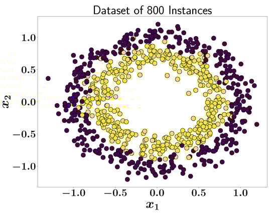
Figure 1.
A dataset of 800 instances available from scikit-learn [24].
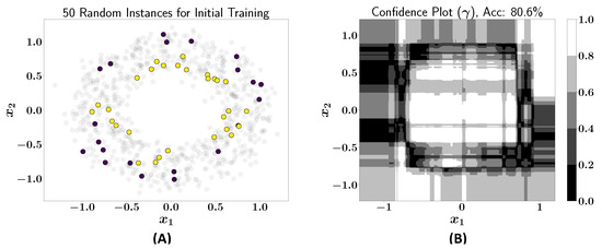
Figure 2.
(A) Fifty labeled instances randomly selected for initial training of active learner; (B) confidence plot after initial training of active learner (accuracy: 80.6%).
Figure 3A shows the 310 queries issued by the active learner. These queries are concentrated in regions where the learner has low confidence, as indicated by the confidence plot in Figure 2B. The newly acquired data points are subsequently added to the training dataset, and the active learner is retrained to improve its classification over the entire dataset. After this, the learner’s accuracy increases significantly to 94.9% across the entire dataset. Figure 3B shows the improvement in the confidence plot in comparison to Figure 2B.
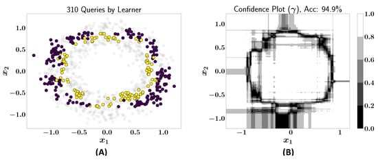
Figure 3.
(A) The 310 queries issued by the learner; (B) confidence plot after including queries in the training dataset (accuracy: 94.9%).
Finally, the active learner is allowed to issue further queries from the remaining dataset. Figure 4A shows 106 additional queries, resulting in a final accuracy of 99% after incorporating the new data into the training set. These queries are concentrated in regions where the learner has low confidence, as indicated by the confidence plot in Figure 3B. Figure 4B shows the improved confidence plot. This example demonstrates that the active learning process can efficiently reach high levels of accuracy without needing to query all available data points.
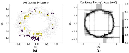
Figure 4.
(A) The 106 queries issued by the learner; (B) confidence plot after including queries in the training dataset (accuracy: 99%).
This case study highlights the efficiency of active learning in boosting model performance by querying selectively, thus avoiding the need to label the entire dataset.
2.3. Active Learning for Multi-Objective Optimization (ALMO)
In this work, we employ an Active Learning-based Multi-Objective Optimization (ALMO) framework to enhance the efficiency of constrained evolutionary optimization algorithms like NSGA-II. By selectively querying expensive constraint evaluations using an active learning model, we can significantly reduce computational costs while maintaining optimization performance. The optimization process proceeds for a total of N generations, where an active learner is trained after the first of these generations.
The ALMO approach is structured as shown in the following steps, while the pseudo-code is shown in Algorithm 2, and the flowchart is shown in Figure 5:
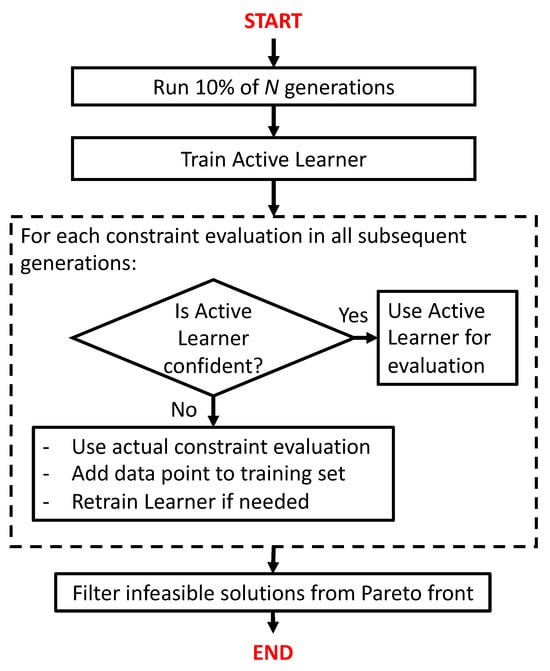
Figure 5.
Flowchart of the constrained optimization procedure using active learning.
- 1.
- Initial Setup: The NSGA-II algorithm begins by initializing a random population of solutions, and true constraint and objective function evaluations are performed for these solutions for the first 10% of the N generations.
- 2.
- Training the Active Learner: After the initial of generations are evaluated, the active learner (a Random Forest classifier) is trained on the available data from these early generations. This learner is then used to perform a binary classification by predicting the feasibility of new solutions in the subsequent generations.
- 3.
- Prediction of Feasibility: During the remaining generations, the active learner predicts the feasibility of the offspring solutions generated by the NSGA-II algorithm. If the learner’s confidence in the feasibility prediction exceeds a defined threshold , the candidate solution is accepted or discarded based on the prediction alone, bypassing the expensive constraint evaluation.
- 4.
- Selective Constraint Evaluation: If the confidence score of the learner falls below , the true constraint function is queried for that solution. These newly evaluated solutions are collected, and the active learner is re-trained once we have m new queries. In this study, we set , where is the population size, ensuring periodic updates while maintaining computational efficiency.
- 5.
- Offspring Selection and Evolution: Feasible offspring, along with selected parents, are carried forward to the next generation following NSGA-II’s selection procedure, which is based on non-dominated sorting and crowding distance metrics. This process continues for the remaining generations.
- 6.
- Final Pareto-front Solution: Once the optimization is complete, the final Pareto-front solutions are evaluated using true constraint functions to ensure their feasibility, while the infeasible solutions are discarded.
| Algorithm 2 ALMO: active learning for multi-objective optimization |
|
This ALMO framework significantly reduces the number of expensive constraint evaluations, particularly in the later stages of the optimization process when the active learner has become more confident in comparison to at the beginning of the optimization. By training the learner after the initial 10% of generations have been evaluated, we ensure that it has enough data to make accurate predictions while maintaining computational efficiency. In experiments with benchmark problems, we observed more than 50% savings in constraint evaluations, depending on the problem’s complexity, the values of , and the number of estimators () in the Random Forest classifier.
The experimental setup also revealed that the ALMO approach retains a high degree of accuracy, as measured by Inverted Generational Distance (IGD), while achieving significant reductions in the total number of function evaluations compared to the total number of evaluations required to conduct the optimization without the use of active learning. For comparison purposes, the solutions obtained using NSGA-II without the use of active learning were employed as the true Pareto front. The IGD measures the proximity of the approximated Pareto front to the true Pareto front. It is calculated as the average Euclidean distance from each point on the true Pareto front to its nearest point on the approximated front:
where is the reference Pareto front, Q is the approximated front, and is the Euclidean distance. Low IGD values indicate that the solutions generated closely match the reference optimal solutions’ objective functions. Since optimal objective function values are achieved from corresponding optimal design variable values, it follows that the design variables are also close to the reference results. Thus, low IGD values provide a strong indication that both the objective and design variable values are comparable.
3. Application and Results
This section presents the application of the ALMO framework introduced in Section 2 to six well-known benchmark problems: OSY [25], BNH [26], TNK [27], MW1, MW9, and MW12 [28]. The active learner in ALMO uses a Random Forest model as its estimator throughout these case studies. In Section 3.1, Section 3.2, Section 3.3, Section 3.4, Section 3.5 and Section 3.6, we evaluate ALMO’s performance on each benchmark problem to demonstrate two key aspects: (1) ALMO consistently finds the near-optimal solutions referenced in the literature and (2) it significantly reduces the number of constraint evaluations compared to traditional constrained evolutionary algorithms, such as those discussed in the benchmark papers cited. The constraint and objective function plots of the benchmark problems used in this study are found in their respective original papers. These plots have been extensively studied and documented in the literature, so they are not reproduced here. The optimization is implemented in Python using a Python-based library: pymoo Multi-objective Optimization in Python [22]. In all the case studies, a population size of 300 was considered, and the NSGA-II algorithm was used to conduct optimization for 600 generations. Initially, NSGA-II is applied to all the problems without any active learning integration to ensure the correctness of the setup and to establish a baseline for calculating the IGD. We then implement the ALMO framework to present the benefits as compared to the baseline found using NSGA-II. Later, we investigate the impact of varying and on the percentage of infeasible solutions present in the final Pareto front. Specifically, is tested at values of 50, 100, 150, and 200, while ranges from 0.6 to 0.9. The reported infeasibility rates reflect how effectively the ALMO framework manages constraints during optimization. Lower infeasibility rates indicate that the active learner successfully identifies feasible regions in the search space. A higher infeasibility rate suggests that the problem’s constraints are more challenging for the learner to predict accurately. However, the consistently low infeasibility rates across most configurations demonstrate that ALMO maintains feasibility effectively while minimizing constraint violations, showcasing its robustness in handling complex multi-objective problems. Finally, we analyze how the savings in constraint evaluations evolve throughout the optimization process.
MW1, MW9, and MW12 are selected to represent a range of problem complexities. MW1 is relatively easier, allowing us to demonstrate ALMO’s effectiveness when constraints are manageable, while MW9 and MW12 are more challenging, highlighting the framework’s performance under more complex conditions. This selection provides a balanced view of ALMO’s capabilities across varying problem difficulties without a redundant analysis of the entire MW suite. By focusing on these specific problems, we show how ALMO handles both simpler and more difficult optimization challenges.
3.1. Case Study I: The OSY Problem
In this case study, we apply the ALMO approach to the OSY problem, originally introduced by A. Osyczka and S. Kundu [25]. The OSY problem is a widely used benchmark for multi-objective optimization, characterized by non-linear constraints and a relatively complex solution space. The problem is formulated as follows:
and subject to the following six constraints:
with the variable bounds
To benchmark the ALMO’s performance, we apply the NSGA-II algorithm without active learning to establish a baseline for comparing the benefits of the ALMO framework, as shown in Figure 6.
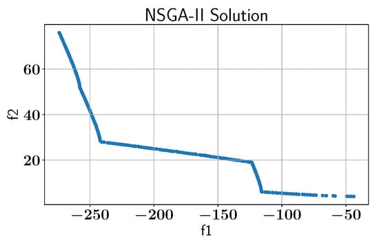
Figure 6.
Case Study I: Pareto-front solution found by NSGA-II without AL using pymoo library.
Subsequently, the ALMO approach is employed to solve the OSY problem, using two configurations of and , as shown in all feasible Pareto-front solutions in Figure 7. In the first scenario, is set to 100 and is set to 0.7, which results in an IGD of 0.002. In the second configuration, is increased to 200 while is set to 0.9, and the IGD remains at 0.002, indicating that both settings provide optimal solutions with low IGD values. However, the configurations show different performances in constraint handling, as discussed below.
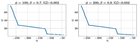
Figure 7.
Case Study I: Pareto-front solution found using ALMO and two different configurations.
We next analyze the percentage of infeasible solutions present in the final Pareto fronts across various configurations of and , as shown in Figure 8A. For , the percentage of infeasible solutions remains greater than or equal to 5% for all the values of . When , the percentage of infeasible solutions is consistently less than 5% for , while for , the number of infeasible solutions drops to around 1%. It can be seen that as the value is increased, there are, overall, fewer infeasible solutions in the final Pareto front.
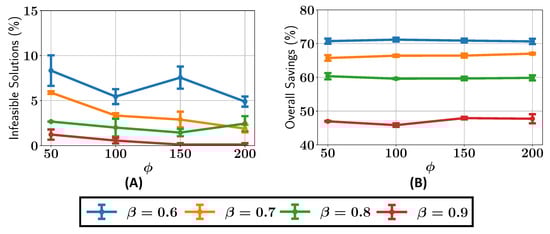
Figure 8.
Case study I: (A) percentage of infeasible solutions found in the optimal Pareto front; (B) overall savings in constraint evaluations in optimizations with different values of and .
The ALMO approach also demonstrates significant savings in constraint evaluations, as shown in Figure 8B. The savings decrease steadily with higher values, starting at around 70% for , rising to 65% for , 60% for , and reaching approximately 45% for . However, due to the inherent randomness in the population generated by the algorithm, some variability in the results is expected, leading to minor fluctuations in the observed savings and percentage of infeasible solutions.
Lastly, the savings in constraint evaluations are examined across different optimization intervals. As the optimization progresses, the savings increase, demonstrating that ALMO becomes more effective at reducing the number of evaluations as the algorithm becomes more confident in identifying feasible regions. Figure 9 shows the percentage savings over the optimization interval, with ALMO achieving around 20% savings in the early stages, which increases to about 60% and 75% as the optimization proceeds. This trend further confirms the ability of ALMO to enhance efficiency in multi-objective optimization, particularly in later stages when the algorithm’s predictions are more reliable.
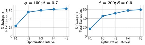
Figure 9.
Case study I: percentage of savings in constraint evaluations in different optimization intervals using ALMO with two different configurations.
3.2. Case Study II: The BNH Problem
For this case study, we apply the ALMO approach to solve the BNH problem, which is a well-known benchmark problem in multi-objective constrained optimization. The BNH problem was originally introduced by To Thanh Binh and Ulrich Korn [26] and involves two objective functions and two non-linear constraints. The mathematical formulation of the BNH problem is as follows:
subject to the following two constraints:
where the decision variables and are bounded as
Figure 10 shows the solution for the BNH problem implemented using NSGA-II and the pymoo Python library to establish a baseline for comparing the benefits of the ALMO framework.
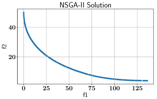
Figure 10.
Case study II: Pareto-front solution found by NSGA-II without AL using pymoo library.
Subsequently, the ALMO approach is applied with two configurations of and . In the first configuration, is set to 100 and is set to 0.7, resulting in an IGD of 0.002. The second configuration involves setting to 200 and to 0.9, and the IGD remains at 0.002. Figure 11 illustrates all feasible Pareto fronts obtained for both configurations, which indicates that both settings produce optimal solutions with minimal IGD values. This consistent performance suggests that the BNH problem is well handled by the ALMO framework across different parameter settings.

Figure 11.
Case study II: Pareto-front solution found using ALMO and two different configurations.
We then examine the percentage of infeasible solutions present in the final Pareto fronts for various values of and , as shown in Figure 12A. Interestingly, for all the configurations, the percentage of infeasible solutions is 0%. This is indicative of the fact that the BNH problem’s feasible space is relatively easier for the learner to grasp compared to other problems like the OSY (Section 3.1) and due to the fact that neither constraint defined in the problem renders any solution from the unconstrained Pareto-optimal front infeasible. Therefore, the constraints might not significantly increase the difficulty of solving this problem. The absence of infeasible solutions highlights the robustness of the ALMO in maintaining feasibility while optimizing the objectives.
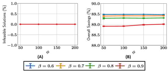
Figure 12.
Case study II: (A) percentage of infeasible solutions found in the optimal Pareto front; (B) overall savings in constraint evaluations in optimizations with different values of and .
Furthermore, the ALMO approach exhibits substantial savings in constraint evaluations, as shown in Figure 12B. For all tested configurations, the overall savings in the constraint evaluations remain close to 89%. This indicates that the ALMO framework is particularly effective in reducing the computational cost for the BNH problem, where the feasible region is well-defined and can be efficiently exploited by the learner.
Lastly, the constraint evaluation savings are analyzed across different optimization intervals, revealing that ALMO becomes increasingly efficient as the optimization progresses, as shown in Figure 13. In the first interval of the optimization process, ALMO achieves around 50% savings, which increases to approximately 99% as the optimization proceeds. This trend reflects the growing confidence of the active learner in identifying feasible and optimal regions of the search space as the evolutionary process unfolds.
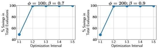
Figure 13.
Case study II: percentage of savings in constraint evaluations in different optimization intervals using ALMO with two different configurations.
3.3. Case Study III: Then TNK Problem
In this section, we apply the ALMO approach to the well-known TNK problem introduced by M. Tanaka et al. [27]. The TNK problem is a constrained bi-objective optimization problem notable for its non-linear and nonconvex constraints, making it a challenging test case for multi-objective optimization algorithms. The TNK problem is formulated as follows:
subject to the constraints
with the variable bounds
The TNK problem’s nonconvex constraints pose a significant challenge for traditional optimization algorithms. The results obtained using the NSGA-II implementation are shown in Figure 14 to establish a baseline for comparing the benefits of ALMO framework.

Figure 14.
Case study III: Pareto-front solution found by NSGA-II without AL using pymoo library.
Next, the ALMO approach is applied using two different configurations of and . In the first case, is set to 100 and is set to 0.7, yielding an IGD of 0.002. In the second configuration, is increased to 200 and is set to 0.9, which results in the IGD being 0.001. Figure 15 displays all feasible Pareto fronts for both configurations, demonstrating that higher values of and generally result in a better IGD performance.
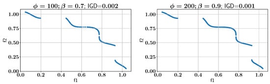
Figure 15.
Case study III: Pareto-front solution found using ALMO and two different configurations.
Figure 16A shows that for , approximately 15% of the candidate solutions are infeasible, which decreases significantly to around 1% for . This pattern suggests that higher values of result in better constraint handling, reducing the number of infeasible solutions in the final Pareto front. Compared to the OSY problem (Section 3.1), the TNK problem results in more infeasible solutions, suggesting that it is relatively more difficult for the learner to identify feasible regions in the search space.
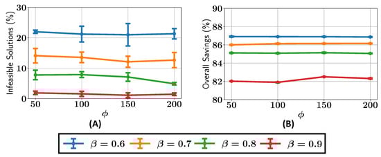
Figure 16.
Case study III: (A) percentage of infeasible solutions found in the optimal Pareto front; (B) overall savings in constraint evaluations in the optimization with different values of and .
The ALMO approach also demonstrates substantial savings in the number of constraint evaluations required to solve the TNK problem, as shown in Figure 16B. For , the approach achieves an impressive 86% saving in constraint evaluations, while for , the savings are around 82%. These savings highlight the efficiency of ALMO in handling optimization problems with fewer constraint violations. Also, it should be noted that due to the inherent randomness in the population generated by the algorithm, some variability in the results is expected, leading to minor fluctuations in the observed savings and percentage of infeasible solutions.
Figure 17 illustrates the percentage of constraint evaluations saved across different optimization intervals. During the initial 20% of the optimization process, ALMO achieves around 40% savings, which steadily increase to approximately 90% by the final interval. This increase in savings as the optimization proceeds indicates that the ALMO approach becomes more confident in its predictions over time, resulting in greater computational efficiency during the later stages of the optimization as the Pareto front calculation progresses.
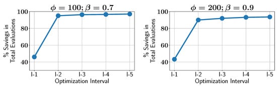
Figure 17.
Case study III: percentage of savings in constraint evaluations in different optimization intervals using ALMO in two different configurations.
3.4. Case Study IV: The MW1 Problem
In this section, we demonstrate the application of the ALMO approach for solving the MW1 problem introduced by Zhongwei Ma and Yong Wang in [28]. The problem has fifteen design variables, the following two objective functions, and one constraint. The mathematical formulation of the MW1 problem is as follows:
where the function is defined as
subject to the following constraint:
where the decision variables to are bounded as
First, we apply the NSGA-II algorithm without any active learning to establish a baseline for comparing the benefits of the ALMO framework and to ensure that the solutions match the results presented in the literature [22,28], as shown in Figure 18.
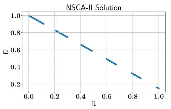
Figure 18.
Case study IV: Pareto-front solution found by NSGA-II without AL using pymoo library.
We then apply the ALMO approach to the MW1 problem using two different configurations of the hyperparameters and . The first configuration uses and and the second configuration uses and . Both configurations achieve a similar IGD value of 0.001. Figure 19 shows all feasible Pareto fronts obtained from these two ALMO configurations. As demonstrated, both approaches yield near-optimal solutions, closely aligned with the true Pareto front.
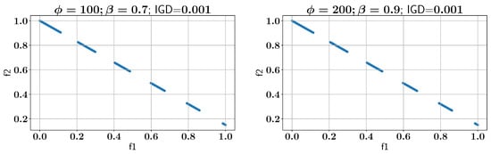
Figure 19.
Case study IV: Pareto-front solution found using ALMO and two different configurations.
Next, we analyzed the effect of different values of and on the percentage of infeasible solutions in the final Pareto front. Figure 20A presents the results of this analysis, where was varied along with . The findings show that at , approximately 7.5% of the solutions were infeasible. As increased to 0.7, the infeasibility rate decreased to around 5%. Further increases in led to a reduction of approximately 2.5% at , and, finally, the rate dropped to about 1% when was increased to 0.9.
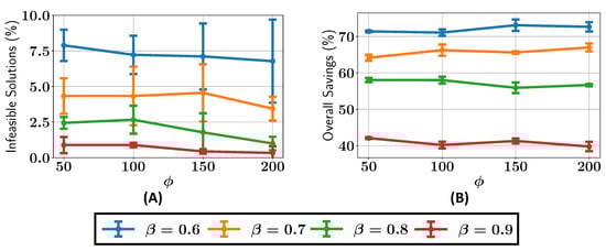
Figure 20.
Case study IV: (A) percentage of infeasible solutions found in the optimal Pareto front; (B) overall savings in constraint evaluations in the optimization with different values of and .
Moreover, Figure 20B presents the overall savings in constraint evaluations across different combinations of and . With , we achieved around a 65% saving in constraint evaluations, while with , the savings were approximately 40%. These savings indicate that the ALMO approach effectively reduces the computational burden by minimizing the number of constraint evaluations required to find feasible solutions.
Finally, we investigate how the percentage savings in constraint evaluations increase over the optimization intervals. Figure 21 shows that as the optimization proceeds, the percentage savings increase. During the initial stages of the optimization, the savings are around 30% for and . However, as the optimization progresses and the active learner becomes more confident, the savings increase significantly, reaching about 80% in the final stages. A similar trend can be seen for the ALMO configuration with and , where the savings per interval increase from about 20% to 50%.
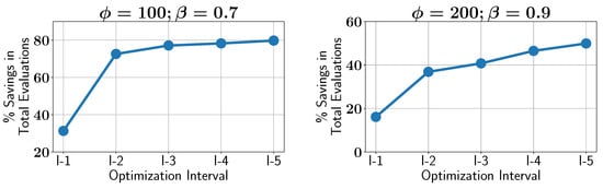
Figure 21.
Case study IV: percentage of savings in constraint evaluations in different optimization intervals using ALMO in two different configurations.
3.5. Case Study V: The MW9 Problem
In this section, we apply the ALMO approach to solving the MW9 problem, which is part of the test suite introduced by Zhongwei Ma and Yong Wang [28]. The MW9 problem is a constrained multi-objective optimization problem that presents a challenging landscape due to its non-linear constraints and multiple objectives. The mathematical formulation of the MW9 problem can be described as follows:
where is defined in Section 3.4. The problem is subject to the following non-linear constraint:
where the decision variables to are bounded as
The MW9 problem is known for its complicated Pareto front and complex constraint region, which together make it an ideal candidate to evaluate the efficiency and accuracy of the ALMO approach. Initially, the NSGA-II algorithm is used without any active learning to establish a baseline for comparing the benefits of the ALMO framework and to ensure the solutions matched those reported in the literature [22,28], as shown in Figure 22.
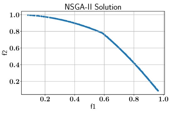
Figure 22.
Case study V: Pareto-front solution found by NSGA-II without AL using pymoo library.
After validating the baseline solution with NSGA-II, the ALMO approach is applied to solve MW9 using different parameter settings for the active learner, as shown in Figure 23. The first experiment involves setting and , resulting in an IGD of 0.013. This is followed by an experiment with and , where the IGD improves to 0.003, demonstrating that increasing both and can lead to a better approximation of all feasible Pareto fronts. Figure 24 shows a Pareto-front solution where is increased from 0.7 to 0.8 while having , and it improves the IGD to 0.004, demonstrating that this optimization problem needs a higher value because of its complex constraint.
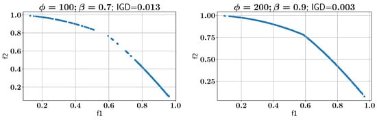
Figure 23.
Case study V: Pareto-front solution found using ALMO and two different configurations.
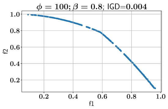
Figure 24.
Case study V: Pareto-front solution found using ALMO.
To further investigate the behavior of the ALMO approach, different combinations of and are tested, as shown in Figure 25A. The results reveal that for , the percentage of infeasible solutions in the final Pareto front remains below 10%, whereas for , the infeasible solutions drop to around 5%. Compared to the MW1 problem discussed in Section 3.4, the percentage of infeasible solutions in MW9 is notably higher. This is likely due to the increased complexity of the MW9 problem, which makes it more difficult for the active learner to accurately predict feasible solutions.
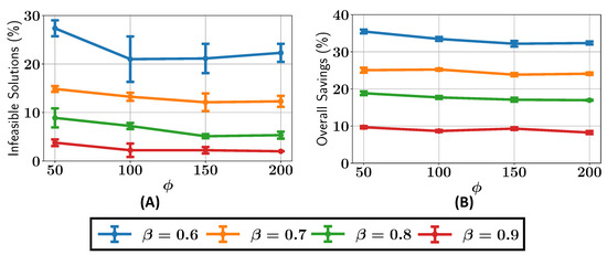
Figure 25.
Case study V: (A) percentage of infeasible solutions found in the optimal Pareto front; (B) overall savings in constraint evaluations in the optimization with different values of and .
In terms of constraint evaluation savings, the results show that with , the ALMO approach achieves approximately 15 to 20% savings, while for , the savings are around 10%, as shown in Figure 25B. These savings are lower than those observed for the MW1 problem, again highlighting the increased difficulty of the MW9 problem for the active learner. Nevertheless, the ALMO approach still demonstrates significant computational savings compared to a traditional NSGA-II run without active learning. There are minor fluctuations in the percentage of feasible solutions and overall savings due to inherent randomness in the population generated by the algorithm.
Finally, the impact of the ALMO approach on constraint evaluation savings over different optimization intervals is studied. As with the MW1 problem, the savings tend to increase as the optimization proceeds, with the active learner becoming more confident in its predictions. Figure 26 illustrates the increasing percentage savings in constraint evaluations across five equal optimization intervals.
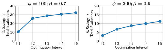
Figure 26.
Case study V: percentage of savings in constraint evaluations in different optimization intervals using ALMO and two different configurations.
3.6. Case Study VI: The MW12 Problem
In this case study, the ALMO approach is applied to the MW12 problem, another constrained multi-objective optimization problem from the test suite introduced by Zhongwei Ma and Yong Wang [28]. The MW12 problem is characterized by its highly complex Pareto front and constraint region, making it one of the most challenging problems in the suite. The mathematical formulation of the MW12 problem is as follows:
where is as defined in Section 3.4. The problem is subject to the following non-linear constraints:
where the decision variables to are bounded as
As with the previous problems, we began by solving MW12 using the NSGA-II algorithm without any active learning to establish a baseline and ensure that the obtained solutions match those reported in the literature [22,28], as shown in Figure 27.
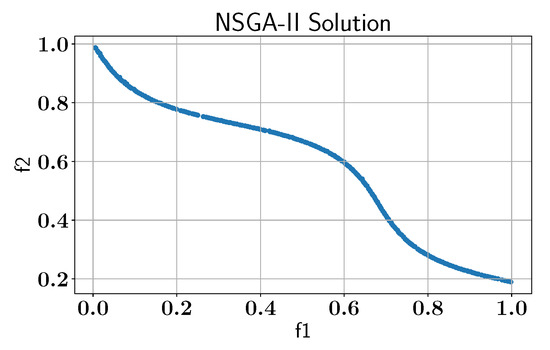
Figure 27.
Case study VI: Pareto-front solution found by NSGA-II without AL using pymoo library.
Once the baseline is established, the ALMO approach is applied to MW12 using two different parameter settings for and . In the first experiment, is set to 100 and is set to 0.7, which results in an IGD of 0.024. In the second experiment, is increased to 200 and is increased to 0.9, and the IGD improves significantly to 0.003. Figure 28 illustrates all feasible Pareto fronts for both parameter settings, demonstrating that the ALMO approach performs better with higher values of and , as also observed in the MW9 case study (Section 3.5). Figure 29 shows the Pareto front for the configuration where is increased to 0.8 from 0.7 while keeping as 100. The IGD of this solution improves to 0.004, demonstrating the need for higher values if the constraints of the problem statement are difficult for the learner to understand.
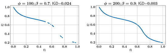
Figure 28.
Case study VI: Pareto-front solution found using ALMO and two different configurations.
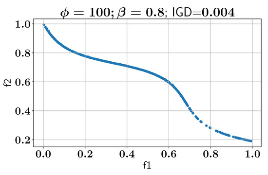
Figure 29.
Case study VI: Pareto-front solution found using ALMO.
Next, the effect of varying and on the percentage of infeasible solutions in the final Pareto front is explored and shown in Figure 30. The results show that with , around 25% of the candidate solutions in the final Pareto front are infeasible, and when , this reduces to about 20%. This drops significantly, to below 5%, when is increased to 0.9. Interestingly, the percentage of infeasible solutions in the MW12 problem is higher than that observed for MW9 (Section 3.5), likely because MW12 presents a more complex and difficult landscape for the active learner to model accurately.
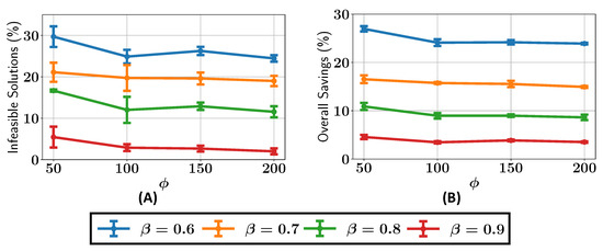
Figure 30.
Case study VI: (A) percentage of infeasible solutions found in the optimal Pareto front; (B) overall savings in constraint evaluations in the optimization with different values of and .
In terms of constraint evaluation savings, the ALMO approach shows more modest savings for the MW12 problem compared to MW9. With , approximately 10% of the constraint evaluations are saved, whereas with , the savings drop to around 5%. The lower savings compared to MW9 suggest that the increased difficulty of MW12 requires more constraint evaluations to ensure feasible solutions, despite its improved IGD values.
Finally, we investigate how the savings in constraint evaluations evolve over the course of the optimization process. Similar to the MW9 problem, the ALMO approach becomes more efficient as the optimization proceeds, achieving greater savings in its later stages. Figure 31 illustrates the percentage savings in constraint evaluations across five equal optimization intervals.
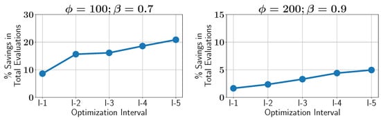
Figure 31.
Case study VI: percentage of savings in constraint evaluations in different optimization intervals using ALMO and two different configurations.
4. Conclusions
In this paper, we introduce the active learning-based multi-objective optimization (ALMO) framework, designed to accelerate constrained evolutionary algorithms like NSGA-II by significantly reducing the number of costly constraint evaluations required. The core of this approach is the integration of an active learner, which dynamically queries new data points only when uncertainty arises. The effectiveness of the ALMO approach is demonstrated through its application to six benchmark problems, where it achieves significant constraint evaluation savings.
A key finding from this study is that the ALMO framework maintains high solution quality, as evidenced by the IGD values, while improving computational efficiency by minimizing unnecessary evaluations. The success of the method relies on tuning parameters such as the learner’s confidence threshold, , and the number of estimators, , for the Random Forest model. Values of above 0.7 are generally found to result in fewer infeasible solutions and higher savings in the constraint evaluations.
We found that while ALMO delivers significant computational savings, the extent of these savings can decrease when more complex constraints require higher values to maintain solution feasibility. This trade-off between feasibility and savings is a potential limitation, as higher values increase the learner’s confidence threshold, potentially requiring more constraint evaluations. However, even in such cases, ALMO still reduces the overall computational burden compared to traditional methods, though the savings may be less pronounced for problems with more challenging constraint landscapes.
In future work, the ALMO framework can be extended in several promising directions. One potential improvement includes the exploration of advanced machine learning techniques, such as ensemble methods or deep learning architectures, to enhance the accuracy and adaptability of the active learner. Additionally, refining uncertainty quantification techniques could improve the querying strategy, leading to more efficient optimization by minimizing unnecessary evaluations. Another promising direction is the application of the ALMO framework to more diverse and complex multi-objective problems, which could further validate its effectiveness and robustness across various domains. Finally, investigating the integration of ALMO with other optimization algorithms may also provide insights into improving its performance in different optimization scenarios.
Author Contributions
Conceptualization, K.S.; Methodology, K.S.; Software, K.S.; Validation, K.S.; Formal analysis, K.S.; Investigation, K.S.; Resources, K.S.; Data curation, K.S.; Writing—original draft, K.S.; Writing—review & editing, R.K.K.; Visualization, K.S.; Supervision, R.K.K. All authors have read and agreed to the published version of the manuscript.
Funding
This research received no external funding.
Institutional Review Board Statement
Not applicable.
Informed Consent Statement
Not applicable.
Data Availability Statement
The original contributions presented in the study are included in the article, further inquiries can be directed to the corresponding author.
Conflicts of Interest
The authors declare no conflicts of interest.
Nomenclature
| k | Number of constraints |
| Number of design variables | |
| Population size | |
| Offspring size | |
| p | Probability of a prediction |
| Confidence parameter | |
| Threshold value for | |
| Number of estimators in the active learner | |
| m | Number of queries collected before re-training the active learner |
| N | Maximum allowed generations for optimization |
References
- Deb, K.; Pratap, A.; Agarwal, S.; Meyarivan, T. A fast and elitist multiobjective genetic algorithm: NSGA-II. IEEE Trans. Evol. Comput. 2002, 6, 182–197. [Google Scholar] [CrossRef]
- Vo-Duy, T.; Duong-Gia, D.; Ho-Huu, V.; Vu-Do, H.; Nguyen-Thoi, T. Multi-objective optimization of laminated composite beam structures using NSGA-II algorithm. Compos. Struct. 2017, 168, 498–509. [Google Scholar] [CrossRef]
- Lemonge, A.C.C.; Carvalho, J.P.G.; Hallak, P.H.; Vargas, D.E.C. Multi-objective truss structural optimization considering natural frequencies of vibration and global stability. Expert Syst. Appl. 2021, 165, 113777. [Google Scholar] [CrossRef]
- Kim, Y.; Jeon, Y.; Lee, D. Multi-objective and multidisciplinary design optimization of supersonic fighter wing. J. Aircr. 2006, 43, 817–824. [Google Scholar] [CrossRef]
- Wang, K.; Kelly, D.; Dutton, S. Multi-objective optimisation of composite aerospace structures. Compos. Struct. 2002, 57, 141–148. [Google Scholar] [CrossRef]
- Borwankar, P.; Kapania, R.K.; Inoyama, D.; Stoumbos, T. Multidisciplinary design analysis and optimization of space vehicle structures. In Proceedings of the AIAA SCITECH 2024 Forum, Orlando, FL, USA, 8–12 January 2024. [Google Scholar]
- Cagnina, L.C.; Esquivel, S.C.; Coello, C.A.C. Solving engineering optimization problems with the simple constrained particle swarm optimizer. Informatica 2008, 32, 319–326. [Google Scholar]
- Voutchkov, I.; Keane, A. Multi-objective Optimization Using Surrogates. In Computational Intelligence in Optimization. Adaptation, Learning, and Optimization; Tenne, Y., Goh, C., Eds.; Springer: Berlin/Heidelberg, Germany, 2010; pp. 155–175. [Google Scholar]
- Wang, Z.; Li, J.; Rangaiah, G.P.; Wu, Z. Machine learning aided multi-objective optimization and multi-criteria decision making: Framework and two applications in chemical engineering. Comput. Chem. Eng. 2022, 165, 107945. [Google Scholar] [CrossRef]
- Tamijani, A.Y.; Mulani, S.B.; Kapania, R.K. A framework combining meshfree analysis and adaptive kriging for optimization of stiffened panels. Struct. Multidiscip. Optim. 2014, 49, 577–594. [Google Scholar] [CrossRef]
- Singh, P.; Couckuyt, I.; Ferranti, F.; Dhaene, T. A constrained multi-objective surrogate-based optimization algorithm. In Proceedings of the 2014 IEEE Congress on Evolutionary Computation (CEC), Beijing, China, 6–11 July 2014. [Google Scholar]
- Sunny, M.R.; Mulani, S.B.; Sanyal, S.; Pant, R.S.; Kapania, R.K. An artificial neural network residual kriging based surrogate model for shape and size optimization of a stiffened panel. In Proceedings of the 54th AIAA/ASME/ASCE/AHS/ASC Structures, Structural Dynamics, and Materials Conference, Boston, MA, USA, 8–11 April 2013. [Google Scholar]
- Datta, R.; Regis, R.G. A surrogate-assisted evolution strategy for constrained multi-objective optimization. Expert Syst. Appl. 2016, 57, 270–284. [Google Scholar] [CrossRef]
- Lv, Z.; Wang, L.; Han, Z.; Zhao, J.; Wang, W. Surrogate-assisted particle swarm optimization algorithm with pareto active learning for expensive multi-objective optimization. IEEE/CAA J. Autom. Sin. 2019, 6, 838–849. [Google Scholar] [CrossRef]
- Nik, M.A.; Fayazbakhsh, K.; Pasini, D.; Lessard, L. Surrogate-based multi-objective optimization of a composite laminate with curvilinear fibers. Compos. Struct. 2012, 94, 2306–2313. [Google Scholar]
- Seo, J.; Kapania, R.K. Topology optimization with advanced CNN using mapped physics-based data. Struct. Multidiscip. Optim. 2023, 66, 21. [Google Scholar] [CrossRef]
- Seo, J.; Kapania, R.K. Development of deep convolutional neural network for structural topology optimization. AIAA J. 2023, 61, 1366–1379. [Google Scholar] [CrossRef]
- Wang, G.G.; Dong, Z.; Aitchison, P. Adaptive response surface method-A global optimization scheme for approximation-based design problems. Eng. Optim. 2001, 33, 707–734. [Google Scholar] [CrossRef]
- Steenackers, G.; Presezniak, F.; Guillaume, P. Development of an adaptive response surface method for optimization of computation-intensive models. Comput. Ind. Eng. 2009, 57, 847–855. [Google Scholar] [CrossRef]
- Wang, H.; Jin, Y.; Doherty, J. Committee-based active learning for surrogate-assisted particle swarm optimization of expensive problems. IEEE Trans. Cybern. 2017, 47, 2664–2677. [Google Scholar] [CrossRef]
- Singh, K.; Kapania, R.K. ALGA: Active learning-based genetic algorithm for accelerating structural optimization. AIAA J. 2021, 59, 330–344. [Google Scholar] [CrossRef]
- Blank, J.; Deb, K. Pymoo: Multi-objective optimization in python. IEEE Access 2020, 8, 89497–89509. [Google Scholar] [CrossRef]
- Breiman, L. Random forests. Mach. Learn. 2001, 45, 5–32. [Google Scholar] [CrossRef]
- Pedregosa, F.; Varoquaux, G.; Gramfort, A.; Michel, V.; Thirion, B.; Grisel, O.; Blondel, M.; Prettenhofer, P.; Weiss, R.; Dubourg, V.; et al. Scikit-learn: Machine learning in python. J. Mach. Learn. Res. 2011, 12, 2825–2830. [Google Scholar]
- Osyczka, A.; Kundu, S. A new method to solve generalized multicriteria optimization problems using the simple genetic algorithm. Struct. Optim. 1995, 10, 94–99. [Google Scholar] [CrossRef]
- Binh, T.T.; Korn, U. MOBES: A multiobjective evolution strategy for constrained optimization problems. In Proceedings of the Third International Conference on Genetic Algorithms (Mendel 97), Brno, Czech Republic, 25–27 June 1997. [Google Scholar]
- Tanaka, M.; Watanabe, H.; Furukawa, Y.; Tanino, T. GA-based decision support system for multicriteria optimization. In Proceedings of the 1995 IEEE International Conference on Systems, Man and Cybernetics. Intelligent Systems for the 21st Century, Vancouver, BC, Canada, 22–25 October 1995; Volume 2, pp. 1556–1561. [Google Scholar]
- Ma, Z.; Wang, Y. Evolutionary constrained multiobjective optimization: Test suite construction and performance comparisons. IEEE Trans. Evol. Comput. 2019, 23, 972–986. [Google Scholar] [CrossRef]
Disclaimer/Publisher’s Note: The statements, opinions and data contained in all publications are solely those of the individual author(s) and contributor(s) and not of MDPI and/or the editor(s). MDPI and/or the editor(s) disclaim responsibility for any injury to people or property resulting from any ideas, methods, instructions or products referred to in the content. |
© 2024 by the authors. Licensee MDPI, Basel, Switzerland. This article is an open access article distributed under the terms and conditions of the Creative Commons Attribution (CC BY) license (https://creativecommons.org/licenses/by/4.0/).