Spectrogram-Based Arrhythmia Classification Using Three-Channel Deep Learning Model with Feature Fusion

Abstract

This paper introduces a novel deep learning model for ECG signal classification using feature fusion. The proposed methodology transforms the ECG time series into a spectrogram image using a short-time Fourier transform (STFT). This spectrogram is further processed to generate a histogram of oriented gradients (HOG) and local binary pattern (LBP) features. Three separate 2D convolutional neural networks (CNNs) then analyze these three image representations in parallel. To enhance performance, the extracted features are concatenated before feeding them into a gated recurrent unit (GRU) model. The proposed approach is extensively evaluated on two ECG datasets (MIT-BIH + BIDMC and MIT-BIH) with three and five classes, respectively. The experimental results demonstrate that the proposed approach achieves superior classification accuracy compared to existing algorithms in the literature. This suggests that the model has the potential to be a valuable tool for accurate ECG signal classification, aiding in the diagnosis and treatment of various cardiovascular disorders.

1. Introduction

Arrhythmia affects heart rhythm, characterized by an irregular heartbeat that can be either faster or slower than usual. Electrocardiogram (ECG) is the primary diagnostic tool used to detect such abnormalities, but detecting and classifying arrhythmias can be challenging due to the nature of ECG signals. Automated arrhythmia analysis could provide a faster and more accurate solution to these challenges [1,2,3,4,5,6,7]. Several studies have been conducted to diagnose ECGs using signal processing, machine learning, and deep learning techniques. For example, Kiranyaz et al. [8] developed a patient-specific electrocardiogram classification and monitoring system using an adaptive implementation of 1D convolutional neural networks (CNNs). By training a separate CNN for each patient, patient-specific features were extracted, leading to increased classification performance. The researchers in [9] used the n-beat-score map (n-BSM), a 2D ECG representation, in an adversarial framework to improve arrhythmia classification. They trained a beat classifier to generate a patient-independent n-BSM (PI-BSM), reducing the impact of patient-specific features. Acharya et al. [10] used a nine-layer deep convolutional neural network (CNN) to automatically classify five different heartbeat arrhythmias in the MIT-BIH arrhythmia dataset. After applying a lowpass filter to the original data, they performed experiments on both noisy and noise-free data. In another study by Hannun et al. [11], they developed a 34-layer deep neural network (DNN) that classifies 12 rhythm classes using ECG data. The developed network achieved an area under the ROC curve (AUC) of 0.97, which exceeded the average accuracy level of cardiologists. Similarly, Hammad et al. [12] developed a ResNet-LSTM-based deep learning model for arrhythmia classification that combined cross-validation with genetic algorithms for model optimization. The proposed technique achieved an average accuracy of 98.0% in arrhythmia detection on the MIT-BIH arrhythmia dataset. In another study, Petmezas et al. [13] proposed a novel hybrid neural model utilizing focal loss to address training data imbalance. Using the MIT-BIH atrial fibrillation database with four classes, the model achieved a sensitivity of 97.87% and a specificity of 99.29% using a ten-fold cross-validation strategy. Tuncer et al. [14] proposed a method for ECG signal recognition based on a discrete wavelet-concatenated mesh tree (DW-CMT) and ternary chess pattern (TCP). The features are extracted from the sub-bands of the ECG signal using the TCP. The MIT-BIH and St. Petersburg datasets were used for system evaluation using k-NN and SVM classifiers. The researchers in [15] proposed using convolutional block attention modules with ResNet (CBAM-ResNet) to classify cardiac arrhythmias. Time series were converted into Gramian angular summation field (GASF) images to extract rich information from ECG signals. They employed the conditional Wasserstein generative competitive network model and gradient penalty (CWGAN-GP) model to increase the representation of smaller categories. This method was tested on the MIT-BIH arrhythmia database. It achieved a classification accuracy of 99.23%. Merbouti et al. [16] proposed a new method for the sensitive detection of the Delta wave in an electrocardiogram (ECG) signal using machine learning algorithms and signal peak scanning. The average accuracies were 99.25% and 99.11% for neural networks and k-NNs, respectively. A model called ArrhyMon is presented in [17], which uses the self-considering LSTM-FCN structure to directly detect arrhythmias in ECG signals without additional preprocessing or feature extraction. The average accuracy of the ArrhyMon model on three different publicly available arrhythmia datasets was 99.63%. It is interesting to note that Yang et al. [18] proposed an integrated DenseNet together with bidirectional long short-term memory (BiLSTM) for arrhythmia detection from ECG signals. This resulted in an improved loss function on the PhysioNet Cardiology Challenge 2017 dataset.

Other researchers proposed using CNNs and LSTM to improve model performance using ECG signals from the MIT-BIH and BIDMC databases [19]. Additionally, other research papers investigated the use of transform-based deep learning algorithms and showed that applying a transformation to an ECG can slightly improve the model’s performance [20,21].

Overall, these studies demonstrate the potential of automated arrhythmia analysis using machine learning and deep learning techniques to improve the accuracy and speed of arrhythmia detection and classification. However, the traditional time-domain analysis of ECG signals often falls short of capturing the dynamic nature of cardiac events. In contrast, spectrograms offer a superior representation by jointly providing information about both the time and frequency components. This enables a more comprehensive understanding of cardiac rhythms, including subtle variations and transient phenomena that may be obscured in time-domain analysis. By leveraging the spectrogram’s ability to reveal the time-varying spectral content of ECG signals, we aim to improve the classification accuracy.

This study proposes a deep learning-based model with feature fusion for ECG signal classification. We convert the ECG time series signal into a spectrogram image. This spectrogram is then used to extract additional features and form descriptor images using a histogram of oriented gradients (HOG) and local binary patterns (LBPs). A HOG and LBPs are often considered superior to other feature descriptors in specific tasks due to their ability to capture essential local patterns and edge information effectively. Both descriptors handle variations in scale and rotation better than many pixel-based methods or more generalized descriptors, making them useful in diverse real-world scenarios. Three separate convolutional neural networks (CNNs) analyze these three image representations in parallel. To improve performance, the extracted features are concatenated and fed into a gated recurrent unit (GRU) module. The GRU processes these combined features before feeding them to the final classification layer.

The remainder of this paper is organized as follows: Section 2 discusses the preparation and preprocessing of the ECG datasets used in this study and lists the employed algorithms. Section 3 describes the applied methodology and presents the proposed approach. Discussions of the obtained results and comparisons are conducted in Section 4, while Section 5 concludes the paper with comments and future directions.

2. Datasets and Algorithms

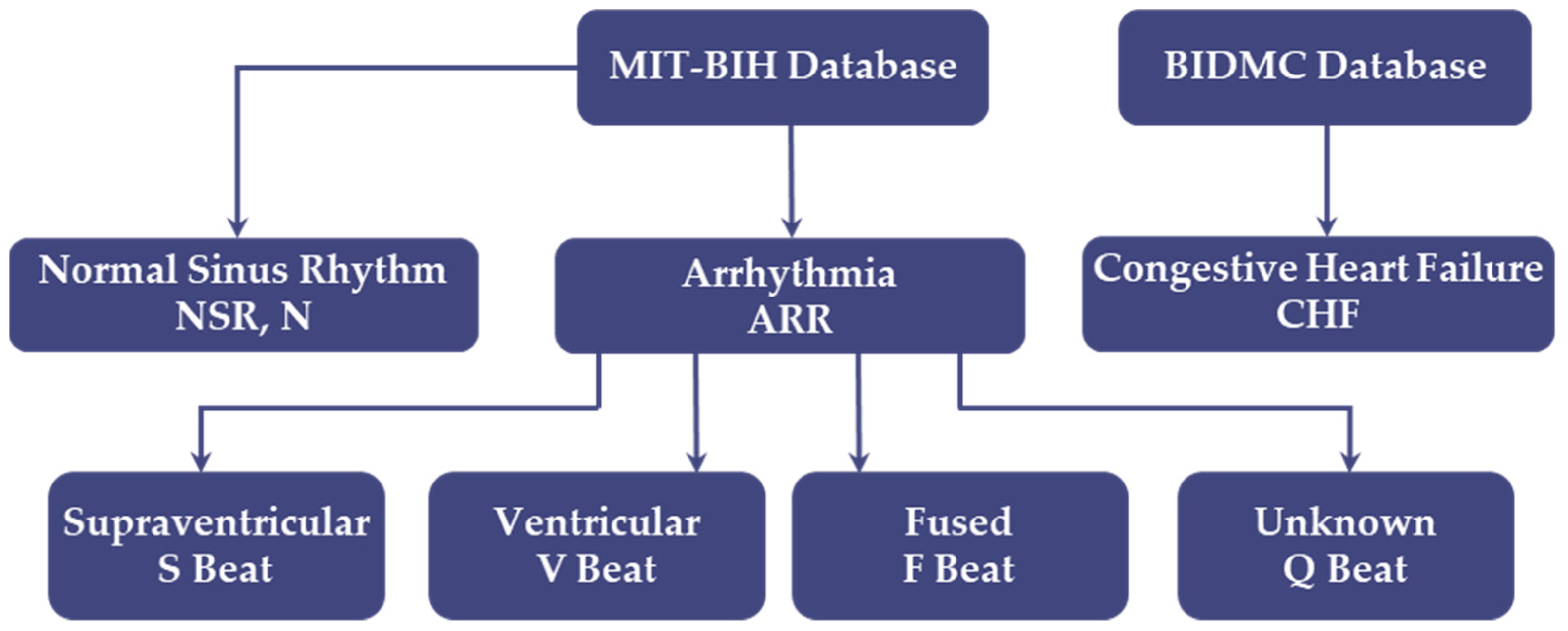
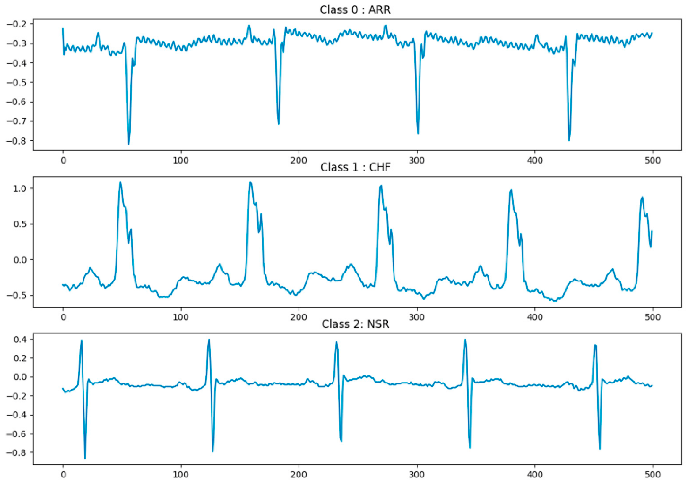
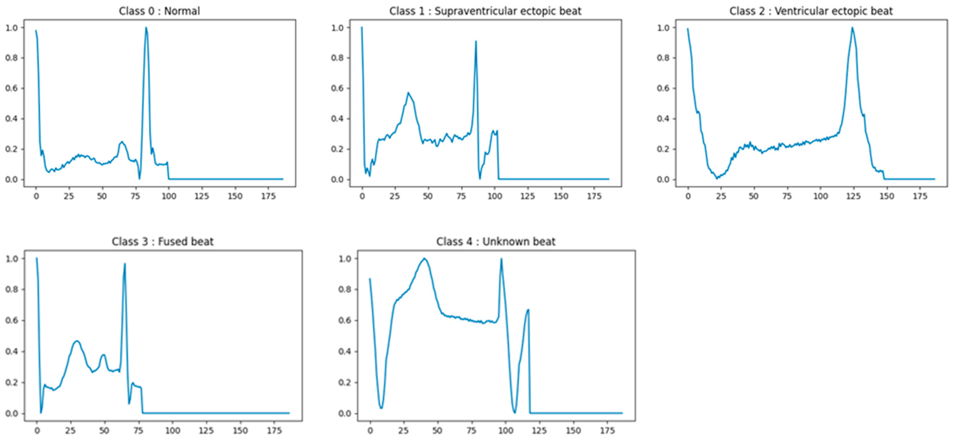
2.1. Dataset Preparation

Two key databases were used in this study to prepare the datasets for investigating heart rhythm:

MIT-BIH Arrhythmia Database: This collection focuses on electrocardiogram (ECG) recordings. It is known for having various arrhythmia types, making it ideal for developing and testing algorithms that detect and classify these irregular heartbeats [22].

BIDMC Congestive Heart Failure Database: This database from Harvard Medical School stores a wider range of medical data from patients with heart failure [23]. It includes ECGs alongside clinical notes, imaging scans, and other physiological signals. Figure 1 shows the structure of the databases, with corresponding subcategories, which were used to prepare the two datasets for training and evaluating the proposed model.

Two different datasets from these databases were prepared using different numbers of classes. In one dataset, we only used the MIT-BIH database with five classes (the normal sinus rhythm (NSR or N) class, supraventricular ectopic beat (S), ventricular ectopic beat (V), fused beat (F), and unknown beats (Q)), as shown in Figure 1. Four of these classes, S, V, F, and Q, represent various types of arrhythmias, each with irregularities in the ECG recording. The fifth, NSR or N, represents the normal beat, the baseline against which the other classes were judged.

The other dataset had three classes and was prepared by using normal and abnormal rhythms (normal sinus rhythm (NSR) and arrhythmia (ARR) classes) from the MIT-BIH database and the congestive heart failure (CHF) class from the BIDMC database.

For the three-class dataset, based on studies from the literature [19], we started with 162 recordings from three groups: arrhythmia (ARR), normal sinus rhythm (NSR), and congestive heart failure (CHF). The breakdown was 96 recordings for ARR, 30 for CHF, and 36 for NSR. We randomly selected 30 recordings from each class, resulting in a total of 90 recordings. Each recording initially had a massive sample with 65,536 features. We segmented this sample into smaller, non-overlapping intervals of 500 features each. This segmentation resulted in 131 samples for each original recording. Consequently, each class (ARR, NSR, CHF) had 3930 individual samples. In total, we had 11,790 samples, each of length 500, extracted from the 90 recordings. For the five-class dataset, which was collected only from the MIT-BIH database, we arranged samples of length 187, the same as what is presented in the literature. In total, the 5-class dataset had 10,000 samples equally distributed among the 5 classes.

Figure 2 and Figure 3 show examples of the segmented samples from the three-class and five-class ECG datasets of length 500 and 187, respectively.

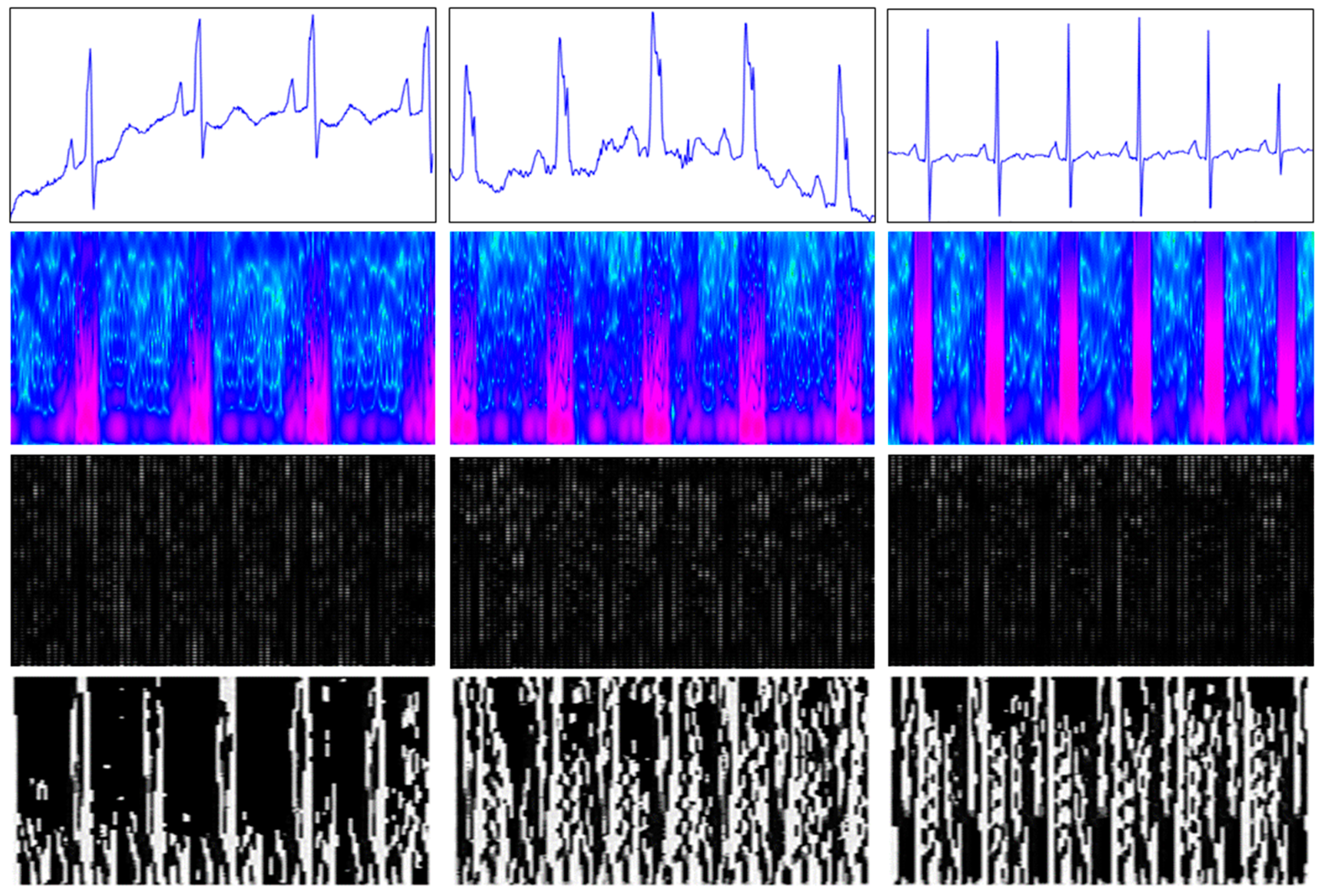
2.2. Generated Images

2.2.1. Spectrogram Image

Thinking of a heartbeat as an audio signal, a spectrogram helps us see the different pitches (frequencies) present in that signal over time. It does this by converting the ECG signal, originally existing in the time domain (showing changes over time), into the frequency domain (showing the mix of different frequencies). A technique called short-time Fourier transform (STFT) is used for this conversion [24]. STFT essentially breaks down the signal into smaller intervals and analyzes the frequencies present in each interval. By putting these frequency analyses together over time, we obtain a spectrogram. In a spectrogram, the x-axis and y-axis represent the time and frequency domains, respectively. This allows us to see how the frequencies within the signal change over time, revealing the different rhythmic components present in the heartbeat. The color intensity represents the strength of each frequency. Brighter colors indicate stronger frequencies at that time.

2.2.2. Local Binary Pattern (LBP) Image

Local binary pattern (LBP) is a popular method used to describe the textural features of images [25,26,27]. Introduced in 1996 [28] and later extended and popularized in 2002 [29], it essentially captures how pixels relate to their neighbors.

Consider a single pixel in an image. The LBP compares the intensity (brightness) of this pixel to its surrounding pixels. If a neighbor is brighter or equal in brightness, it is marked as 1; otherwise, it is marked as 0. These 1s and 0s are then combined in a specific order (like a code) to create a unique pattern for that central pixel. This pattern reflects the local texture around it.

By applying this process to all pixels, we obtain a new image where each pixel holds a code representing its local texture. Additionally, a histogram can be created to show how often each unique pattern appears in the image, revealing the overall texture distribution. Figure 4 visually demonstrates how the LBP code is calculated for a single pixel.

2.2.3. Histogram of Oriented Gradients (HOG) Image

Another helpful technique for analyzing images such as spectrograms is the histogram of oriented gradients (HOG) [30,31,32]. Introduced in 2005 [33], the HOG captures the overall shape and form within an image by looking at the direction and intensity of changes (gradients) in small image regions. As the spectrogram represents frequencies at different time intervals, the HOG helps us understand the shapes formed by these frequencies. It does this by dividing the spectrogram into small grids and analyzing the direction of the gradients (steepness) within each grid. By looking at the distribution of these gradient directions, the HOG builds a kind of fingerprint for the local shapes in the spectrogram.

Figure 5 (top row) showcases the ECG signals and respective spectrogram images (second row) for various ECG signals to visually analyze their frequency content. The third row of Figure 5 shows examples of HOG images derived from their respective spectrograms. These HOG images highlight the distinct shapes present in the frequency patterns of the ECG signals. The bottom row of Figure 5 showcases examples of LBP images derived from their respective spectrograms, highlighting their textural variations.

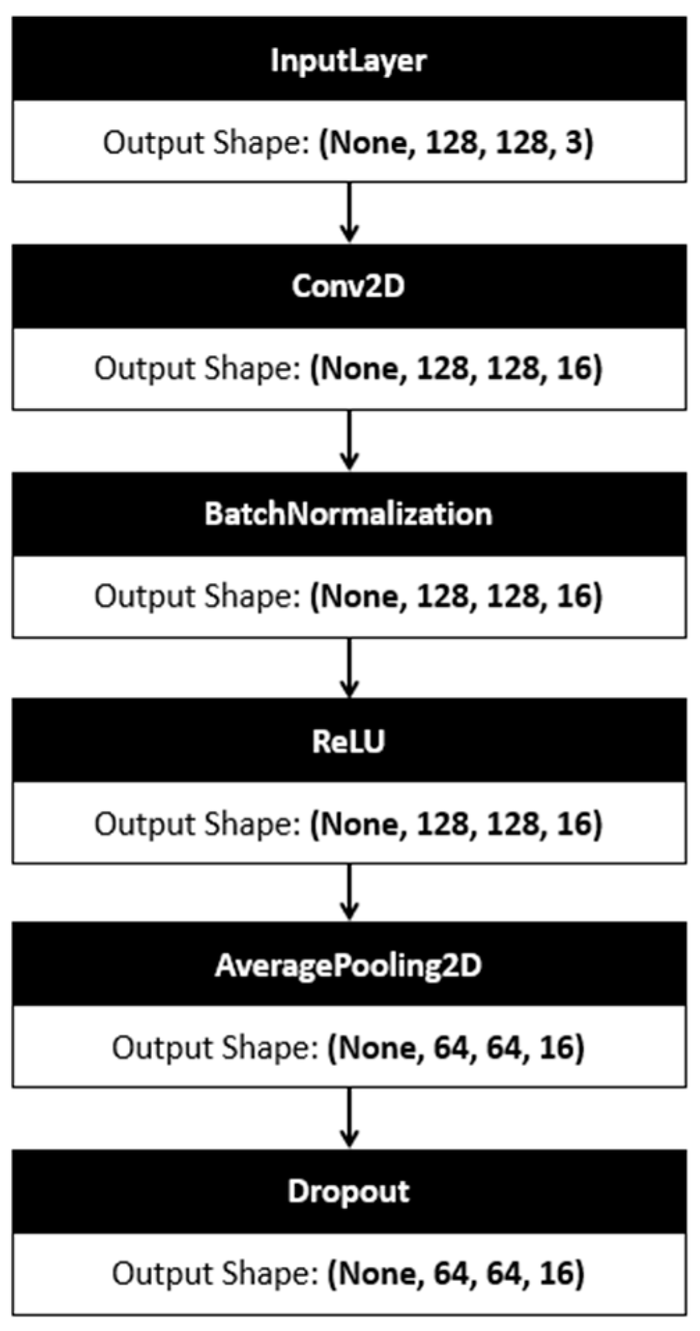
2.3. Deep Learning Algorithms

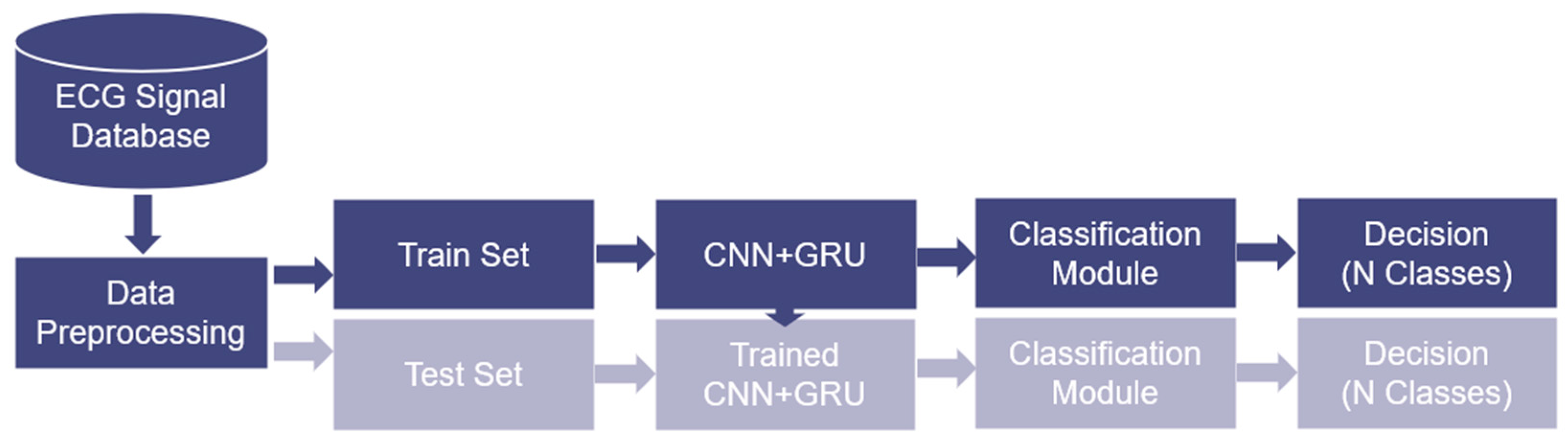
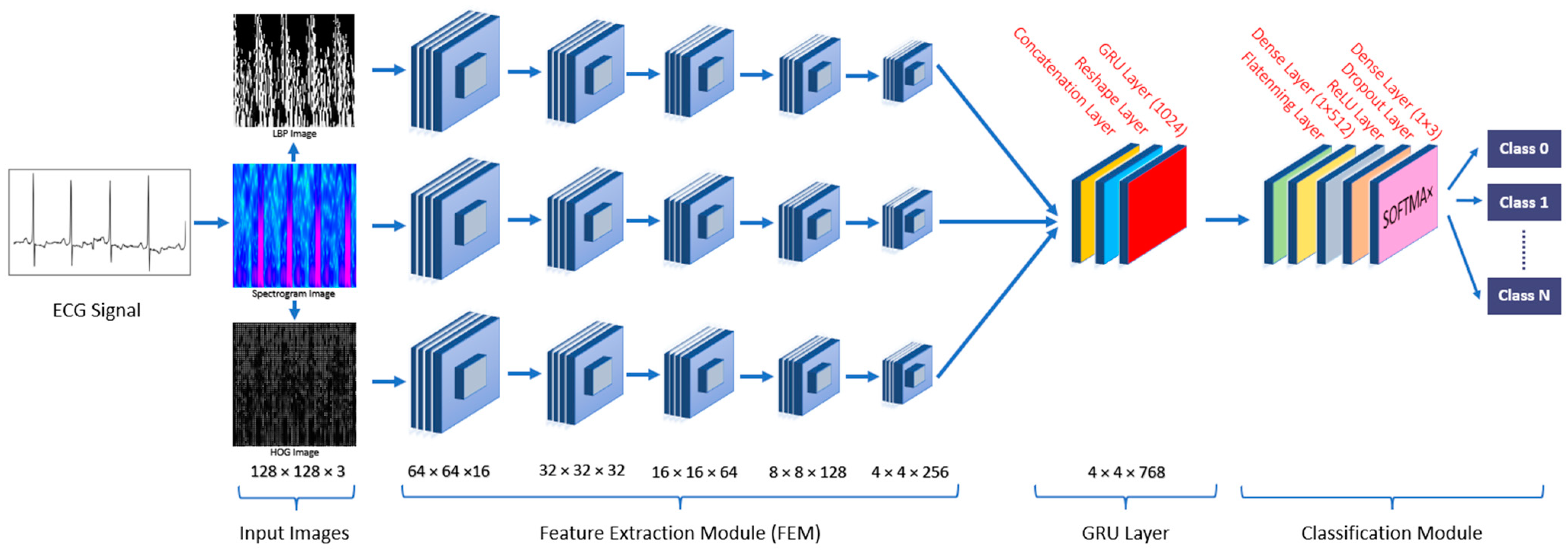
Deep learning has had a transformative impact on artificial intelligence (AI) and machine learning (ML). It lets us build powerful models that can learn subtle patterns hidden within massive datasets. At its core, deep learning uses special networks called deep neural networks with many layers stacked on top of each other. Imagine each layer as a filter that refines the information. As data travel through these layers, the network learns increasingly complex features. A big advantage of deep learning is that it can automatically discover these features directly from raw data, like images, sounds, or text. This saves us the time and effort of figuring them out manually, especially for complex data with higher dimensions.

Convolutional neural networks (CNNs), a class of deep neural networks designed specifically for processing images, have achieved remarkable success in applications such as object detection, image segmentation, and classification [34,35,36,37,38]. Recurrent neural networks (RNNs) are another type of deep neural network particularly suited for processing sequential data, such as time-series prediction and natural language processing (NLP). However, traditional RNNs can struggle with the vanishing gradient problem, making it difficult to learn long-term dependencies in data. Long short-term memory (LSTM) networks [39] and gated recurrent units (GRUs) [40] are variations of RNNs specifically designed to address this challenge. LSTMs and GRUs can remember information from earlier parts of a sequence and use it to understand later parts, effectively capturing long-range dependencies.

3. Methodology

There are several benefits to using spectrogram images in deep learning (DL) image classification tasks, especially when dealing with time-series data such as electrocardiogram (ECG) signals. Spectrograms convert ECG signals into a visual representation, essentially turning a time-series problem into an image classification problem. This allows us to leverage the power and well-established techniques of convolutional neural networks (CNNs), which have been highly successful in image recognition. CNNs can automatically learn the relevant features from the spectrogram image itself. This eliminates the need for manual feature engineering, which can be a complex and time-consuming process for data. Also, since spectrograms are already visual representations, they often require less preprocessing compared to raw data. This can save time and resources during the model development process. Moreover, unlike traditional images, spectrograms are often less affected by factors like background noise or slight variations in size. This can lead to more robust models. Overall, spectrograms offer a powerful approach for applying deep learning techniques to classification tasks. They can lead to more accurate and efficient models by leveraging the strengths of CNNs and reducing the need for manual feature engineering.

This work introduces a new deep learning spectrogram-based model for the classification of electrocardiogram (ECG) signals using feature fusion from the output of 3 CNN channels. As shown in the flowchart in Figure 6, at the data preprocessing stage, the proposed methodology converts the ECG time-series signal into a spectrogram image using a short-time Fourier transform (STFT). The spectrogram image is resized to 128 × 128 pixels and then used to generate another two images using HOG and LBP algorithms. The HOG and LBPs are often superior for feature extraction due to their efficiency and robustness. The HOG is excellent at detecting edges and shapes, making it effective for tasks like object detection while being robust to lighting variations. LBP excels in capturing local textures and is computationally efficient, making it ideal for texture classification. Both methods are resilient to changes in illumination, rotation, and scale, making them suitable for real-world applications where other descriptors may struggle with these variations. A 3 × 3 window size is used in both algorithms to generate the corresponding HOG and LBP images. Eight neighboring pixels in the LBP calculation and nine angle ranges in the HOG calculation were assigned as parameter values. Sample spectrogram images from the database and their corresponding LBP and HOG images are shown in Figure 5. After the preprocessing stage, the dataset is split into training and testing sets. For the training stage, the three images generated are used as inputs to a 2D convolutional neural network (CNN) model, which is a type of deep learning algorithm that is particularly effective for image classification tasks. To further enhance performance, a gated recurrent unit (GRU) model is added after the CNN model. A GRU is a type of recurrent neural network (RNN) that allows for the modeling of sequential data, making it ideal for analyzing time-series data such as ECG signals. After the classification model, the decision will be made to classify the input signal into one of the N classes (N = 3 or 5 classes) based on the dataset used.

This study developed a 3-channel CNN + GRU architecture with three input images. The architecture is designed such that each channel handles one of the three images: one for the RGB spectrogram image, another for the LBP image, and the last for the HOG image. In the proposed approach, each of the three input images is fed through its corresponding feature extraction module (FEM) in parallel. The FEM consists of 5 feature extraction (FE) blocks (see Figure 7).

Each FE block inside the FEM consists of five layers, namely the convolution layer, with a 3 × 3 filter size (which has filter outputs of sizes 16, 32, 64, 128, and 256 in each of the five FE blocks, respectively); the batch normalization layer; the ReLU activation layer; the average pooling layer, with a 2 × 2 pool size; and the dropout layer, with a ratio of 0.25, except for the last FE block, where the ratio is 0.5. The three outputs of the FEM obtained from the corresponding channels are fused into a single feature vector at the concatenation layer of the GRU module. The GRU module also consists of a reshape layer of size 16 × 768 and a GRU layer of 1024 units. For performance optimization, an average pooling layer and ReLU activation layer were favored over a max pooling layer and Leaky ReLU activation layer. The comparison results shown in Section 4 support this decision.

Finally, the classification module receives the output vector of the GRU module to process and classify it into one of the three classes. The classification module consists of a flattening layer, a dense layer of 512 neurons, a ReLU layer, a dropout layer, and a dense layer of 3 neurons (representing the three classes). The final decision is obtained at the dense layer using the SoftMax activation function. A block diagram of the proposed 3-channel fusion-based CNN + GRU architecture is shown in Figure 8.

4. Results and Discussion

As mentioned earlier, the two datasets used in the conducted experiments were prepared from the MIT-BIH and BIDMC databases. Details of the setup of the conducted experiments for the datasets are shown in

Table 1. Details of the two datasets used in the training and evaluation of the proposed model.

Datasets	No. of Classes	No. of Samples	Train	Test	Sample Length	Sample in Sec	Classes
MIT-BIH	5 classes	10,000	8000	2000	187	1.46	N, S, V, F, Q
MIT-BIH + BIDMC	3 classes	11,790	9432	2358	500	3.90	ARR, SNR, CHF

below. The MIT-BIH dataset contains 10,000 samples equally distributed among five classes. Each sample has a vector of length 187. The second dataset, MIT-BIH + BIDMC, has 11,790 samples, which are also equally distributed among three classes. These samples have a vector of length 500. Eighty percent of each dataset (8000 and 9432 samples, respectively) are used for training, and the remaining twenty percent (2000 and 2358 samples, respectively) are used for testing.

For the evaluation of the model, we used confusion matrices to calculate various performance metrics for our models. These confusion matrices contain information about how well the models classified different types of samples. For each class, we calculated the positive samples that the model correctly identified (true positives—TPs), the negative samples that the model correctly identified (true negatives—TNs), the negative samples that the model incorrectly classified as positive (false positives—FPs), and the positive samples that the model incorrectly classified as negative (false negatives—FNs). Using these values, we then calculated the overall performance metrics for the model:

Accuracy (Equation (1)): this represents the overall proportion of correctly classified samples.

Precision (Equation (2)): this measures how good the model is at identifying true positives without mistakenly including false positives.

Recall (Equation (3)): this measures how good the model is at identifying all true positives and avoiding false negatives.

F1-Score (Equation (4)): this is a harmonic mean that combines both precision and recall into a single metric.

By calculating these metrics, we can gain a comprehensive understanding of the model’s strengths and weaknesses in classifying different types of samples [41].

$$Accuracy={\displaystyle \frac{TP+TN}{TP+TN+FP+FN}}$$

(1)

$$Precision={\displaystyle \frac{TP}{TP+FP}}$$

(2)

$$Recall={\displaystyle \frac{TP }{TP+FN}}$$

(3)

$$F1-Score={\displaystyle \frac{2\times Precision\times Recall}{Precision+Recall}}$$

(4)

All the models were programmed and experiments were conducted for this research using Python 3.10.14 in the user-friendly cloud environment Kaggle, a subsidiary of Google. TensorFlow, a popular library for machine learning, and Keras, a high-level interface for TensorFlow, were used to build and evaluate the CNN + GRU models.

4.1. Ablation Study

To strengthen the validation of our proposed three-channel fusion-based CNN + GRU model, we conducted an ablation study focusing on the impact of different activation functions and pooling layers. Specifically, we compared the performance of the model using two activation functions, ReLU and Leaky ReLU, along with two types of pooling layers, average pooling and max pooling.

Table 2. Performance comparison of CNN + GRU using different pooling layers and activation functions on two datasets.

	3-Class Dataset (MIT-BIH + BIDMC)		5-Class Dataset (MIT-BIH)
Parameters	Accuracy	Loss	Accuracy	Loss
ReLU + Average Pooling	99.796	0.0106	99.780	0.0246
ReLU + Max Pooling	98.922	0.0359	96.969	0.1098
Leaky ReLU + Average Pooling	99.270	0.0214	99.760	0.0285
Leaky ReLU + Max Pooling	98.905	0.0364	90.589	0.3724

presents a performance comparison of a CNN + GRU model on two datasets: a three-class dataset (MIT-BIH + BIDMC) and a five-class dataset (MIT-BIH). The metrics used are accuracy and loss, with variations depending on the activation functions (ReLU and Leaky ReLU) and pooling layers (average pooling and max pooling). A comparative analysis of average pooling and max pooling within the proposed model demonstrated that average pooling consistently outperformed max pooling. Furthermore, the ReLU activation function exhibited marginally better performance than Leaky ReLU. As summarized in Table 2, ReLU with average pooling consistently performs the best across both datasets. Max pooling generally results in lower accuracy and higher loss, particularly for the five-class dataset. Leaky ReLU + max pooling shows the worst performance, especially on the five-class dataset, with accuracy dropping sharply. The combination of ReLU + average pooling seems to be optimal for this CNN + GRU model at each block of both the FEM and GRU networks across both datasets.

To further highlight the advantages of our proposed three-channel fusion-based CNN + GRU model, we conducted another ablation study to analyze the impact of each input channel (spectrogram, LBP, and HOG images) on the overall model performance.

Table 3. Comparison between the proposed 3-channel fusion-based CNN + GRU model and the corresponding 1-channel versions for the 3-class dataset (MIT-BIH + BIDMC).

	3-Channel Model	1-Channel Model
		Spectrogram	LBP	HOG
Training time (min)	3.48	1.47	1.46	1.74
Prediction time (sec/image)	0.0027	0.0010	0.0010	0.0010
Loss rate	0.0189	0.29	0.029	0.031
Accuracy rate	99.75	98.69	98.53	98.51

illustrates the comparison between the proposed three-channel fusion-based CNN + GRU model and the one-channel CNN + GRU models for the three-class dataset (MIT-BIH + BIDMC), where the latter utilizes only one of the three input images. While the training and average prediction times for the fusion-based model are longer than those for the one-channel CNN + GRU models, this increased duration should not pose a significant concern, as the training is a one-time offline process. Conversely, the three-channel fusion-based model demonstrates superior performance, achieving improved loss rates and accuracy.

Overall, this ablation study reinforces the effectiveness of our proposed model by emphasizing the importance of careful architectural design in achieving optimal results for ECG classification tasks.

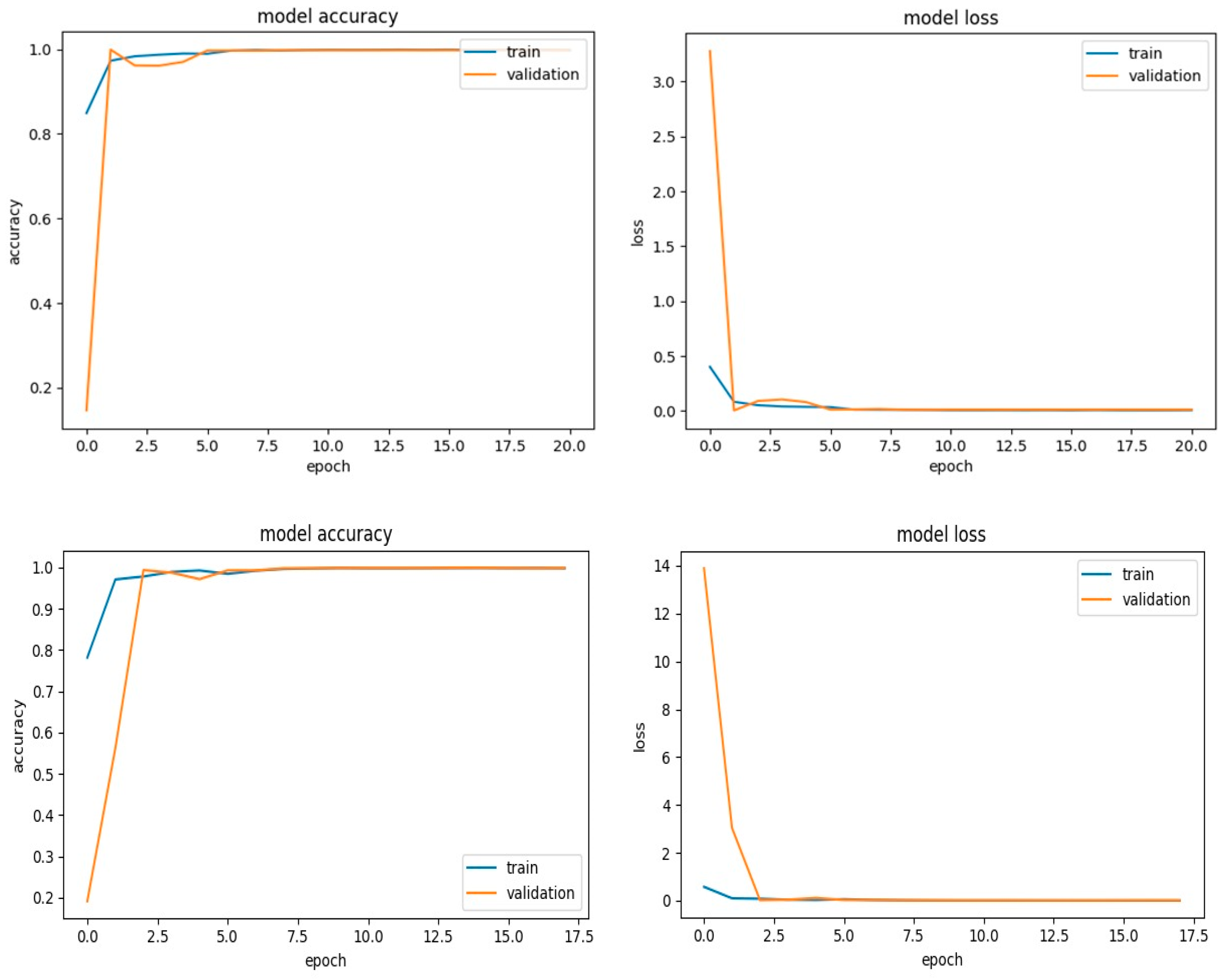
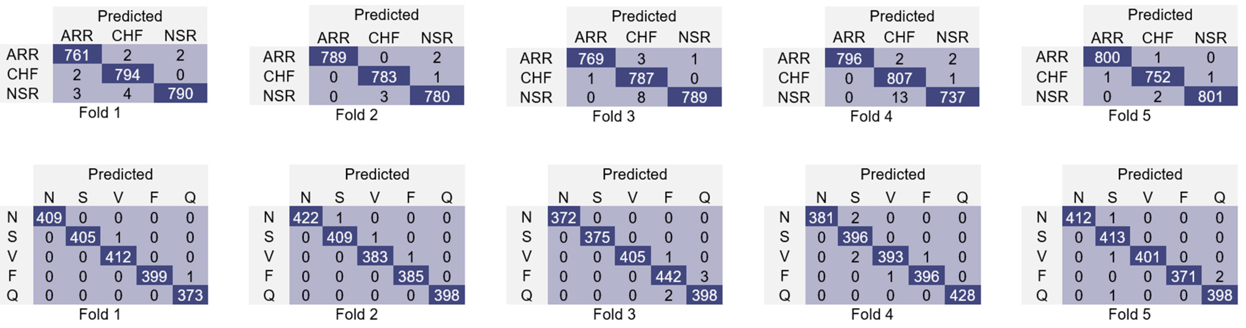
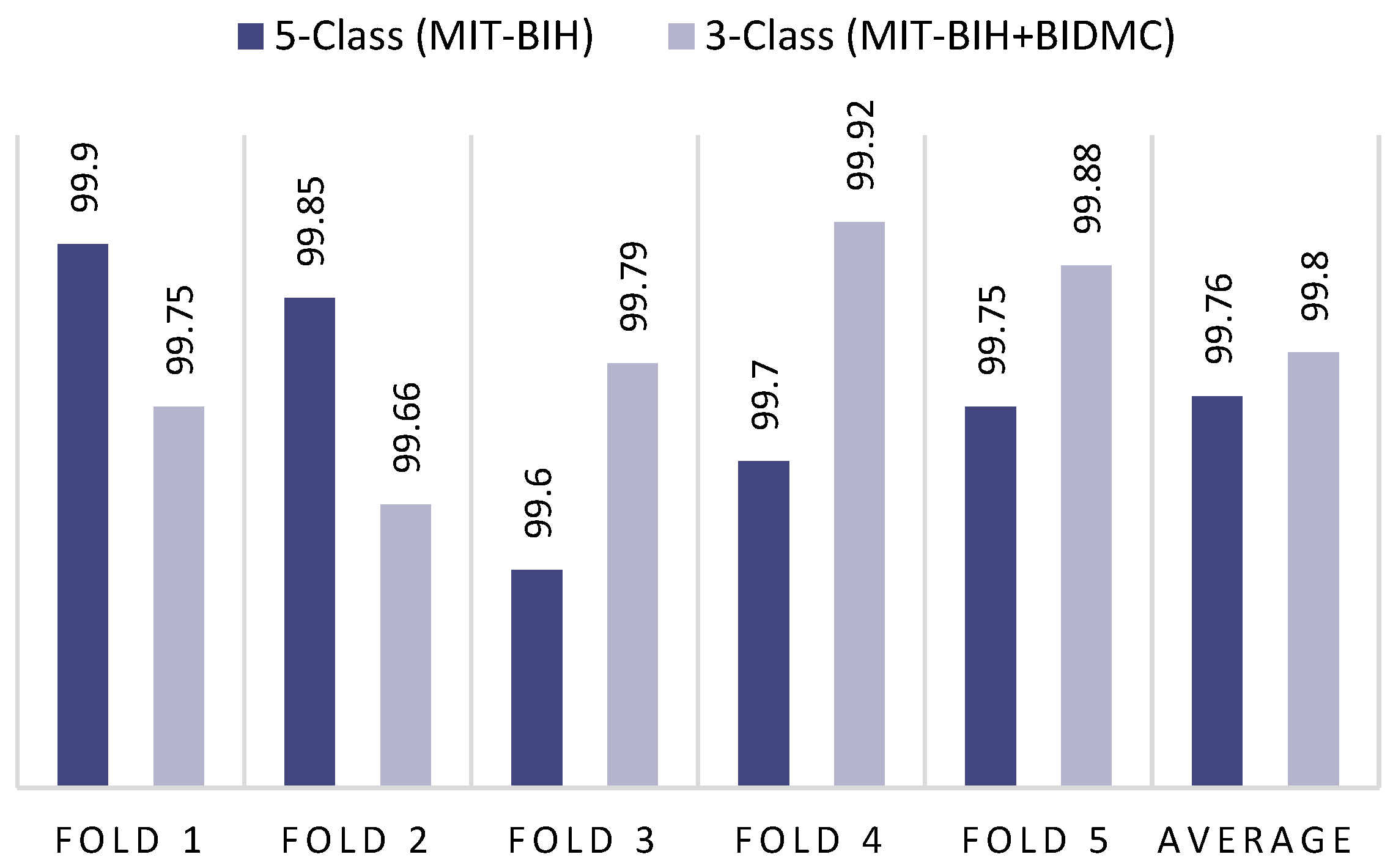
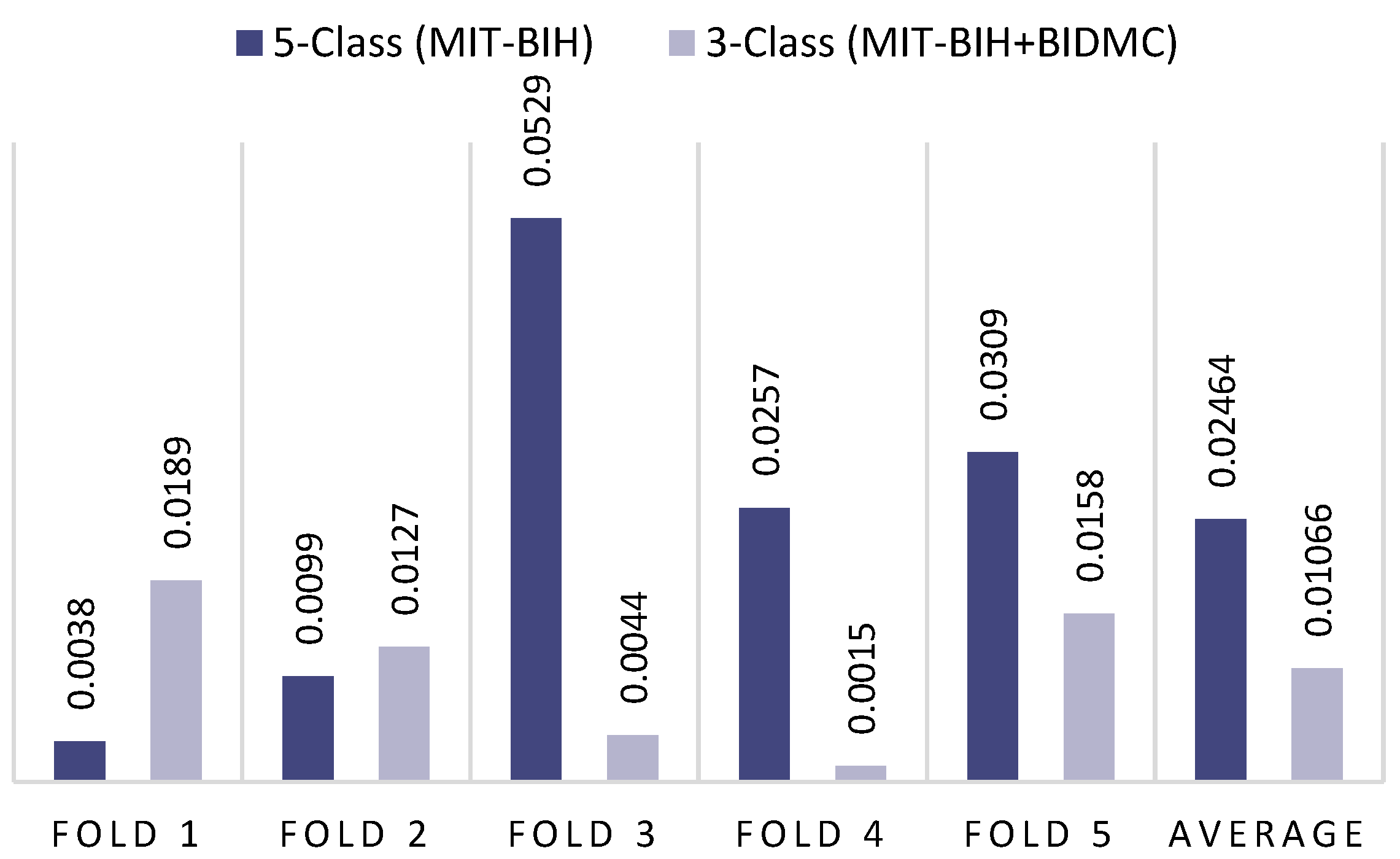
4.2. Simulation Results

To train the models effectively, we used a technique called Adam to optimize their performance and categorical cross-entropy to measure errors. Additionally, five-fold cross-validation was employed to assess the models’ accuracy by splitting the data into five equal subsets, ensuring no overlap. During training, we used three of these subsets for training, one for fine-tuning the model (validation), and the remaining one for final testing. This ensures all data points contribute to the training process at least once, while a dedicated subset is used for the final evaluation.

We trained the two CNN + GRU models for both datasets for 30 epochs (iterations). We fed the data in batches with a batch size of 32. Figure 9 illustrates an example of how the accuracy of the two models improved, and their errors (loss) decreased during training for the last fold (fold 5). It is important to note that for each of the five folds, we built and trained the two models from scratch. This means we separately obtained the five confusion matrices that summarize the performance of the two models on each data split. Figure 10 displays these confusion matrices for both models, applied to the three-class and five-class datasets, one for each fold of the evaluation process.

The confusion matrices from Figure 10 are used to calculate various performance metrics for our models. The performance of the proposed CNN + GRU model is evaluated using five-fold cross-validation on both a three-class dataset (MIT-BIH + BIDMC) and a five-class dataset (MIT-BIH), and the results in

Table 4. Five-fold cross-validation performance scores for the proposed CNN + GRU model.

	3-Class Dataset (MIT-BIH + BIDMC)				5-Class Dataset (MIT-BIH)
	Precision	Recall	F1-Score	Accuracy	Precision	Recall	F1-Score	Accuracy
1st Fold	99.75	99.75	99.75	99.75	99.90	99.90	99.90	99.90
2nd Fold	99.66	99.66	99.66	99.66	99.85	99.85	99.85	99.85
3rd Fold	99.79	99.79	99.79	99.79	99.60	99.60	99.60	99.60
4th Fold	99.92	99.92	99.92	99.92	99.70	99.70	99.70	99.70
5th Fold	99.87	99.87	99.87	99.88	99.75	99.75	99.75	99.75
Average	99.80	99.80	99.80	99.80	99.76	99.76	99.76	99.76

demonstrate consistently high metrics across the board. For the three-class dataset, the model achieves near-perfect precision, recall, F1-score, and accuracy, with values ranging from 99.66% to 99.92% across all folds, culminating in an average score of 99.80% for each metric. This indicates that the model is highly reliable, with minimal variance between folds, and consistently performs well in classifying the three categories. On the five-class dataset, the model maintains an impressive level of performance, with precision, recall, F1-score, and accuracy ranging between 99.60% and 99.90%, resulting in an average score of 99.76% across all metrics. Although slightly lower than the three-class dataset, this performance is still exceptional, suggesting that the model is capable of handling the increased complexity of classifying five different classes. The consistency in performance across all folds for both datasets underscores the robustness of the CNN + GRU model, which generalizes well to different data subsets, making it a reliable choice for both classification tasks. However, the slight decrease in performance for the five-class dataset may be attributed to the increased challenge of distinguishing between more classes, but the drop is minimal, highlighting the model’s strong overall effectiveness.

To assess the performance of the CNN + GRU algorithms, we compared their accuracies across five folds for both test sets and calculated the average values. The results are depicted in Figure 11. This figure contrasts the performance on the three-class (MIT-BIH + BIDMC) and five-class (MIT-BIH) datasets. While the three-class dataset achieved slightly higher accuracy, the CNN + GRU model exhibited almost double the loss value for the five-class dataset. These trends are expected given the increased number of classes in the latter. Figure 12 illustrates the corresponding loss values for both models.

Table 5. Comparison of the proposed model against other models from the literature.

Ref.	Year	Datasets	Algorithm	Train/TestRatio	No. of Classes	Precision	Recall	F1-Score	Accuracy
[13]	2021	MIT-BIH AF	CNN + LSTM	90/10	4	-	97.87	-	-
[14]	2022	St. Petersburg	DW-CMT + TCP+SVM	90/10	4	97.80	97.80	97.80	97.80
[42]	2022	MIT-BIH AF	CNN + Transformers	90/10	4	95.38	92.51	93.88	99.49
[10]	2017	MIT-BIH	9 layers CNN	90/10	5	97.86	96.71	97.28	94.03
[12]	2021	MIT-BIH	CNN + GA	80/20	5	95.80	99.70	89.70	98.00
[14]	2022	MIT-BIH	DW-CMT + TCP + kNN	90/10	5	95.18	98.51	96.69	96.60
[15]	2022	MIT-BIH	CBAM-ResNet	80/20	5	99.13	97.50	98.29	99.23
[19]	2024	MIT-BIH	FT + CNN-LSTM	80/20	5	97.30	97.40	97.30	97.40
[36]	2022	MIT-BIH	CNN + RF	80/20	5	76.00	78.00	74.00	96.00
[37]	2023	MIT-BIH	CNN	90/10	5	92.86	92.41	92.63	98.63
[38]	2021	MIT-BIH	CWT + CNN	50/50	5	70.75	67.47	68.76	98.74
[43]	2018	MIT-BIH AF	SWT + DCNN	90/10	5	-	98.79	-	98.63
[44]	2022	MIT-BIH	ResNet + BiLSTM	80/20	5	92.23	91.23	91.69	99.20
[45]	2022	MIT-BIH	CNN + TTM	90/10	5	48.10	70.60	57.12	96.36
[46]	2022	MIT-BIH	SE-ResNet	90/10	5	93.87	93.78	93.82	99.61
[47]	2023	MIT-BIH	RPM + Gam-Resnet18	80/20	5	98.76	98.90	-	99.30
Ours	2024	MIT-BIH	3-Channel CNN + GRU	80/20	5	99.76	99.76	99.76	99.76
[48]	2022	MIT-BIH + BIDMC	LSTM	80/20	3	-	-	-	96.00
[49]	2021	MIT-BIH + BIDMC	CWT + AlexNet	-	3	97.70	97.80	97.70	97.8
[50]	2022	MIT-BIH + BIDMC	CWT + CNN + LSTM	90/10	3	98.00	98.00	97.30	98.90
[51]	2023	MIT-BIH + BIDMC	ResNet50	80/20	3	99.20	99.20	99.20	99.20
Ours	2024	MIT-BIH + BIDMC	3-Channel CNN + GRU	80/20	3	99.80	99.80	99.80	99.80

presents a comparison of various algorithms used for arrhythmia detection across different datasets and time periods, with metrics such as precision, recall, F1-score, and accuracy.

From the dataset perspective, these results demonstrate the effectiveness of different algorithms on various ECG datasets, such as MIT-BIH, MIT-BIH AF, and BIDMC. The MIT-BIH dataset can be considered a benchmark for ECG classification, with algorithms typically addressing a four- or five-class classification problem. Notably, the recent results demonstrate a clear progression in performance, with hybrid and deep learning models like ResNet, CNN + GRU, and ResNet + BiLSTM achieving superior results across all metrics. For instance, the proposed model, using a three-channel CNN + GRU on both the MIT-BIH and MIT-BIH + BIDMC datasets, achieves remarkable precision, recall, F1-score, and accuracy values, indicating near-perfect classification ability. This surpasses earlier models such as CNN + Transformers and ResNet + BiLSTM, which, while achieving high accuracies, did not achieve as consistently high values across all metrics.

Focusing on five-class classifications in the MIT-BIH dataset, earlier methods like using a CNN with genetic algorithms (CNN + GA) achieved a precision of 95.80% and an accuracy of 98.00% but had a notably lower F1-score of 89.70%, indicating weaker performance in balancing precision and recall. More recent algorithms, such as CBAM-ResNet, showed significant improvements, with a precision of 99.13%, an F1-score of 98.29%, and an accuracy of 99.23%. This highlights the advancements made in integrating attention mechanisms into models. The proposed three-channel CNN + GRU model outperforms all previous methods on the five-class MIT-BIH dataset, achieving a perfect balance with 99.76% across precision, recall, F1-score, and accuracy, showcasing its superior ability to classify arrhythmia types.

For the three-class datasets (MIT-BIH + BIDMC), methods like CWT + CNN + LSTM performed well, with a precision and recall of 98.00% and an accuracy of 98.90%. The ResNet50 achieved notable results, with precision, recall, F1-score, and accuracy consistently at 99.20%. However, the proposed three-channel CNN + GRU model stands out as the best performer, delivering 99.80% across all metrics. This demonstrates the model’s robustness in both three-class and five-class arrhythmia detection, achieving near-perfect results and surpassing previous state-of-the-art techniques.

While the proposed method appears to have potentially greater computational complexity compared to existing approaches, this complexity can be justified by the noticeable improvement in performance. With advances in modern hardware, such as more powerful processors (e.g., GPUs and TPUs) and specialized hardware for machine learning, the relative difference in computation time between the proposed method and less complex approaches may be reduced to mere milliseconds. This minimal difference in runtime, particularly on state-of-the-art hardware, becomes a negligible trade-off when considering the performance gains. Moreover, in many practical applications, small improvements in accuracy or reliability can have significant impacts, making the slight increase in computational complexity well worth the benefits, especially in high-throughput systems where precision matters.

5. Conclusions

This paper tackled ECG signal classification with a new deep learning approach. The raw time-series ECG signal is transformed into a visual representation called a spectrogram using STFT. This spectrogram shows how the frequencies within the signal change over time. To capture deeper insights from the spectrogram, two techniques are applied: HOG, which analyzes the direction and intensity of changes (gradients) within small regions of the spectrogram, and LBP, which focuses on how individual pixels in the spectrogram relate to their neighbors. This creates a code representing the local texture around each pixel, highlighting textural variations within the spectrogram. Three images are generated: the original spectrogram, along with the corresponding HOG and LBP images. These are then fed into a 2D convolutional neural network (CNN). A CNN is particularly adept at recognizing patterns within images. In this case, the CNN learns to identify specific patterns in the spectrograms, HOG, and LBP images that are indicative of different ECG classes. To further enhance the model’s accuracy, a gated recurrent unit (GRU) is added after the CNN. GRUs are a type of recurrent neural network (RNN) that excels at handling sequential data like ECG signals. The GRU takes the combined outputs from the three-channel CNN and analyzes them over time, potentially capturing even more subtle features that contribute to classification. The model was rigorously tested on two datasets containing data representing three and five different classes. The results were impressive, demonstrating that the combination of spectrogram representation, feature fusion, and the CNN-GRU model outperforms existing algorithms, as shown in the last table.

This suggests that the proposed method has significant potential for accurate ECG classification, which is crucial for diagnosing and treating various cardiovascular diseases. By effectively identifying patterns in ECG signals, this approach could become a valuable tool in cardiology. This also reflects the growing sophistication of models and their ability to handle ECG data with greater accuracy and reliability, indicating that newer methods are leveraging both the richness of these datasets and advancements in deep learning techniques to push the boundaries of performance.

References

1. Dubatovka, A. Interpretable and robust Machine Learning Models for Time-Series Analysis in Cardiology. Doctoral Dissertation, ETH Zurich, Zurich, Switzerland, 2024. [Google Scholar] [CrossRef]
2. Haseena, H.H.; Joseph, P.K.; Mathew, A.T. Classification of arrhythmia using hybrid networks. J. Med. Syst. 2011, 35, 1617–1630. [Google Scholar] [CrossRef] [PubMed]
3. Sannino, G.; De Pietro, G. A deep learning approach for ECG-based heartbeat classification for arrhythmia detection. Future Gener. Comput. Syst. 2018, 86, 446–455. [Google Scholar] [CrossRef]
4. Çınar, A.; Tuncer, S.A. Classification of normal sinus rhythm, abnormal arrhythmia and congestive heart failure ECG signals using LSTM and hybrid CNN-SVM deep neural networks. Comput. Methods Biomech. Biomed. Eng. 2021, 24, 203–214. [Google Scholar] [CrossRef] [PubMed]
5. Eleyan, A.; AlBoghbaish, E.; AlShatti, A.; AlSultan, A.; AlDarbi, D. RHYTHMI: A deep learning-based mobile ECG device for heart disease prediction. Appl. Syst. Innov. 2024, 7, 77. [Google Scholar] [CrossRef]
6. Qammar, N.W.; Vainoras, A.; Navickas, Z.; Jaruševičius, G.; Ragulskis, M. Early Diagnosis of Atrial Fibrillation Episodes: Comparative Analysis of Different Matrix Architectures. Appl. Sci. 2024, 14, 6191. [Google Scholar] [CrossRef]
7. Deng, J.; Ma, J.; Yang, J.; Liu, S.; Chen, H.; Wang, X.; Zhang, X. An Energy-Efficient ECG Processor Based on HDWT and a Hybrid Classifier for Arrhythmia Detection. Appl. Sci. 2024, 14, 342. [Google Scholar] [CrossRef]
8. Kiranyaz, S.; Ince, T.; Gabbouj, M. Real-time patient-specific ECG classification by 1-D convolutional neural networks. IEEE Trans. Biomed. Eng. 2016, 63, 664–675. [Google Scholar] [CrossRef]
9. Jeong, Y.; Lee, J.; Shin, M. Enhancing Inter-Patient Performance for Arrhythmia Classification with Adversarial Learning Using Beat-Score Maps. Appl. Sci. 2024, 14, 7227. [Google Scholar] [CrossRef]
10. Acharya, U.R.; Oh, S.L.; Hagiwara, Y.; Tan, J.H.; Adam, M.; Gertych, A.; San Tan, R. A deep convolutional neural network model to classify heartbeats. Comput. Biol. Med. 2017, 89, 389–396. [Google Scholar] [CrossRef]
11. Hannun, A.Y.; Rajpurkar, P.; Haghpanahi, M.; Tison, G.H.; Bourn, C.; Turakhia, M.P.; Ng, A.Y. Cardiologist-level arrhythmia detection and classification in ambulatory electrocardiograms using a deep neural network. Nat. Med. 2019, 25, 65–69. [Google Scholar] [CrossRef]
12. Hammad, M.; Iliyasu, A.M.; Subasi, A.; Ho, E.S.L.; El-Latif, A.A.A. A multitier deep learning model for arrhythmia detection. IEEE Trans. Instrum. Meas. 2021, 70, 2502809. [Google Scholar] [CrossRef]
13. Petmezas, G.; Haris, K.; Stefanopoulos, L.; Kilintzis, V.; Tzavelis, A.; Rogers, J.A.; Katsaggelos, A.K.; Maglaveras, N. Automated atrial fibrillation detection using a hybrid CNN-LSTM network on imbalanced ECG datasets. Biomed. Signal Process. Control 2021, 63, 102194. [Google Scholar] [CrossRef]
14. Tuncer, T.; Dogan, S.; Plawiak, P.; Subasi, A. A novel discrete wavelet-concatenated mesh tree and ternary chess pattern-based ECG signal recognition method. Biomed. Signal Process. Control 2022, 72, 103331. [Google Scholar] [CrossRef]
15. Ma, K.; Zhan, C.A.; Yang, F. Multi-classification of arrhythmias using ResNet with CBAM on CWGAN-GP augmented ECG Gramian Angular Summation Field. Biomed. Signal Process. Control 2022, 77, 103684. [Google Scholar] [CrossRef]
16. Merbouti, M.A.; Cherifi, D. Machine learning based electrocardiogram peaks analyzer for Wolff-Parkinson-White syndrome. Biomed. Signal Process. Control 2023, 86, 105302. [Google Scholar] [CrossRef]
17. Park, J.; Lee, K.; Park, N.; You, S.C.; Ko, J. Self-attention LSTM-FCN model for arrhythmia classification and uncertainty assessment. Artif. Intell. Med. 2023, 142, 102570. [Google Scholar] [CrossRef]
18. Yang, X.; Zhang, A.; Zhao, C.; Yang, H.; Dou, M. Categorization of ECG signals based on the dense recurrent network. Signal Image Video Process. 2024, 18, 3373–3381. [Google Scholar] [CrossRef]
19. Eleyan, A.; Alboghbaish, E. Electrocardiogram signals classification using deep-learning-based incorporated convolutional neural network and long short-term memory framework. Computers 2024, 13, 55. [Google Scholar] [CrossRef]
20. Prusty, M.R.; Pandey, T.N.; Lekha, P.S.; Lellapalli, G.; Gupta, A. Scalar invariant transform-based deep learning framework for detecting heart failures using ECG signals. Sci. Rep. 2024, 14, 2633. [Google Scholar] [CrossRef]
21. Eleyan, A.; Alboghbaish, E.; Eleyan, G. Performance comparison between transform-based deep learning approaches for ECG signal classification. In Proceedings of the 11th International Conference on Electrical & Electronics Engineering (ICEEE24), Marmaris, Turkey, 22–24 April 2024. [Google Scholar]
22. Moody, G.B.; Mark, R.G. The impact of the MIT-BIH arrhythmia database. IEEE Eng. Med. Biol. Mag. 2001, 20, 45–50. [Google Scholar] [CrossRef]
23. Baim, D.S.; Colucci, W.S.; Monrad, E.S.; Smith, H.S.; Wright, R.F.; Lanoue, A.; Gauthier, D.F.; Ransil, B.J.; Grossman, W.; Braunwald, E. Survival of patients with severe congestive heart failure treated with oral milrinone. J. Am. Coll. Cardiol. 1986, 7, 661–670. [Google Scholar] [CrossRef] [PubMed]
24. Portnoff, M. Time-frequency representation of digital signals and systems based on short-time Fourier analysis. IEEE Trans. Acoust. Speech Signal Process 1980, 28, 55–69. [Google Scholar] [CrossRef]
25. Zhao, G.; Pietikainen, M. Dynamic texture recognition using local binary patterns with an application to facial expressions. IEEE Trans. Pattern Anal. Mach. Intell. 2007, 29, 915–928. [Google Scholar] [CrossRef]
26. Eleyan, A. Face recognition using ensemble statistical local descriptors. J. King Saud Univ.-Comput. Inf. Sci. 2023, 35, 9. [Google Scholar] [CrossRef]
27. Basar, S.; Ali, M.; Ochoa-Ruiz, G.; Waheed, A.; Rodriguez-Hernandez, G.; Zareei, M. A novel defocused image segmentation method based on PCNN and LBP. IEEE Access 2021, 9, 87219–87240. [Google Scholar] [CrossRef]
28. Ojala, T.; Pietikäinen, M.; Harwood, D. A comparative study of texture measures with classification based on featured distributions. Pattern Recognit. 1996, 29, 51–59. [Google Scholar] [CrossRef]
29. Ojala, T.; Pietikainen, M.; Maenpaa, T. Multiresolution grayscale and rotation invariant texture classification with local binary patterns. IEEE Trans. Pattern Anal. Mach. Intell. 2002, 24, 971–987. [Google Scholar] [CrossRef]
30. Eleyan, A. Statistical local descriptors for face recognition: A comprehensive study. Multimed. Tools Appl. 2023, 82, 32485–32504. [Google Scholar] [CrossRef]
31. Ji, P.; Feng, J.; Ma, F.; Wang, X.; Li, C. Fingertip detection algorithm based on maximum discrimination hog feature in complex background. IEEE Access 2023, 11, 3160–3173. [Google Scholar] [CrossRef]
32. Karakaya, F.; Altun, H.; Cavuslu, M.A. Implementation of HOG algorithm for real-time object recognition applications on FPGA based embedded system. In Proceedings of the 2009 IEEE 17th Signal Processing and Communications Applications Conference, Antalya, Turkey, 9–11 April 2009; pp. 508–511. [Google Scholar]
33. Dalal, N.; Triggs, B. Histograms of oriented gradients for human detection. In Proceedings of the 2005 IEEE Computer Society Conference on Computer Vision and Pattern Recognition (CVPR’05), San Diego, CA, USA, 20–25 June 2005; pp. 886–893. [Google Scholar]
34. Liu, S.; Wang, L.; Yue, W. An efficient medical image classification network based on multi-branch CNN, token grouping Transformer and mixer MLP. Appl. Soft Comput. 2024, 153, 111323. [Google Scholar] [CrossRef]
35. Bayram, F.; Eleyan, A. COVID-19 detection on chest radiographs using feature fusion-based deep learning. Signal Image Video Process. 2022, 16, 1455–1462. [Google Scholar] [CrossRef] [PubMed]
36. Zou, C.; Muller, A.; Wolfgang, U.; Ruckert, D.; Muller, P.; Becker, M.; Steger, A.; Martens, E. Heartbeat classification by random forest with a novel context feature: A segment label. IEEE J. Transl. Eng. Health Med. 2022, 10, 1900508. [Google Scholar] [CrossRef] [PubMed]
37. Khan, F.; Yu, X.; Yuan, Z.; Rehman, A.U. ECG classification using 1-D convolutional deep residual neural network. PLoS ONE 2023, 18, 4. [Google Scholar] [CrossRef] [PubMed]
38. Wang, T.; Lu, C.; Sun, Y.; Yang, M.; Liu, C.; Ou, C. Automatic ECG classification using continuous wavelet transform and convolutional neural network. Entropy 2021, 23, 119. [Google Scholar] [CrossRef]
39. Hochreiter, S.; Schmidhuber, J. Long short-term memory. Neural Comput. 1997, 9, 1735–1780. [Google Scholar] [CrossRef]
40. Chung, J.; Gulcehre, C.; Cho, K.; Bengio, Y. Empirical evaluation of gated recurrent neural networks on sequence modeling. arXiv 2024, arXiv:1412.3555. [Google Scholar]
41. Bolboacă, S.D.; Jäntschi, L. Predictivity Approach for Quantitative Structure-Property Models. Application for Blood-Brain Barrier Permeation of Diverse Drug-Like Compounds. Int. J. Mol. Sci. 2011, 12, 4348–4364. [Google Scholar] [CrossRef]
42. Hu, R.; Chen, J.; Zhou, L. A transformer-based deep neural network for arrhythmia detection using continuous ECG signals. Comput. Biol. Med. 2022, 144, 105325. [Google Scholar] [CrossRef]
43. Xia, Y.; Wulan, N.; Wang, K.; Zhang, H. Detecting atrial fibrillation by deep convolutional neural networks. Comput. Biol. Med. 2018, 93, 84–92. [Google Scholar] [CrossRef]
44. Kim, Y.K.; Lee, M.; Song, H.S.; Lee, S.-W. Automatic cardiac arrhythmia classification using residual network combined with long short-term memory. IEEE Trans. Instrum. Meas. 2022, 71, 4005817. [Google Scholar] [CrossRef]
45. Zubair, M.; Yoon, C. Cost-sensitive learning for anomaly detection in imbalanced ECG data using convolutional neural networks. Sensors 2022, 22, 4075. [Google Scholar] [CrossRef] [PubMed]
46. Li, X.; Zhang, F.; Sun, Z.; Li, D.; Kong, X.; Zhang, Y. Automatic heartbeat classification using S-shaped reconstruction and a squeeze-and-excitation residual network. Comput. Biol. Med. 2022, 140, 105108. [Google Scholar] [CrossRef] [PubMed]
47. Zhang, M.; Jin, H.; Zheng, B.; Luo, W. Deep Learning Modeling of Cardiac Arrhythmia Classification on Information Feature Fusion Image with Attention Mechanism. Entropy 2023, 25, 1264. [Google Scholar] [CrossRef]
48. Kumar, V.; Kumar, S.; Raj, K.K.; Assaf, M.H.; Groza, V.; Kumar, R.R. ECG multi-class classification using machine learning techniques. In Proceedings of the 2023 IEEE International Symposium on Medical Measurements and Applications (MeMeA), Jeju, Republic of Korea, 14–16 June 2023; pp. 1–6. [Google Scholar] [CrossRef]
49. Rahuja, N.; Valluru, S.K. A comparative analysis of deep neural network models using transfer learning for electrocardiogram signal classification. In Proceedings of the 2021 International Conference on Recent Trends on Electronics, Information, Communication & Technology (RTEICT), Bengaluru, Karnataka, India, 27–28 August 2021; pp. 285–290. [Google Scholar] [CrossRef]
50. Madan, P.; Singh, V.; Singh, D.P.; Diwakar, M.; Pant, B.; Kishor, A.A. Hybrid deep learning approach for ECG-based arrhythmia classification. Bioengineering 2022, 9, 152. [Google Scholar] [CrossRef] [PubMed]
51. Daydulo, Y.D.; Thamineni, B.L.; Dawud, A.A. Cardiac arrhythmia detection using deep learning approach and time-frequency representation of ECG signals. BMC Med. Inform. Decis. Mak. 2023, 23, 232. [Google Scholar] [CrossRef]
Figure 1. The databases used in preparing the two datasets for the proposed model and their subcategories.
Applsci 14 09936 g001
Figure 2. Examples of ECG signals from the 3-class MIT-BIH + BIDMC dataset.
Applsci 14 09936 g002
Figure 3. Examples of ECG signals from the 5-class MIT-BIH dataset.
Applsci 14 09936 g003
Figure 4. LBP image generation using 3 × 3 neighborhood.
Applsci 14 09936 g004
Figure 5. Examples of the generated images from three ECG signals: the ECG signals (top row), the spectrogram images (second row), their corresponding HOG images (third row), and their corresponding LBP images (bottom row).
Applsci 14 09936 g005
Figure 6. The flowchart of the proposed model for ECG signal classification. N = 3 or 5 classes depending on the dataset used.
Applsci 14 09936 g006
Figure 7. List of the layers inside the feature extraction (FE) block for the RGB spectrogram channel. The FE block for the HOG and LBP channels will only differ in terms of the input layer, with the input size being 128 × 128 × 1.
Applsci 14 09936 g007
Figure 8. Detailed block diagram of the proposed 3-channel fusion-based CNN + GRU model. N = 3 or 5 classes depending on the dataset used.
Applsci 14 09936 g008
Figure 9. Accuracy and loss plots of CNN + GRU model training for the 3-class dataset, MIT-BIH + BIDMC (top row), and the 5-class dataset, MIT-BIH (bottom row).
Applsci 14 09936 g009
Figure 10. Confusion matrices for the 3-class dataset, MIT-BIH + BIDMC (top row), and the 5-class dataset, MIT-BIH (bottom row), for each fold.
Applsci 14 09936 g010
Figure 11. The five folds’ accuracies and their averages using the CNN + GRU model for both datasets.
Applsci 14 09936 g011
Figure 12. The five folds’ loss values and their averages using the CNN + GRU model for both datasets.
Applsci 14 09936 g012