Abstract
A microreactor is a chemical reaction device that mixes liquids in a very narrow channel and continuously generates reactions. They are attracting attention as next-generation chemical reaction devices because of their ability to achieve small-scale and highly efficient reactions compared to the conventional badge method. However, the challenge is to design a control system that is tolerant of faults in some of the enormous number of sensors in order to achieve parallel production by numbering up. In a previous study, a simultaneous control system for two different temperatures was proposed in an experimental system that imitated the microreactor cooled by Peltier devices. In addition, a fault-tolerant control system for one area has also been proposed. However, the fault-tolerant control system could not be applied to the control system of two temperatures in the previous study. In this paper, we extend it to a two-input, two-output fault-tolerant control system. We also use a fault detection system that combines ChangeFinder, a time-series data analysis method, and One-Class SVM, an unsupervised learning method. Finally, the effectiveness of the proposed method is confirmed by experiments.
1. Introduction
In recent years, microreactors, in which reactions are continuously carried out in tiny liquid channels, have attracted attention as a next-generation chemical reaction device based on flow methods. Because microreactors have a large surface area ratio where liquids come into contact with each other, they can facilitate chemical reactions with greater efficiency and faster reaction rates than conventional batch methods. In addition, microreactors contribute to the miniaturization of production facilities and are expected to be applied to high-mix, low-volume production processes. Furthermore, by numbering up multiple microreactors in parallel, large-scale production is possible [1,2]. Experiments have been conducted with the made microreactors, and the effectiveness of their hydrodynamic and chemical reaction properties has been confirmed [3,4]. Microreactors have attracted attention for their ability to achieve precise temperature control because of the advantages of their extremely narrow liquid flow paths and their ability to maintain uniform temperatures of the reaction liquid. The experimental equipment used in this study uses a Peltier device as the actuator that performs the cooling. Although nonlinear characteristics have been confirmed to exist in the heat absorption of Peltier devices [5,6], precise temperature control of the aluminum plate by electric current has been confirmed [7,8].
In recent years, industrial plants have become larger and larger, and more and more attention is being paid to technologies that enable safe and economical plant operation. The effectiveness of model-based studies of fault detection and isolation has been reported in the field of control engineering [9,10]. When microreactors are used for continuous flow production, the number of sensors and actuators is expected to increase due to numbering up. As the number of devices in a system grows, the likelihood of individual component failure also increases, but it is impractical to repair each time a fault occurs. To avoid such economic losses, it has become common for redundant sensors and actuators to be implemented in plants. Therefore, even if some of the systems fail, such redundant equipment can be used to realize the control system with redundant operation against faults. A control system with redundancy against fault is called a fault-tolerant control system. However, from the viewpoint of safety, the system that can quickly identify the equipment in which the fault has occurred is required [11,12].
In addition, the use of time-series data to detect faults in production plants has been attracting attention. As production plants become larger and include more sophisticated systems as a result of advances in science and technology, the labor and cost involved in monitoring them has become an issue. Therefore, the construction of a system that senses each condition and automatically analyzes the data will enable real-time fault detection without human intervention [13]. ChangeFinder is a data analysis method that has been attracting attention for its ability to capture changes in behavior (change-points) in a time series rather than the data values themselves, and to calculate a score for the likelihood of a change-point in the time-series data. If time-series data show stationarity during normal conditions, the change-points detected by ChangeFinder may be equipment anomalies [14].
In a previous study, the fault-tolerant control system based on operator theory considering Bounded-Input Bounded-Output (BIBO) stability was proposed for minor temperature sensor faults in microreactors, aiming to continue control even in the event of the fault [15]. The fault-tolerant control system based on operator theory that takes into account BIBO stability has been proposed for the purpose of maintaining control even in the event of minor faults in temperature sensors of microreactors. Operator theory is a nonlinear control theory that expresses inputs and outputs in terms of maps (operators) [16]. Nonlinear control theory makes it possible to design control systems without linear approximation.
However, fault detection is required in general fault-tolerant control systems because the control loop is switched between faulty and normal conditions. Prior research has applied One-Class SVM, which is unsupervised learning, and proposed fault detection that does not require a signal at fault in advance. However, the challenge is to accurately determine whether the cause of fluctuations in the signal output from the sensor is a fault or a characteristic of the control target. Early fault detection is a trade-off with the incidence of false detection of faults due to noise and other factors, and from the standpoint of safety, even more accurate and early fault detection is a challenge [15].
Therefore, in this study, we will perform two tasks: detecting faults in temperature sensors and constructing a fault-tolerant control system using the microreactor system cooled by Peltier devices as the control target. For fault detection, the unsupervised fault detection system combining ChangeFinder and One-Class SVM was used. This is because we aimed to improve detection performance by providing explicit features from data analysis to the input of the One-Class SVM. A supervised classification system combining ChangeFinder and SVM was proposed in previous research [17]. Since the hyperparameters are not optimized in the previous method, the fault classification performance will be improved by optimizing the hyperparameters using a real-coded genetic algorithm. In addition, the fault detection system is effective for only one temperature sensor in the microreactor system in the conventional method. On the other hand, in this paper, a fault detection system is constructed for multiple sensors. Similarly, in designing the fault-tolerant control system, we will design a fault-tolerant control system that is effective for multiple sensors. The effectiveness of this system is confirmed by simulation and actual experiments, assuming that a sensor fault occurs during temperature control such that the sensor is damaged and shows a measured value that is different from the original temperature.
2. Experimental System
The experimental apparatus used in this study is shown in Figure 1a. A schematic diagram of the microreactor system is shown in Figure 1b. The microreactor system was made in Okayama University, Okayama, Japan. The Peltier devices used were TES1-12739-T100-SS-TF01-AIO from Thermonamic Electronics (Jiangxi) Corp, Jiangxi, China. The syringe pump was a kds101 made in the U.S. by KD Scientific Inc. (Holliston, MA, USA). The experimental apparatus consists of the microreactor system and a syringe pump for water flow, as shown in Figure 1a. The microreactor system consists of an aluminum heat spreader and a tube passing through the center, which is the water flow path. A Peltier device is installed to cool the heat spreader. The goal of this research is to control the temperature of the tube. A syringe pump is used to supply a constant flow of water to the tubes. The flow rate of room temperature water in this study is 0.5 [mL/min], which is the maximum flow rate.
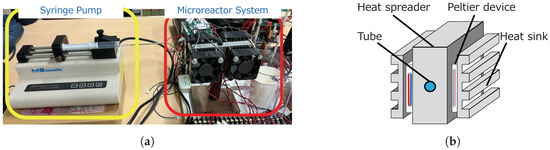
Figure 1.
Experimental system: (a) external view. (b) Schematic diagram of the microreactor system.
3. Problem Statement
This chapter describes the problem setup for this study. In this study, we assume a case in which a tube temperature sensor fails during temperature control of the microreactor system. In this case, we aim to construct a system that allows temperature control to continue without shutting down the entire plant, even during the temperature sensor fault. The following two steps are required:
- A system that determines in real time whether the temperature sensor of a tube is normal or abnormal (fault detection system).
- A control system that compensates for tracking to the reference input in the event of a tube temperature sensor fault (fault-tolerant control systemm)
The fault detection system consists of a One-Class SVM with some of its inputs added to ChangeFinder’s outputs. The discriminant model trained only on normal data learns the relationship between the control input, temperature sensor measurements, and the change-point scores of the temperature sensor measurements by ChangeFinder. If the observed data do not fit the learned relationship, the model discriminates abnormal conditions. This enables fault detection without requiring prior fault data and without specializing in a particular pattern of faults.
The fault-tolerant control system is a nonlinear control system that considers Bounded-Input Bounded-Output (BIBO) stability based on operator theory. The system assumes that an unknown fault factor is added to the normal measured value of the temperature sensor that has failed, and the system operates in such a way that the fault factor is removed. If the control system can remove the fault elements, the temperature of the controlled object can follow the reference input even in the event of an abnormality. However, fault-tolerant control systems require the fault detection system to be activated. Early fault detection is necessary from the standpoint of stability.
Assumed Temperature Sensor Fault Conditions
The following is an explanation of the temperature sensor fault situation assumed in this study. As it is difficult to intentionally cause a sensor fault, the fault is emulated using the measured values of a normal sensor. Various types of sensor faults have been reported [18]. In this study, we consider the case where the sensor deviates from its predetermined position due to a situation such as the sensor being unglued, and shows a measured value that is different from the original temperature of the controlled object. This situation is shown in Figure 2. The fault is represented as a step-like fault element added to the original temperature y for the measured value , as shown in Equations (1) and (2). Note that A is the amplitude of the fault signal, B is the time constant of the fault signal, and is the fault time. The reason for this is explained below. When the position of the sensor suddenly changes as shown in Figure 2b, the ambient temperature of the sensor changes. The Fourier law and thermal radiation create a thermal gradient in the surrounding area. Therefore, a step-like offset change generally occurs while the sensor is moving. Step-like changes also occur due to the thermal inertia of the sensor itself. In temperature, where heat transfer and heat conduction are dominant compared to thermal radiation, the offset change during the fault is expected to be a first-order delay due to the thermal inertia of the sensor. Only fault patterns with such offsets will be considered. The original measured value y is not used in the experiment and is used in all control systems.
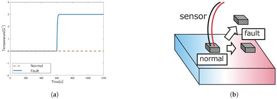
Figure 2.
Assumed temperature sensor fault conditions: (a) deviation of normal and faulty sensor readings from the correct values. (b) Temperature sensor fault condition.
An example of the normal and faulty measured deviation at that time is shown in Figure 2.
4. Modeling
This chapter describes the modeling of the entire microreactor system, including the microreactor(tube) and auxiliary cooling system [19]. Define the multiple area (Part) in the device, as shown in Figure 3. Three Parts are defined for each tube and heat spreader, and the sensor to measure the temperature is installed. The parameters used in the modeling of heat spreaders and tubes are listed in Table 1. The corresponding area parameters in Figure 3 are shown in Table 2. The parameters in Table 1 and Table 2 refer to previous study [19], with some modifications.
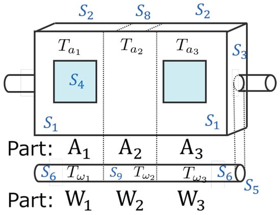
Figure 3.
Area (Part) definition of microreactor system.

Table 1.
Parameters of modeling.
Table 2.
Parameters of area.
4.1. Thermal Models of Heat Spreader
In this section, heat spreaders are modeled based on the laws of heat transfer. The three heat transfer laws used are Fourier’s law, Newton’s cooling law, and Stefan–Boltzmann’s law. The relational equation for heat conduction in Part is obtained using the heat transfer laws and Table 1 and Table 2 as follows. For the left side of the model equation, it is the time derivative of the thermal energy of the Part. The left-hand side shows the total amount of heat energy exchanged by external factors, indicating the heat energy transfer per unit time. Note that since the defined Parts are adjacent to each other, there is interference due to heat transfer. Note that . In addition, and are the heat absorbed from the Peltier device and are discussed in Section 4.3.
4.2. Thermal Model of Tube
Similarly, the thermal model in Part is as follows.
4.3. Heat Absorption by Peltier Device
In this study, the control target is cooled by heat absorption from the Peltier device. For the modeling of the heat spreader performed in Section 3, the control input is the heat absorption from the Peltier device. In this section, the thermal model of the Peltier device is presented and the calculation method of the current input to the experimental device is described.
The heat absorption of the Peltier device is defined as positive. The model of the heat absorption [W] is shown in Equation (9). Similarly, the model of heat dissipation [W] when heat dissipation is defined as positive is shown in Equation (10).
The command value given to the experimental apparatus is the current . When expressed as above, we consider determining the current flowing through the Peltier device based on the heat absorption to be referred to. In this case, the current is obtained by solving the Equation (9) for as follows.
Thermal Model Deformation
Equivalent transformations are performed for the models shown in Section 3, and the transformation is made into an easy-to-handle form. Defining the temperature drop of the controlled object from the outside temperature , the model for the heat spreader is as follows.
In this case, (n = 1, 2, 3) is as follows. The to are constants obtained by Equation transformation.
Similar to the Section 4.2, the equation transformation is performed for the model for the tube Part. Defining the temperature of the drop from the outside temperature to be controlled, the model for the tube is as follows.
In this case, are expressed as follows. to are constants obtained by equation transformation.
5. Control Design
In this chapter, we describe the design of a two-input, two-output temperature control system for the three-division model.
5.1. Right Factorization
Right factorization [16] of the model of the control target described above is performed based on operator theory. Define the heat input including interference in the heat spreader as and the heat input of the tube as . The derived model is subjected to right factorization based on operator theory. First, from Equations (12)–(16), , are shown.
Here, is the temperature of the heat spreader Part . Also, is the temperature of the tube Part . and can be observed from the installed temperature sensors.
Based on operator theory, the plant under control is right factorized into invertible operator and stable operator . The heat spreader is expressed as the following operator.
5.2. Control Design with Right-Coprime Factorization
In this section, the stability of the entire control system is guaranteed by designing a controller based on operator theory for the control target with right factorization [16]. In addition, a controller that compensates for tracking to the reference input in the outer loop is designed to guarantee tracking. The designed controller is shown in Figure 4. Figure 4 shows the control system in vector, for example . Here, the plants to be controlled are and representing heat spreaders and representing tubes. We further define a new operator .
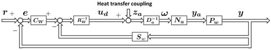
Figure 4.
Control system based on operator theory.
In designing the control system, the controller design is performed under the conditions of , , and . This is because there are only two regions where the amount of heat absorption can be input from the Peltier device: and . Therefore, the system cools and controls by heat transfer from . All other heat transfers that occur between the other are interferences. In this section, the design is performed for the nominal model.
Design the operators according to the Bezout identity in Equation (A12). Designing the operators and so that they satisfy the Beozut identity compensates for the BIBO stability of the nonlinear system. Then and become right-coprime factorizations. In Equation (A12), I is the identity operator and outputs the input signal as it is.
5.3. Fault-Tolerant Control System
In this section, we design a control system that can follow a reference input even in the event of a tube-mounted temperature sensor fault by activating the sensor in the event of the fault. The fault-tolerant control system in this study consists of the fault detection system and the fault signal compensation control system. The control system described is the fault-tolerant control system that is extended from the one-input, one-output fault-tolerant control system of the two-partition model of the previous study [15] to a three-partition model. The fault signal compensation control system used in this study is shown in Figure 5. As in the Section 5.2, only is explained. Here, FD in Figure 5 denotes the fault detection system, which switches to the fault-tolerant control system. Operator is an operator that outputs a signal to compensate for faults and is enabled by the fault detection system.
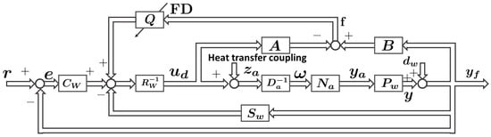
Figure 5.
Fault-tolerant control system.
In the case of a sensor fault, the fault signal is shown as in Equation (30) using the fault element .
Here, when is enabled, the output of the tracking compensation controller is organized as in Equation (31).
In this case, design and so that the left side is and the term including the fault element on the right side is O operator, respectively. Since the model equation for is the same as for Part , the variable uses the temperature sensor measurements of Part .
When operators satisfying the conditions are designed as in Equations (32) and (33), operator is shown as in Equation (34).
Substituting Equations (32)–(34) into Equation (31) again, a relational expression such as Equation (35) is shown.
The relationship in Equation (36) transforms the operator into an operator with a tracking compensation operator . However, to account for thermal disturbances caused by modeling errors of the control target and thermal disturbances caused by thermal transfer with the liquid flowing in the channel, it is transformed like an operator with whose gain of is adjusted separately.
The relationship in Equation (36) removes the fault element from the output, allowing it to follow the reference input even in the event of a fault. Note that when the sensor is determined to be normal.
5.4. Consideration of Coupling Effects
The design of the Section 5.2 and Section 5.3 assumes that the two-input two-output control system is interference-free independent two subsystems. In reality, however, there is interference due to heat transfer between adjacent parts. We consider removing the effect of interference by compensating for this interference with the input from the actuator. The control system considering the removal of couplings is shown in Figure 6.
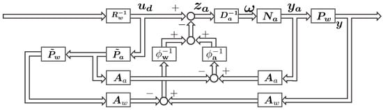
Figure 6.
Control system to remove coupling effects.
Here, , is the heat transfer model of the heat spreader, , is the tube heat transfer model. When there is no effect of coupling, is valid, and the control system design is performed with this as a target. The operators designed in Figure 6 are shown in Equations (38) and (39) below. Here, each operator is assumed to have a bounded signal input and is defined as and . Here, and are design parameters and ), ) is a linear operator such that for any bounded input signal. I is the identity operator.
The equation for is rearranged as in Equation (40).
Since and , the Equation (42) is achieved. This eliminates the effect of coupling.
However, if the tube’s temperature sensor is determined to have failed, the output of the nominal heat transfer model is used instead of the measured value from the temperature sensor for .
5.5. Overall Control System
To summarize the above, the block diagram of the entire control system is shown in Figure 7. Here, in Figure 7, is the operator indicating and is the operator indicating and is the operator indicating .
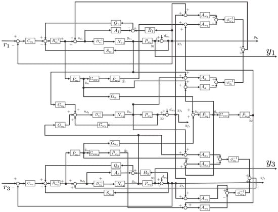
Figure 7.
Overall control system.
6. Fault Detection System
This chapter presents the fault detection system for detecting tube temperature sensor faults. Here, the fault is represented by the control system designed in Section 5.2, shown in Figure 8. The purpose of fault detection in this study is to switch the control loop to the fault-signal-compensating control system described in Section 5.3 in the event of the fault. The goal is to detect the temperature sensor fault in the tube represented by in Figure 8. The using fault detection system is a combination of ChangeFinder and One-Class SVM. One-Class SVM is described in Appendix A and ChangeFinder is described in Appendix B. If the change-points detected by ChangeFinder are considered as anomalies, the system has the advantage of reliably detecting change-points even for minor faults. On the other hand, if the reference input changes during control, it is also detected as a change-point. This has the disadvantage that an abnormality cannot be detected during the transient period until it is tracked again. Abnormality detection by One-Class SVM alone has the advantage that detection is effective even for unknown anomalies. It has the disadvantage that it is difficult to detect small faults; for example, when the distance between the normal data during training and the observed anomaly data is small. Therefore, we aim to construct a system that complements each other’s weak points by adding the output of ChangeFinder to the input of One-Class SVM. The following two processes are required for anomaly detection.
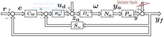
Figure 8.
Representation of temperature sensor faults in control systems.
- Anomaly classification modeling with One-Class SVM. An anomaly discrimination model is constructed by preparing training data and having One-Class SVM learn them. The explanation is given in Section 6.1 and Section 6.2.
- Anomaly detection by anomaly discrimination model. Anomaly detection of acquired real-time data is performed using a discriminant model created in advance. The explanation is given in Section 6.3.
6.1. Creation of Classification Models by Learning
The fault detection system uses a combination of One-Class SVM and ChangeFinder to perform fault detection. In this section, we explain how to construct a classification model for One-Class SVM, which classifies observed data as normal or faulty. One-Class SVM can classify normal classes and abnormal classes by using an abnormality classification model learned using only previously acquired normal data. This makes it effective for plants for which faulty data are difficult to obtain or for which the faulty pattern is unknown. Therefore, training data that have the same dimensions as the data to be input during classification are required during training.
The discriminant model is constructed by training the One-Class SVM with previously observed training data. An overview of the process is shown in Figure 9.
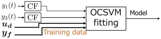
Figure 9.
Training data learning.
As shown in Figure 9, the training data include the input of the heat absorption of the Peltier device, the measured temperature of the tube , and the change-point score of calculated by ChangeFinder. Since the thermal model of the microreactor is a dynamic system, past values affect the current values. In a dynamic system, if a classification model is built using only the current information, the plant characteristics will not be learned correctly and there is a risk of false positives. Therefore, by including time-shifted past data in the learning vector, it is possible to construct the classification model that takes the dynamic system into account. The variable to be trained is as in Equation (43). Note that denotes the change-point score of time-series data by ChangeFinder.
Here, N is the number of training data and is the number of time shifts. In other words, four types of training data are used: input, output, output before one step, and output before two steps. The proposed method detects temperature sensors in Part and Part , whereas the conventional method detects a single temperature sensor located at the center of the tube. In the thermal model of the microreactor, there is interference between adjacent parts, and this is the reason for this detection method.
6.2. Hyperparameter Optimization of One-Class SVM to Improve Classification Performance
One-Class SVM have parameters that must be specified as design parameters during training, called hyperparameters. The two hyperparameters in One-Class SVM are the kernel parameter and the normalization parameter . Hyperparameters have a strong influence on the classification performance of the constructed model, and thus need to be optimized in order to construct a more accurate classification model.
This parameter optimization problem can be treated as an objective function maximization problem with the performance of the constructed classification model as the objective function. In this study, we use a real-coded genetic algorithm [20,21] as one of the optimization methods on a continuous search space. The real-coded genetic algorithm is an optimization algorithm inspired by the evolutionary process of living organisms, in which a real-coded vector is an individual and the value of the objective function is the strength of the individual. Real-coded genetic algorithms are characterized by the fact that they do not explicitly use the gradient of the objective function. Therefore, optimization is possible even for functions for which the gradient of the objective function cannot be obtained, such as the classification performance evaluation in this study. Figure 10 shows the process of hyperparameter optimization using the real-coded genetic algorithm.
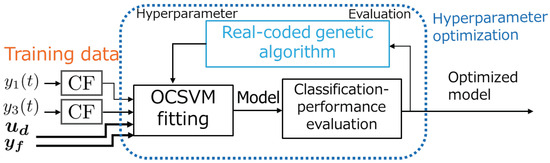
Figure 10.
Hyperparameter optimization process using the real-coded genetic algorithm.
The process of Figure 10 is described in detail as follows.
- Obtain input/output data in advance by experiment as training data.
- Add the expected fault elements to some of the previously acquired input/output data to create test data in the event of the fault.
- Obtain the hyperparameters to be tested using the real-coded genetic algorithm.
- Construct a tentative classification model by training using the training data and the hyperparameters obtained.
- Calculate the classification performance evaluation value from the classification model and test data.
- The real-coded genetic algorithm determines the hyperparameters to try next.
- Repeat the process from 3 to 6 for the product of the number of individuals and the number of generations to obtain the optimized hyperparameters.
Let be the hyperparameter to be tried. The maximization problem for improving the classification performance of this study is shown in Equation (48). is the precision. It is the pattern ratio in which the correct answer is anomalous when it is determined to be anomalous. Similarly, is the recall. It is the proportion of patterns for which the discriminant model was able to discriminate an abnormality out of the patterns for which the correct answer was abnormality. Therefore, the penalty for false positives increases as the value of r is increased.
The above process improves the performance of the classification model by optimizing the hyperparameters of the One-Class SVM.
6.3. Fault and Normal Classification with One-Class SVM and ChangeFinder
In this section, we show how to perform anomaly detection using the discriminant model constructed in Section 6.1. Fault detection is achieved in real time by performing fault detection for each control step. The process for each control step is shown below.
- The temperature is measured by sensors.
- Control inputs and change-point scores are calculated from temperature measurements.
- Similar to Equation (43), a variable X is created for anomaly determination, to be input to OCSVM.
- If classified as faulty in 3, the fault tolerance control system is activated.
7. Simulation Results
In this chapter, the effectiveness of the proposed control and fault detection systems is verified by simulation. Simulations were performed using MATLAB 2023b. One-Class SVM used ocsvm function. ChangeFinder and real-coded genetic algorithms were self-developed. In the simulation, a normally distributed noise with mean 0 and variance 0.0005 is added to assuming the measurement noise of the temperature sensor. The target temperature is (outside temperature - reference input). Simulations were performed for the following two cases. The parameters are also shown in Table 3.
Table 3.
Condition parameters of simulations.
- Part increased from and Part increased from .
- Part W3 increased from .
7.1. Part W1 Increased 3.2 °C from 500 s and Part W3 Increased 3.6 °C from 500 s
Figure 11 shows the results of temperature control using the proposed control system. Figure 12 also shows the results of the real-time fault classification. Figure 11b shows that the value of the fault sensor fluctuates due to the faults that occurred during the 500 s. However, as Figure 11a shows, the temperature of the controlled object continues to track the reference input. The control input jumps up at 500 s due to the sensor fault. However, it returns to the appropriate input by switching to the fault-tolerant control system.
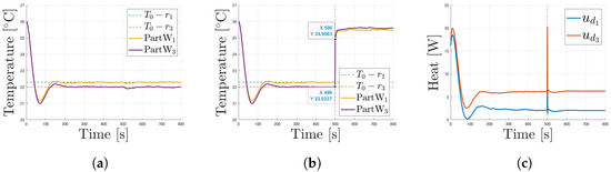
Figure 11.
Simulation results under condition where Part increased from and Part increased from : (a) temperature. (b) Measurements of faulty sensors. (c) Control input.
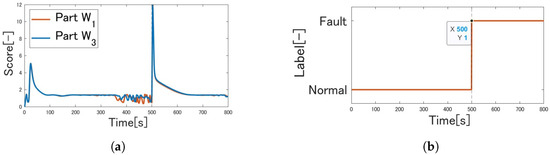
Figure 12.
Simulation results under condition where Part increased from and Part increased from : (a) change-point scores. (b) Classification of fault detection.
Discussing the results for Figure 12a, ChangeFinder’s change-point score jumped at 503 s, 3 s after the fault. Figure 12b shows that One-Class SVM detected the fault at 500 s, the control cycle in which the fault data were first measured; One-Class SVM detected the fault before ChangeFinder’s score jumped. Thus, ChangeFinder contributed little to fault detection. In addition, there were no false positives.
7.2. Part W3 Increased 3 °C from 500 s
Similarly, Figure 13 shows the results of temperature control and Figure 14 shows the results of real-time fault detection. In Figure 13a, the temperature of the controlled object continues to track the reference input. In Figure 13b, the temperature change due to the fault was small. However, ChangeFinder detected the change-point and increased its score at 503 s. One-Class SVM also detected a fault at 503 s, 3 s after the fault occurred, coinciding in time with the increase in ChangeFinder’s change-point score. This confirms the effectiveness of the fault detection system that combines the One-Class SVM input with the ChangeFinder output. No detection was made until the change-point score increased. Thus, it indicates that One-Class SVM alone could not detect faults of this small amplitude. However, as the ChangeFinder change-point score decreased, the fault detection system classified the fault condition as normal.
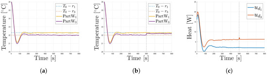
Figure 13.
Simulation results under condition where Part increased from : (a) temperature. (b) Measurements of faulty sensors. (c) Control input.
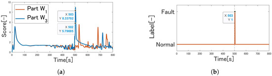
Figure 14.
Simulation results under condition where Part increased from : (a) change-point scores. (b) Classification of fault detection.
8. Experimental Results
In this chapter, we present the results of an experiment on an actual machine. In the experiment, the outside temperature was 22.591 °C. The measured temperature of Part immediately before the start of the experiment is defined as the constant outside temperature. The goal was to cool Part by 3 °C and Part by 4 °C from the outside temperature. The fault element was added to the temperature sensor values, assuming that the fault occurred in 601 s. Table 4 shows the differences in the parameters during the experiment compared to the simulation run. Figure 15 shows the results of the temperature control with the proposed control system. Figure 16 shows the results of the fault classification performed in real time.
Table 4.
Parameters of experiment.
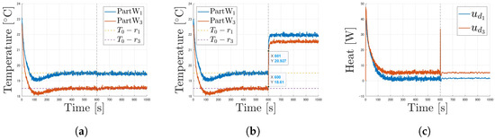
Figure 15.
Experimental results under condition where Part increased from and Part increased from : (a) temperature. (b) Measurements of faulty sensors. (c) Control input.
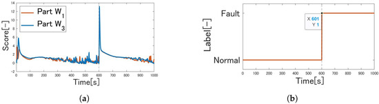
Figure 16.
Experimental results under condition where Part increased from and Part increased from : (a) change-point scores. (b) Classification of fault detection.
As in the experiment, it was confirmed that the system could follow the reference input by switching to the fault-tolerant control system. In addition, fault detection during the 601 s was possible for faults that occurred in the 601 s.
Comparison of Simulation and Experiment
The simulation results shown in Section 7.1 are compared with the experiment results. However, since the target temperatures and fault requirements are different, the comparison is made based on the average absolute error from the reference input after the time of the fault. Specifically, the simulation is calculated using temperatures from 500 to 800 s, while the experiment is calculated using results from 601 to 1000 s. As shown in Table 5, the mean absolute error is smaller for the simulation. Therefore, the simulation results are superior in this comparison.
Table 5.
Comparison of simulation and experiment.
9. Conclusions
In this study, the fault-tolerant control system was designed for the MIMO system that controls the temperature of two regions of the microreactor system. This extends the fault-tolerant control system, which was effective for only one region in previous studies. In addition, the fault detection system combining One-Class SVM and ChangeFinder was applied to detect faults; for training the One-Class SVM, the evaluation function for the classification model was created, and the hyperparameters were optimized by the real-coded genetic algorithm. Finally, the effectiveness of the system was verified through simulations and experiments. The fault detection system combining One-Class SVM and ChangeFinder detected faults even when the amplitude of the fault elements was small. The results show that the system is more effective than One-Class SVM alone in detecting failures in microreactor systems.
Author Contributions
Y.M. used a combination of One-Class SVM and ChangeFinder for training to create the fault classification model for temperature sensors. Parameter optimization of the fault classification model was performed using a real-coded genetic algorithm. In addition, we proposed a method to extend the fault-tolerant temperature control system of the microreactor to a MIMO fault-tolerant temperature control system, and proposed a control system combined with fault classification. Simulation and actual experiments were also conducted and this paper was written. M.D. suggested technical support and gave overall guidance on the paper. All authors have read and agreed to the published version of the manuscript.
Funding
This research received no external funding.
Institutional Review Board Statement
Not applicable.
Informed Consent Statement
Not applicable.
Data Availability Statement
Data are contained within the article.
Conflicts of Interest
The authors declare no conflicts of interest.
Appendix A. One-Class SVM
One-Class SVM, a one-class classification method [22,23], is described. The algorithm is described below. First, the training data are prepared, and the inner product of the projection data by is defined as a kernel function as in Equation (A1). In this study, the RBF kernel is used.
Assuming that the normal and abnormal data are linearly separable in the high-dimensional space after mapping, the separation plane is expressed as Equation (A2) using the weight coefficient and bias .
To allow for misclassification, a slack variable is introduced. In this case, we consider maximizing the distance from the origin with respect to the classification plane. Converting the maximization problem into a minimization problem, it is shown as follows, including the constraints using the normalization parameter .
Also, introducing the new variables and Equation for the minimization problem, the Lagrangian function is shown as follows.
The minimization problem becomes a -only problem, as follows.
Using the final optimized Lagrange multiplier , the decision function for the unknown data are as follows.
The outlier-likeness of unknown input patterns mapped to a higher-dimensional space increases as the distance from the origin is shortened. Therefore, input patterns that are placed closer to the origin than the classification plane do not belong to a class and are judged to be outliers.
Appendix B. ChangeFinder
ChangeFinder is an algorithm that computes the likelihood of change-points in time-series data. A change-point is a time when the behavior of time-series data changes significantly. In this study, we use the SDAR model, which has a forgetting function and can deal with non-stationary data to some extent. The SDAR model is effective in detecting essential change-points because it suppresses the increase in change-point scores caused by noise through two-stage learning [14]. The calculation procedure for each time-series data is as follows.
- Reading time-series data .
- Learning SDAR model and computing probability density function .
- Calculation of outlier scores during one-step learning
- Smoothing of scores and derivation of moving average using smoothing width .
- Apply SDAR to and calculate the probability density function for two-step learning.
- Smoothing again yields the moving average at time t as the change-point score.
The higher the score, the greater the degree to which it is a change point. The following is a description of the SDAR algorithm.
- Read the time-series data .
- The computed estimator is used to update the estimate of the statistic to be used. Where is the forgetting coefficient. The higher the forgetting coefficient, the greater the influence of the past state.
- Solve the Yule–Walker equation for .
- Compute the variables used in the score calculation.
References
- Ehrfeld, W.; Hessel, V.; Löwe, H. Microreactors: New Technology for Modern Chemistry; Wiley/VCH: Weinheim, Germany, 2000. [Google Scholar]
- Yao, X.; Zhang, Y.; Du, L.; Liu, J.; Yao, J. Review of the applications of microreactors. Renew. Sustain. Energy Rev. 2015, 47, 519–539. [Google Scholar] [CrossRef]
- Burns, J.R.; Ramshaw, C. Development of a Microreactor for Chemical Production. Chem. Eng. Res. Des. 1999, 77, 206–211. [Google Scholar] [CrossRef]
- Tamagawa, O.; Muto, A. Development of cesium ion extraction process using a slug flow microreactor. Chem. Eng. J. 2011, 167, 700–704. [Google Scholar] [CrossRef]
- Zhao, D.; Tan, G. A review of thermoelectric cooling: Materials, modeling and applications. Appl. Therm. Eng. 2014, 66, 15–24. [Google Scholar] [CrossRef]
- Najafi, H.; Woodbury, K.A. Optimization of a cooling system based on Peltier effect for photovoltaic cells. Sol. Energy 2013, 91, 152–160. [Google Scholar] [CrossRef]
- Deng, M.; Inoue, A.; Goto, S. Operator based Thermal Control of an Aluminum Plate with a Peltier Device. Int. J. Innov. Comput. Inf. Control 2008, 4, 3219–3229. [Google Scholar]
- Takahashi, K.; Wen, S.; Sanada, M.; Deng, M. Nonlinear cooling control for a Peltier actuated aluminum plate thermal system by considering radiation heat transfer. In Proceedings of the 2012 International Conference on Advanced Mechatronic Systems, Tokyo, Japan, 18–22 September 2012; pp. 18–23. [Google Scholar]
- Hwang, I.; Kim, S.; Kim, Y.; Seah, C.E. A survey of fault detection, isolation, and reconfiguration methods. IEEE Trans. Control Syst. Technol. 2009, 18, 636–653. [Google Scholar] [CrossRef]
- Isermann, R.; Balle, P. Trends in the application of model-based fault detection and diagnosis of technical processes. Control Eng. Pract. 1997, 5, 709–719. [Google Scholar] [CrossRef]
- Gao, Z.; Cecati, C.; Ding, S.X. A Survey of Fault Diagnosis and Fault-Tolerant Techniques—Part I: Fault Diagnosis with Model-Based and Signal-Based Approaches. IEEE Trans. Ind. Electron. 2015, 62, 3757–3767. [Google Scholar] [CrossRef]
- Zhang, W.; Xu, D.; Enjeti, P.N.; Li, H.; Hawke, J.T.; Krishnamoorthy, H.S. Survey on Fault-Tolerant Techniques for Power Electronic Converters. IEEE Trans. Power Electron. 2014, 29, 6319–6331. [Google Scholar] [CrossRef]
- Venkatasubramanian, V.; Rengaswamy, R.; Kavuri, S.N.; Yin, K. A review of process fault detection and diagnosis: Part III: Process history based methods. Comput. Chem. Eng. 2003, 27, 327–346. [Google Scholar] [CrossRef]
- Takeuchi, J.; Yamanishi, K. A Anifying Framework for Detecting Outliers and Change Points from Time Series. IEEE Trans. Knowl. Data Eng. 2006, 18, 482–492. [Google Scholar] [CrossRef]
- Ogihara, Y.; Deng, M. Operator-based Nonlinear Fault Detection and Fault Tolerant Control for Microreactor using One-Class SVM. Int. J. Adv. Mechatron. Syst. 2020, 8, 109–115. [Google Scholar] [CrossRef]
- Deng, M.; Inoue, A.; Ishikawa, K. Operator-based nonlinear feedback control design using robust right coprime factorization. IEEE Trans. Autom. Control 2006, 51, 645–648. [Google Scholar] [CrossRef]
- Furukawa, Y.; Deng, M. SVM-based fault detection for double layered tank system by considering ChangeFinder’s characteristics. Int. J. Adv. Mechatron. Syst. 2022, 9, 185–192. [Google Scholar] [CrossRef]
- Li, D.; Wang, Y.; Wang, J.; Wang, C.; Duan, Y. Recent advances in sensor fault diagnosis: A review. Sens. Actuators A Phys. 2020, 309, 111990. [Google Scholar] [CrossRef]
- Nishizawa, K.; Deng, M. Operator-based Nonlinear Modeling and Control of Microreactor Considering Symmetry. In Proceedings of the 2021 IEEE International Conference on Networking, Sensing and Control (ICNSC), Xiamen, China, 3–5 December 2021; pp. 1–6. [Google Scholar]
- Tsutsui, S.; Yamamura, M.; Higuchi, T. Multi-parent recombination with simplex crossover in real coded genetic algorithms. In Proceedings of the 1st Annual Conference on Genetic and Evolutionary Computation, Orlando, FL, USA, 13–17 July 1999; pp. 657–664. [Google Scholar]
- Eshelman, L.J.; Schaffer, J.D. Real-Coded Genetic Algorithms and Interval-Schemata. Found. Genet. Algorithms 1993, 2, 187–202. [Google Scholar]
- Schölkopf, B.; Platt, J.C.; Shawe-Taylor, J.; Smola, A.J.; Williamson, R.C. Estimating the support of a high-dimensional distribution. Neural Comput. 2001, 13, 1443–1471. [Google Scholar] [CrossRef] [PubMed]
- Yin, S.; Zhu, X.; Jing, C. Fault detection based on a robust one class support vector machine. Neurocomputing 2014, 145, 263–268. [Google Scholar] [CrossRef]
Disclaimer/Publisher’s Note: The statements, opinions and data contained in all publications are solely those of the individual author(s) and contributor(s) and not of MDPI and/or the editor(s). MDPI and/or the editor(s) disclaim responsibility for any injury to people or property resulting from any ideas, methods, instructions or products referred to in the content. |
© 2024 by the authors. Licensee MDPI, Basel, Switzerland. This article is an open access article distributed under the terms and conditions of the Creative Commons Attribution (CC BY) license (https://creativecommons.org/licenses/by/4.0/).