Abstract
Variability in manufacturing processes must be properly monitored and controlled to avoid incurring quality problems; otherwise, the probability of manufacturing defective products increases, and, consequently, production costs rise. This paper presents the development of a methodology to locate the source(s) of variation in the manufacturing process in case of a statistical deviation so that the user can quickly take corrective actions to eliminate the source of variation, thus avoiding the manufacture of out-of-specification products. The methodology integrates the multivariate cumulative sum control chart and the multilayer perceptron artificial neural network for the detection and interpretation of the source(s) of variation generated in the manufacturing processes. A case study was carried out with a printed circuit board manufacturing process, and it was possible to classify the origin of the variation with a sensitivity of 92.41% and specificity of 91.16%. The results demonstrate the viability of the proposed methodology to monitor and interpret the source of statistical variation present in production systems.
1. Introduction
The success of a company depends mostly on the quality and productivity of the goods or services it produces, so quality monitoring has become a vitally important tool for companies to grow and remain competitive in the market [1]. Currently, manufacturing industries use statistical process control (SPC) to improve the quality of their products and to monitor the variability of the production process [2]. The variability inherent to the manufacturing process is known as natural or random causes; on the other hand, when the variability is increased by predictable effects, it is known as special or assignable causes. With respect to the state of a process, it is said that a process is under control when only natural or random causes exist [3]. Importantly, early detection of assignable causes always leads to rapid implementation of preventive actions and process improvements, which can usually reduce production losses [4].
Control charts are tools of statistical process control that are widely applied to effectively detect the occurrence of assignable causes, since they provide graphical information about the state of the process, where the values of statistical variables are represented for a series of successive samples [5]. In today’s production processes, there are usually characteristics that have a joint and interrelated influence on the final quality of the products, and therefore it is vital to monitor each characteristic simultaneously using multivariate statistical process control (MSPC) techniques. In this way, not only will the effect of each characteristic on quality be analyzed, but also the effect of the interactions between them is considered [6]. Hotelling’s T2 chart is the most widely researched and applied control procedure for monitoring multiple correlated quality characteristics in a production process. However, to detect variations with magnitudes smaller or equivalent to one standard deviation in the vector of averages with greater sensitivity than the Hotelling T2 chart, multivariate cumulative sum (MCUSUM) and exponentially weighted moving average (MEWMA) control charts have been proposed, both control charts incorporate information from previous periods of the process allowing the increase in the detection capability of the chart in the face of variations in the process [7].
It should be noted that one of the disadvantages of multivariate statistical control charts is the lack of a mechanism focused on identifying the source of variation that generates a signal out of statistical control in the chart [8]. The negative consequence caused by the lack of interpretation of the warning signals produced in multivariate control charts is the loss of time and resources invested to locate the source of variation within the production system, resulting in a loss of quality and competitiveness in the organization. To facilitate the interpretation of out-of-control signals in multivariate charts or to increase their sensitivity to variability in manufacturing processes, several proposals have been made in the literature to complement the practical use of the charts; see Table 1.

Table 1.
Literature review.
As can be seen in the literature review, the most used multivariate control charts are the MCUSUM and MEWMA for their sensitivity in detecting small changes in the process. As for a method that analyzes out-of-control signals in univariate charts or pattern recognition, artificial neural networks such as the multilayer perceptron and support vector machine have been used for their generalization capacity. However, the integration of multivariate graphs with memory for process monitoring and variability analysis using multilayer perceptron artificial neural network and support vector machines (SVM) is not addressed.
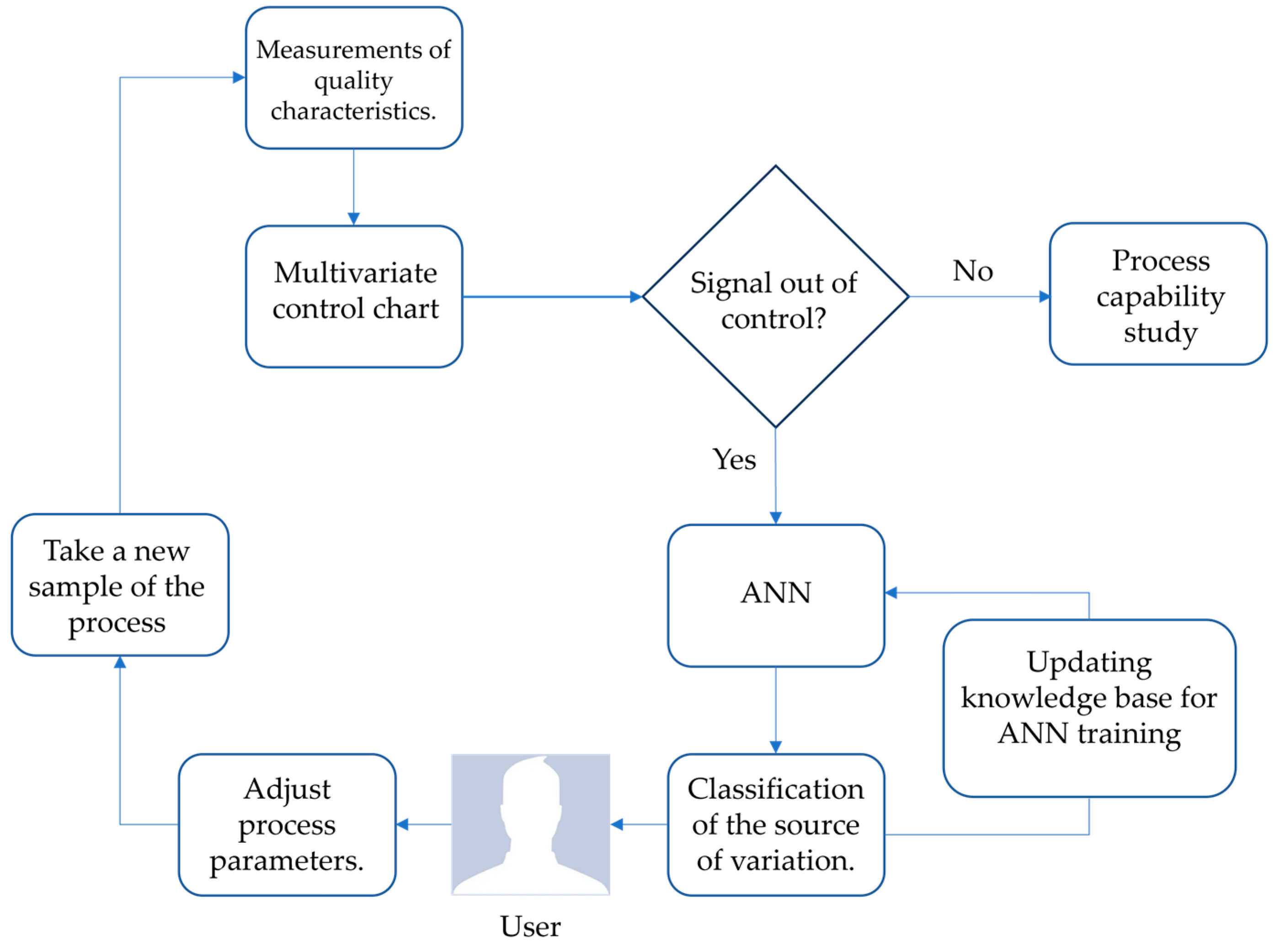
This research work proposes the development of an efficient methodology for the interpretation and analysis of out-of-control signals in a multivariate production system working in two phases. The first phase is carried out by the multivariate control chart that responds to the task of monitoring and surveillance of quality in the production system, and once a mismatch occurs in the process and an out-of-control signal is presented in the multivariate chart, phase two is used. The second phase is aimed at analyzing the source of variation by means of the artificial neural network (ANN). In this way, the procedure will allow the users of the production system to locate the variable(s) that cause(s) the lack of control in the process, being able to employ corrective actions that manage to reduce the production of out-of-specification products early on. The multivariate control and classification methods will be defined from experiments where they demonstrate their efficiency for the task of monitoring and interpretation of the variation generated in the manufacturing processes. Figure 1 shows the steps to develop the proposed methodology.
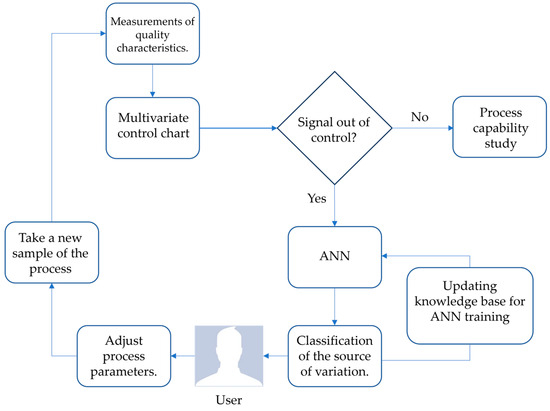
Figure 1.
Proposed methodology.
After an introduction and bibliographic review of the subject to be dealt with in Section 1, the paper is organized as follows: Section 2 and Section 3 are composed of the materials and methods used for the development of the proposed methodology, respectively. The results of the experiments and validation are shown in Section 4. Finally, the discussion of the procedure generated is presented in Section 5.
2. Materials
The application case for the research was carried out in a printed circuit board (PCB) production system; however, the methodology can be implemented in any production system where more than one quality characteristic of its products is monitored [18]. There is a sequence of operations involved in the PCB assembly process: The first step of the PCB assembly process is to apply solder paste to the printed circuit board, and the paste is applied through a printing machine whose function is to regulate the application process to ensure the amount of solder placed on the board. Subsequently, the electronic components are placed on the PCB by means of coordinates. Once all the components are in place, the next step in the PCB assembly process is to solder them. Finally, the PCBs undergo inspection and quality control [19]; see Figure 2.
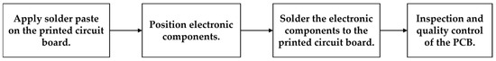
Figure 2.
Printed circuit board (PCB) assembly process.
The first challenge for PCB fabrication is to control the variation in the amount of paste applied to the printed circuit board, where even small variations in the application operation can affect the quality and reliability of the solder connections. Specialized solder paste inspection (SPI) equipment is used to monitor the paste application in the manufacturing process, and thus it is possible to measure the volume, area, and height of the solder deposit. Measuring the volume, area, and height of the paste can allow the manufacturer to predict the quality and long-term reliability of the solder joints on the PCB [20].
The methodology developed was implemented for the monitoring and interpretation of out-of-control signals generated in the solder paste application process. Three quality characteristics are continuously monitored in the operation and each of them presents different manufacturing conditions. Table 2 shows the solder paste specifications for a component (resistor) to be soldered to the printed circuit board.
Table 2.
Solder paste specifications for an electronic component.
2.1. Multivariate Control Charts
The procedure to construct the MCUSUM and MEWMA control charts starts with the calculation of central tendency and dispersion statistics for p quality characteristics, when the manufacturing process is under statistical control [21]. As a measure of central tendency, the vector of sample means is defined from Equation (1); it is the vector formed by the p individual means of the monitored quality characteristics:
The sample covariance matrix associated with the vector of means is determined by Equation (2). The matrix is symmetrical, with the variances of the variables appearing on its diagonal and the covariances between each pair of variables of the quality characteristics outside it [22].
The vector of means and the covariance matrix are the starting point for multivariate statistical control, since multivariate control charts are only valid when the variable follows a multivariate normal distribution [23], whose density is given by Equation (3).
where is a vector of components and is a symmetric dimension matrix.
2.1.1. MCUSUM Control Chart
The structuring of the control chart begins with the extraction of a new sample of measurements for each of the quality characteristics monitored in the process, which will allow us to verify the statistical stability of the manufacturing system [24]. The MCUSUM statistic is calculated from Equation (4).
where
Being
where is the vector of quality characteristics measurements, is the vector of means, is the covariance matrix, is a constant (0.5), and .
The out-of-control signal is generated when , where h is the control limit of the chart (UCL). According to [25], the values of k and h conducive to proper efficiency of the MCUSUM graph are 0.5 and 5.5, respectively.
2.1.2. MEWMA Control Chart
To develop the MEWMA graph, it is necessary to solve Equation (7); in this equation, the depth level of the graph memory will have been defined.
where is the vector of quality characteristics measurements, = is the vector of means, and is memory depth.
The mathematical model shown in Equation (8) represents the magnitude of the statistic to be plotted [26].
where represents the difference between the current measurement and the vector of means and is the covariance matrix with memory.
2.2. Multilayer ANN Perceptron
The multilayer perceptron ANN is a tool used to classify and model nonlinear behaviors such as those commonly occurring in the industrial sector. The multilayer perceptron ANN architecture consists of an input layer, an arbitrary number of hidden layers, and an output layer. Each of the neurons in the hidden or output layers receives an input from neurons in the previous layer, but there are no lateral connections between neurons within each layer [27]. The input layer contains as many neurons as categories corresponding to the independent variables to be represented, and the output layer corresponds to the response variable. The operation of the ANN consists of two important tasks: training and testing. Training an ANN is a process that modifies the value of the weights and biases associated with each neuron so that the ANN can, from data presented in the input layer, generate an output. The test task consists of measuring the level of error generated by the ANN when producing an output with data from the problem that were not included in the training task [28]. The multilayer perceptron artificial neural network operates as a function of Equation (9).
where is the weight factor that the network assigns to the input information, corresponds to the input signal, and is the bias determined by the network.
The activation function is expressed as in Equation (10) and provides an output in the interval [−1, +1].
2.3. Support Vector Machine
Support Vector Machine (SVM) is a supervised machine learning algorithm applicable to classification problems and is based on the hyperplane concept [29]. The concept of separation hyperplane does not generalize naturally for more than two classes (), so strategies have been developed to apply this classification method to situations with , among which the one-versus-one situation has been highlighted. This method constructs SVMs, each comparing one of the classes against the remaining classes, obtaining a classification hyperplane for each class. A test observation is classified using each of the SVMs and the number of times this observation is assigned to each of the classes is counted. The final predicted class will be the one to which the observation has been assigned in most of the SVMs [30].
3. Methods
This section consists of the development of the different materials used for the construction of the proposed methodology; the methods contemplate the detailed description of the approach and execution of the multivariate control charts, artificial neural network multilayer perceptron, and support vector machine.
3.1. Development of Multivariate Control Charts
To exemplify the construction of the multivariate control charts MCUSUM and MEWMA, 30 observations are shown for each of the variables from data taken from production, which will allow estimating the vector of means and covariance matrix. See Table 3.
Table 3.
Quality characteristic measurements.
The vector of means and covariance matrix are defined in Equations (11) and (12), respectively.
To verify the multivariate normality assumption, the Mardia test is applied. According to the results, the sample follows a multivariate normal distribution with a significance level of 0.05, skewness of (0.0774) > (0.05), and kurtosis of (0.8341) > (0.05). See Table 4.
Table 4.
Multivariate normal distribution test.
To continue with the development of the multivariate control chart, a new sample of measurements is extracted for each of the quality characteristics monitored in the process, which will allow verifying the statistical stability of the manufacturing system, in this case, the supervision in the application of solder in the assembly process of the electronic cards. Table 5 shows the sample that will be used to exemplify the development of the MCUSUM and MEWMA control chart.
Table 5.
Measurements to develop the MCUSUM chart.
The detailed procedure for calculating the MCUSUM control chart statistics is shown. We take, as an example observation number, one of the samples and start with the difference between the sample and the vector of means; see Equation (13).
Substitute in Equation (6) to obtain the value of Equation (14) and evaluate the case in Equation (5).
Equation (15) is solved, obtaining Equation (16).
Finally, the multivariate MCUSUM statistic is calculated by substituting in Equation (4) and the statistic for observation number is obtained; see Equation (17).
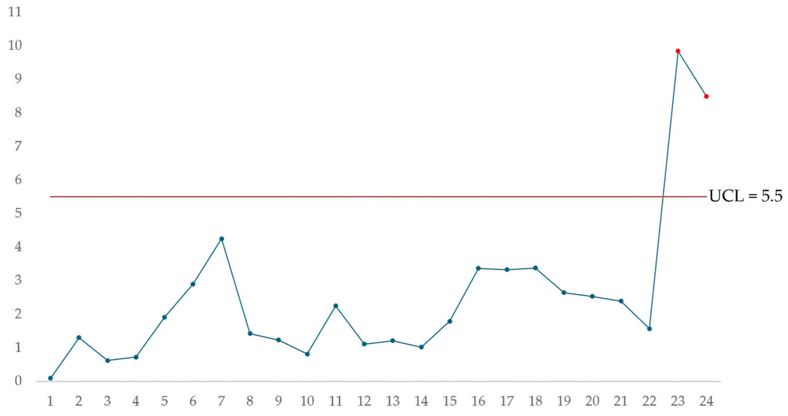
Table 6 shows the MCUSUM statistics for each of the observations used to construct the control chart; the procedure is the same as shown above for each observation. Figure 3 shows the MCUSUM control chart resulting from plotting the statistics and the control limit. The MCUSUM chart shows that samples twenty-three and twenty-four generate an out-of-control signal in the welding application process; these samples should be analyzed to identify the nature of the variation and correct the statistical lack of control of the process.
Table 6.
MCUSUM statistics.
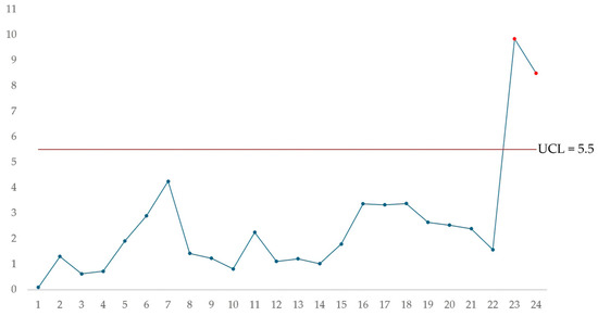
Figure 3.
MCUSUM multivariate control chart.
The structuring of the MEWMA control chart begins by defining the depth value for the chart memory; for this case, a value of (λ = 0.1) was taken. The estimation of the statistic starts with the substitution of the initial data in Equation (7), and the solution is shown in Equation (18)
The MEWMA statistic for the first measurement is obtained by solving Equation (19).
The control limit was defined according to the value of p = 3, λ = 0.1, and an average run length (ARL) of ARL = 200; therefore, the control limit is equal to (10.81). Table 7 presents the MEWMA plotted statistics. Figure 4 shows the MEWMA control chart after plotting the statistics and the control limit.
Table 7.
MEWMA statistics.
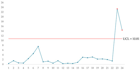
Figure 4.
MEWMA multivariate control chart.
For the solder application process on the PCB boards, both multivariate control charts detected out-of-control signals, and now the person responsible for the process must correct the problem in the production system that causes the variation, which implies time, resources and a complementary analysis. Next, the development of the proposed system based on the multilayer perceptron artificial neural network to detect which of the analyzed variable(s) is (are) out of control automatically is discussed.
3.2. Development of the Artificial Neural Network Multilayer Perceptron
As mentioned above, the operation of the artificial neural network multilayer perceptron consists of two significant tasks: training and testing. The data set generated for the training phase is integrated by simulating one hundred events with variation in the vector of means for each of the seven possible categories with levels of 0.5σ, 1.5σ, and 2.5σ, building a training matrix of size [3 × 2100]. Table 8 shows how to set up the training with a variation of 0.5σ in the vector of means for the seven possible categories of the industrial application case under study. The objective values required by the artificial neural network to perform the task of classification and recognition of the dissimilar categories are assigned according to the hyperbolic tangent activation function, which can take continuous values in the range [−1, 1] and are assigned equidistantly in the domain of the function.
Table 8.
ANN training.
The test matrix is developed from simulated data from measurements obtained from the manufacturing system; the data are classified in two hundred vectors that present different magnitudes of variation in each of the variables, and the magnitude of variation contemplated is 1σ, 2σ, and 3σ. Since there are seven possible categories in the response variable, a matrix of [3 × 4200] is generated. Once the training and test sets have been developed, the ANN architecture is built. The efficiency of the proposed method for the analysis of out-of-control signals will depend directly on the accuracy with which the artificial neural network classifies the changes that occurred in the different variables during the manufacturing process. To achieve adequate efficiency, it is necessary to establish correct operating parameters in the ANN; to achieve this objective, an experiment was carried out. The ANN topologies proposed in Table 9 are architectures that adequately classify the values established during the training phase, so a statistical parameter such as the mean square error (MSE) was used to determine the topology that should be selected for the test phase and subsequently solve the classification task.
Table 9.
ANN topologies developed for the training phase.
Artificial neural network architectures were developed dynamically by constructing an algorithm based on exhaustive experimentation conditioned on cycles to evaluate the total number of possible combinations of topologies. The first parameter considered is the number of neurons in the hidden layer with an interval of [5, 2000]. The second parameter is the learning rate with an increment factor of 0.001 [0.005, 0.9]. The allowed error was set to only two possibilities, 1 × 10⁻⁴ and 1 × 10⁻⁵. Finally, training was scheduled to pause via the down gradient method if the error function did not improve by at least 0.0001 over one hundred iterations. For each architecture, its output was recorded in a database to proceed to calculate the mean square error against the previously established target values and this was the mechanism for the selection of the topologies. The advantage of the proposed procedure is to ensure a global minimum and avoid falling into local minima.
Table 10 shows the topology of the ANN selected to carry out the classification task of the variable(s) generating variation in the manufacturing system to establish an efficient multivariate statistical process control analysis based on artificial intelligence. Once the weights and biases with which the ANN operates have been obtained, the classification task is automatic, since it only involves matrix operations.
Table 10.
Selected topology.
When a signal out of statistical control occurs, it is vital to detect the variable(s) causing the variation in the process to correct the operating conditions early. The multilayer ANN classification scheme is based on synaptic weights and bias generated from the iterative training process, exemplified by observation twenty-three.
W1: synaptic weights of the first layer (1492 × 3):
b1: bias of the first layer (1 × 1492):
W2: synaptic weights of the hidden layer (1 × 1492):
b2: bias of the hidden layer (1 × 1):
Substituting the values of the measurements that generate the out-of-control signal in the process and the input layer matrices in Equation (9), Equation (20) is obtained, generating as a result a vector with dimensions of [1 × 1492].
For each value obtained from the vector, is substituted in Equation (10), resulting in a vector [1 × 1492]; see Equation (21).
Finally, the response issued by the methodology is generated by substituting in the general ANN function the matrices of weights , bias , and the transpose of the resulting vector of the first layer see Equation (22).
The variable corresponds to the value that the ANN assigned to the measurement that caused the out-of-control point in the multivariate control charts, According to the multilayer ANN perceptron output, sample twenty-three was associated with category number four of the seven possible categories since it is the closest value to the ANN classification. For this reason, the ANN result suggests that the variable volume and area present an excessive variation. As can be seen in Table 4, the data for the quality characteristics volume (0.09991) and area (0.76860) are not within specification; see Table 1. Therefore, the ANN correctly analyzed the system variation by identifying the source of variation.
One purpose of the research is to compare the results obtained by the multilayer perceptron ANN, and therefore a support vector machine was developed since it is important to highlight that according to the literature review, both classification approaches have been employed for the analysis of variation in manufacturing systems.
3.3. Development of Support Vector Machine
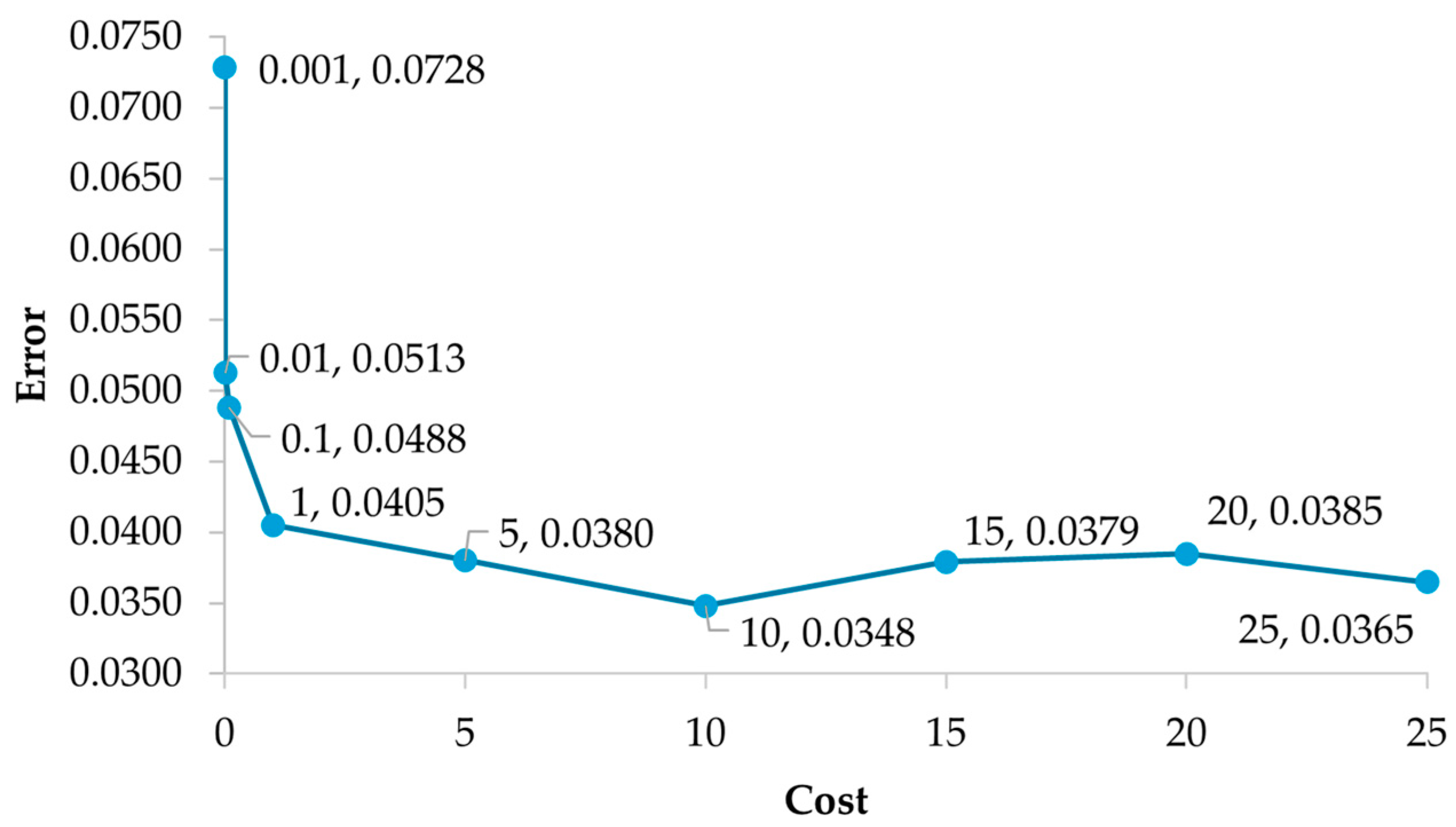
For the development of the support vector machine, use was made of the same training and test sets used in the multilayer perceptron ANN since it also works under a supervised training approach. It is important to consider that the classification of out-of-control signals in multivariate control charts is of the nonlinear type, so a polynomial kernel function was implemented with the one-versus-one method, since a scenario where there are more than two categories is addressed. For the construction of the SVM, it is vital to consider that the hyperparameter cost (C) controls the balance between bias and variance; it is a concept that allows us to understand the ability of the SVM when faced with data that have not been used in the training phase, i.e., its generalization capacity [31]. To select an optimal cost value, different values were evaluated by cross-validation [ 0.001, 0.01, 0.1, 1, 1, 5, 10, 15, 20, 25]. The cost value resulting in the lowest validation error is 10 (0.0348); see Figure 5. The degree of the generated model is the third and the number of support vectors is 203.

Figure 5.
Cost value vs. validation error.
4. Results
To test the performance of the multilayer perceptron artificial neural network and SVM for classifying and analyzing the source of variation detected by the control charts, their results were compared based on the performance measures: sensitivity, specificity, and accuracy (Equations (23)–(25), respectively). The probability of not incurring a type II error, (1 − β), is known as the power of the test, equivalent to the sensitivity. The probability of not making a type I error, (1 − α), is known as the efficiency of the test, equivalent to the specificity. The degree of accuracy of a test is defined as the proportion of cases where the result is correct [32].
where TP is true positive, FP is false positive, TN is true negative, and FN is false negative.
The results generated by the ANNs used for the analysis of the statistical variation generated in the solder paste application process when introducing the test matrix are shown in Table 11.
Table 11.
Results generated by the artificial neural networks.
According to the results obtained, the multilayer perceptron ANN presents a higher average efficiency for the various levels of variation compared to the SVM ANN. The multilayer perceptron ANN achieves an average accuracy of 96.45% to detect changes with magnitudes averaging one standard deviation in the quality characteristics of the manufacturing process, which translates into a strict monitoring of the process. Regarding the accuracy of the multilayer perceptron ANN to classify variation increments in two and three standard deviations in the operation of applying solder paste, the accuracy increases to 96.97% and 98.25%, respectively. The increase in accuracy is logical, since, by incurring a greater variation within the manufacturing process, the measurement that would originate such a warning signal in the control chart would be further away from the average, and, consequently, it would be easier to classify through the ANN.
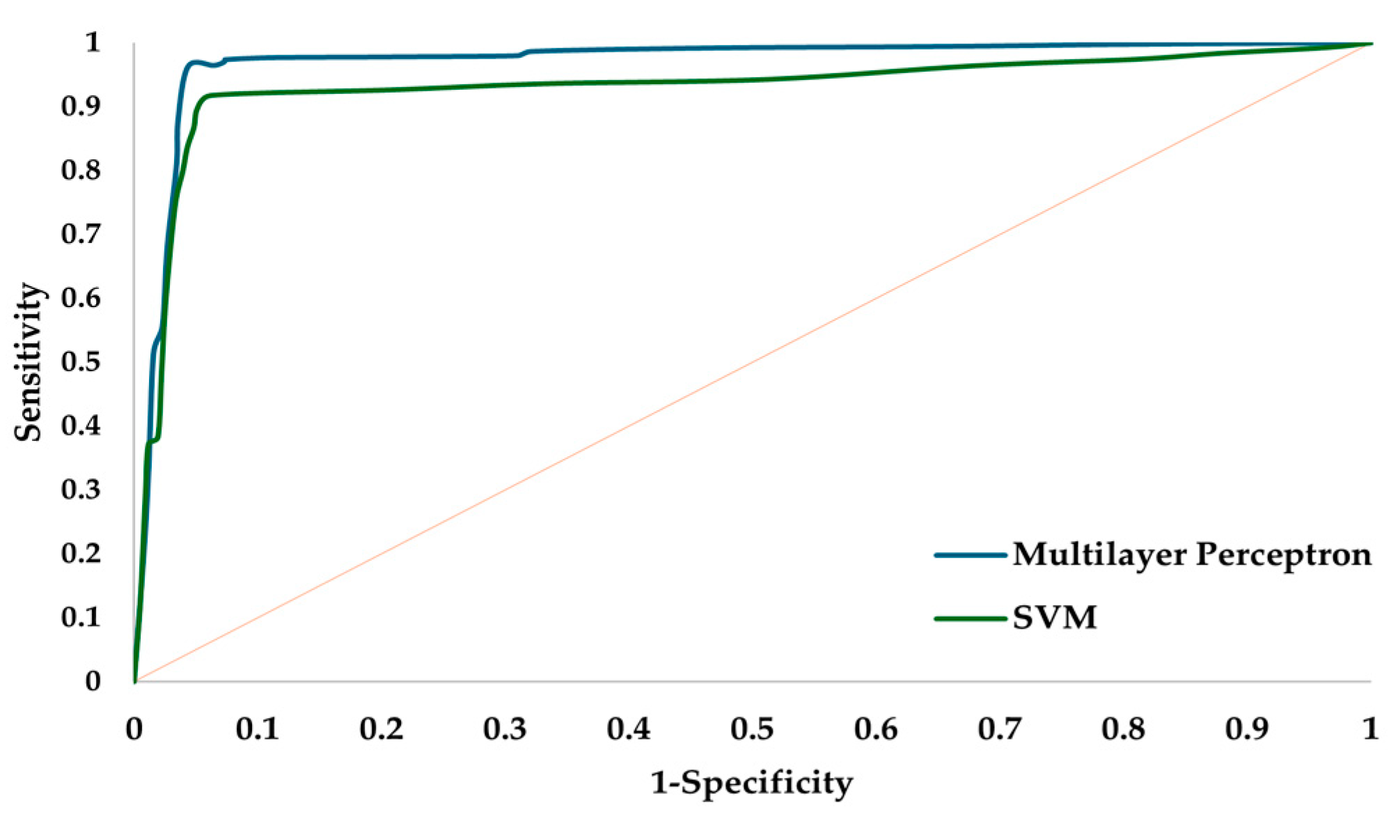
The ROC (receiver operating characteristic curve) analysis applied to the multilayer perceptron artificial neural network and SVM allows us to determine through the Youden index the highest sensitivity and specificity to classify the source of variation generated in the PCB manufacturing process; see Figure 6. The area under the curve (AUC) estimates the probability that the artificial neural network model can correctly discriminate the source of variability; see Table 12.

Figure 6.
ROC analysis test phase.
Table 12.
AUC, 95% confidence interval, and Youden index.
Validation of Classification Models
After testing the developed methodology with simulated data, a validation phase is continued with data obtained directly from the process. A validation matrix of size [3 × 2100] was formed where 100 measurements were included for each of the seven classes with magnitudes of variation classified as 1σ, 2σ, and 3σ. The first phase of validation corresponds to the multivariate control charts to which the task of monitoring and surveillance of quality in the production system corresponds. Table 13 shows the level of efficiency of each of the control charts to detect the variations occurring in the process and concentrated in the validation matrix, where it is shown that the chart with the highest efficiency to detect the variability generated in the solder paste application operation is the MCUSUM chart.
Table 13.
Comparison of control charts.
To validate the use of the artificial neural network focused on the analysis of the source of variation occurred in the process, it is important to evaluate its performance in conjunction with the multivariate control chart. Table 14 shows the probability of detecting and interpreting the source of variation in the solder paste application operation. According to the results, the integration of the MCUSUM control chart and the multilayer perceptron ANN gives the best results.
Table 14.
Integration of control charts and artificial neural networks.
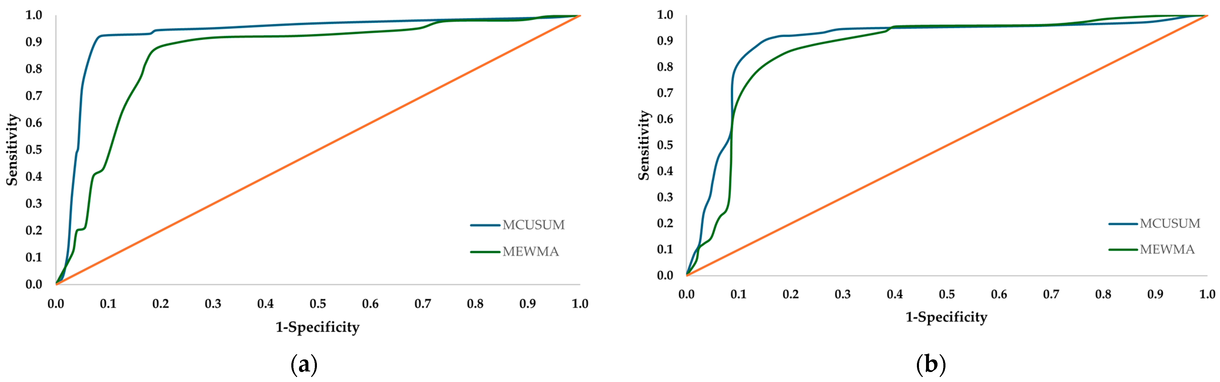
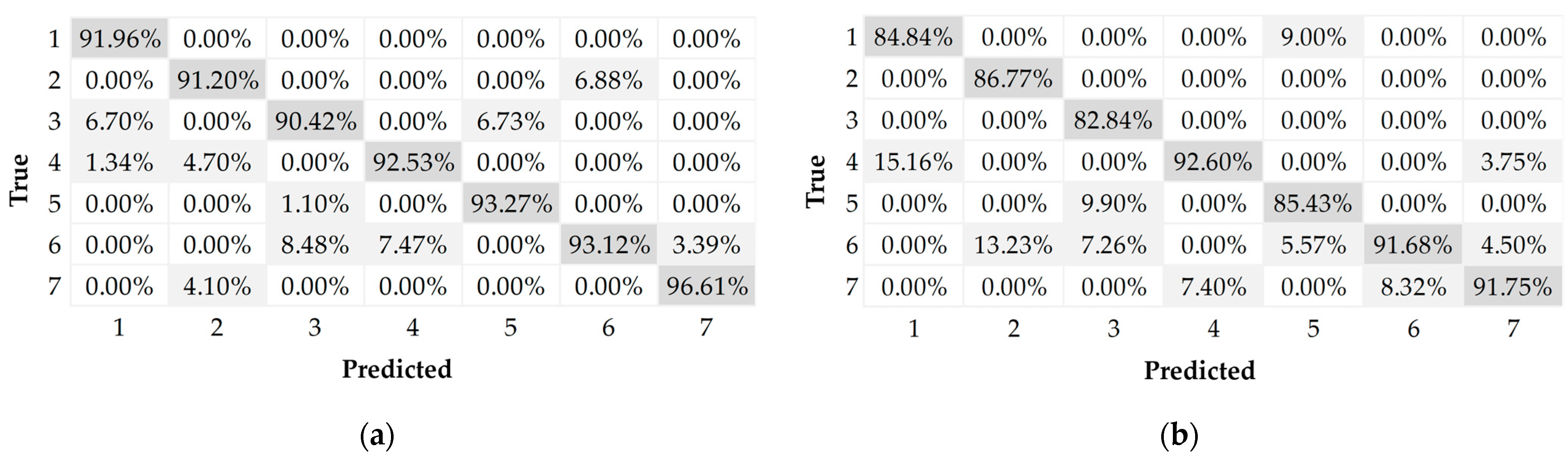
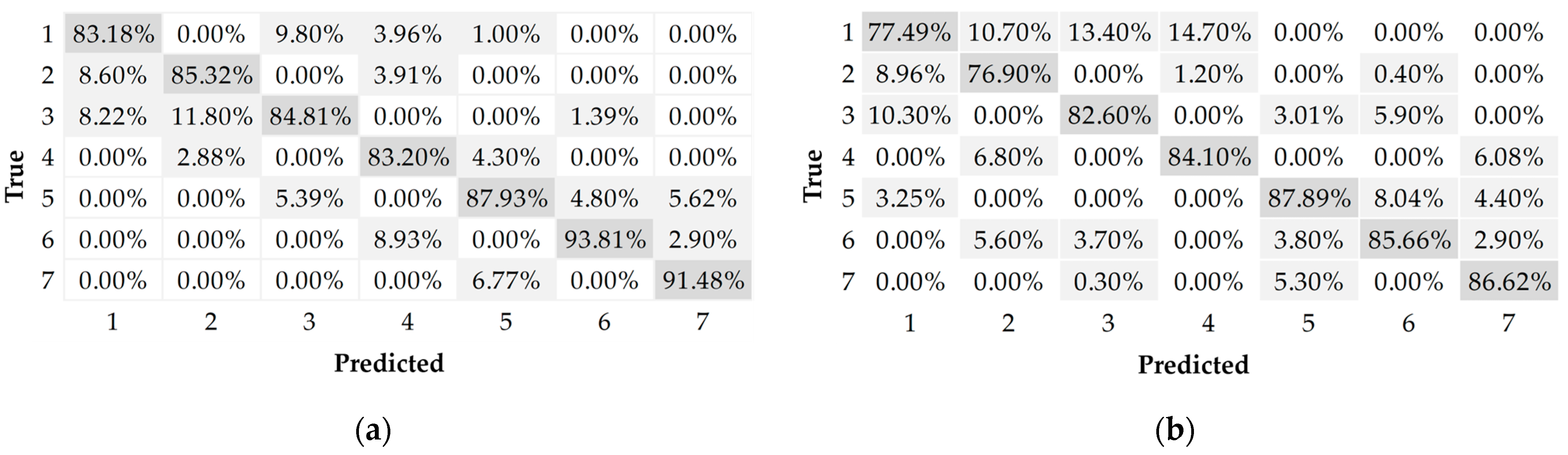
It is important to show graphically and analytically the performance of the artificial neural networks developed in synchrony with the control charts proposed to detect and interpret the source of variation. Therefore, ROC curves were developed; see Figure 7. Figure 8 and Figure 9 show the confusion matrices generated after validating the implementation of the multilayer perceptron ANN and SVM integrated with the MCUSUM and MEWMA control charts, respectively.
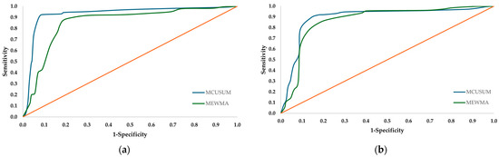
Figure 7.
ROC analysis validation phase. (a) Multilayer perceptron ANN; (b) SVM.
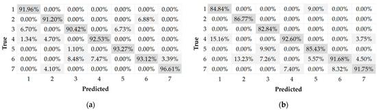
Figure 8.
Confusion matrix of the multilayer perceptron ANN. (a) MCUSUM control chart; (b) MEWMA control chart.
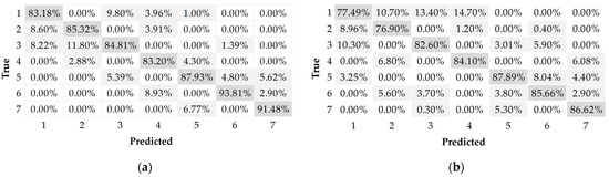
Figure 9.
Confusion matrix of the SVM. (a) MCUSUM control chart; (b) MEWMA control chart.
According to the results, the multilayer perceptron artificial neural network has a higher probability of correctly discriminating the source of variability occurring in the operation, both with the MCUSUM and MEWMA control chart, achieving a performance of 91.2% and 88.1%, respectively. The best classification result achieved with the SVM is from working together with the MCUSUM chart, reaching a probability of 87.3%. As for the confusion matrices, the success of the classification model is evaluated by comparing the predictions of the trained model against the real values; in this scheme, both multilayer perceptron ANN and SVM present a lower classification performance in the categories where variability associated with a single variable is present, which is predictable since a lower degree of variability in the operation is analyzed.
5. Discussion
Once the results were analyzed, the methodology is structured according to the efficiency for the statistical monitoring of the process by the control charts and the capacity of the artificial neural networks to classify and interpret the source variation generated in the process. Regarding the statistical monitoring phase of the process, the operation of the MCUSUM graph focuses on accumulating the variability of past measurements and does not depend on a memory weighting like the MEWMA graph, thus achieving greater efficiency in detecting special variability in the manufacturing operation. With respect to the variability classification and interpretation stage, it is important to highlight the ability of multilayer perceptron ANN to classify nonlinear relationships in the data, such as the variability structure in the processes. On the other hand, a disadvantage of using the SVM is that the number of models required increases as the number of classes of the analyzed problem increases.
The methodology is defined from the integration between the MCUSUM control chart and the multilayer perceptron ANN, allowing a strict and efficient surveillance of the critical quality characteristics monitored in the solder paste application operation by interpreting the variability with a sensitivity level of 92.41% and specificity of 91.16%. In this way, organizations will be able to define the source of variation in their processes in a reliable, expressive, and easy-to-interpret manner. The competitive advantage of the developed methodology is centered on being able to make pertinent adjustments to the manufacturing systems in a timely manner, guaranteeing process productivity, product quality, and customer satisfaction.
As future work, classification models such as probabilistic and convolutional neural networks will be implemented with the intention of comparing their efficiency in the classification of variability in manufacturing processes against the results shown.
Author Contributions
Conceptualization, E.A.R.-S., V.F.-F. and M.T.-E.; methodology, E.A.R.-S. and Y.V.P.-P.; validation, E.A.R.-S., E.B.-S. and J.C.-S.; formal analysis, E.A.R.-S. and J.C.-S.; investigation, E.A.R.-S., Y.V.P.-P., E.B.-S., V.F.-F. and M.T.-E.; writing—original draft preparation, E.A.R.-S.; writing—review and editing, E.A.R.-S. and Y.V.P.-P. All authors have read and agreed to the published version of the manuscript.
Funding
This research received no external funding.
Institutional Review Board Statement
Not applicable.
Informed Consent Statement
Not applicable.
Data Availability Statement
The original contributions presented in this study are included in the article; further inquiries can be directed to the corresponding author.
Conflicts of Interest
The authors declare no conflicts of interest.
References
- Li, L.; Xu, S.X.; Ning, Y.; Liu, Y.; Yang, S. How should companies deploy their digital supply chain platforms to gain competitive advantages? An asset orchestration perspective. Inf. Manag. J. 2023, 60, 103–842. [Google Scholar] [CrossRef]
- Bottani, E.; Montanari, R.; Volpi, A.; Tebaldi, L. Statistical process control of assembly lines in manufacturing. J. Ind. Inf. Integr. 2023, 32, 100435. [Google Scholar] [CrossRef]
- Wan, Q.; Zhu, M.; Qiao, H. A joint design of production, maintenance planning and quality control for continuous flow processes with multiple assignable causes. CIRP J. Msanuf. Sci. Technol. 2023, 43, 214–226. [Google Scholar] [CrossRef]
- Abubakar, A.S.; Hajej, Z.; Nyoungue, A.C. An optimal production, maintenance and quality problem, with improved statistical process chart of a supply chain under service and quality requirements. IFAC-PapersOnLine 2022, 55, 1746–1751. [Google Scholar] [CrossRef]
- Rasay, H.; Taghipour, S.; Sharifi, M. An integrated Maintenance and Statistical Process Control Model for a Deteriorating Production Process. Reliab. Eng. Syst. Saf. 2022, 228, 108–774. [Google Scholar] [CrossRef]
- De Almeida Moreira, B.R.; Cruz, V.H.; Cunha, M.L.O.; Da Silva Viana, R. Full-scale production of high-quality wood pellets assisted by multivariate statistical process control. Biomass Bioenergy 2021, 151, 106–159. [Google Scholar] [CrossRef]
- Shojaee, M.; Noori, S.; Jafarian-Namin, S.; Johannssen, A. Integration of production–maintenance planning and monitoring simple linear profiles via Hotelling’s T2 control chart and particle swarm optimization. Comput. Ind. Eng. 2023, 188, 109864. [Google Scholar] [CrossRef]
- Ueda, R.M.; Souza, A.M. An effective approach to detect the source(s) of out-of-control signals in productive processes by vector error correction (VEC) residual and Hotelling’s T2 decomposition techniques. Expert Syst. Appl. 2022, 187, 115–979. [Google Scholar] [CrossRef]
- Zaman, B.; Lee, M.H.; Riaz, M.; Abujiya, M.R. An improved process monitoring by mixed multivariate memory control charts: An application in wind turbine field. Comput. Ind. Eng. 2020, 142, 106–343. [Google Scholar] [CrossRef]
- Sikder, S.; Mukherjee, I.; Panja, S.C. A synergistic Mahalanobis–Taguchi system and support vector regression based predictive multivariate manufacturing process quality control approach. J. Manuf. Syst. 2020, 57, 323–337. [Google Scholar] [CrossRef]
- Ahsan, M.; Aulia, T.R. Comparing the Performance of Several Multivariate Control Charts Based on Residual of Multioutput Least Square SVR (MLS-SVR) Model in Monitoring Water Production Process. J. Phys. Conf. Ser. 2021, 2123, 012018. [Google Scholar] [CrossRef]
- Anojahatlo, K.; Sabri-Laghaie, K. Enhancing the detection power of multivariate time between events control charts for Gumbel’s bivariate exponential distribution. Comput. Ind. Eng. 2022, 171, 108–215. [Google Scholar] [CrossRef]
- Lee, P.; Torng, C.; Lin, C.; Chou, C. Control chart pattern recognition using spectral clustering technique and support vector machine under gamma distribution. Comput. Ind. Eng. 2022, 171, 108437. [Google Scholar] [CrossRef]
- Zaidi, F.S.; Dai, H.L.; Imran, M.; Tran, K. Analyzing abnormal pattern of hotellingT2control chart for compositional data using artificial neural networks. Comput. Ind. Eng. 2023, 180, 109–254. [Google Scholar] [CrossRef]
- Wang, K.; Asrini, L.J. Multivariate auto-correlated process control by a residual-based mixed CUSUM-EWMA model. Qual. Reliab. Eng. 2023, 39, 1120–1142. [Google Scholar] [CrossRef]
- Imran, M.; Dai, H.; Zaidi, F.S.; Hu, X.; Tran, K.P.; Sun, J. Analyzing out-of-control signals of T2 control chart for compositional data using artificial neural networks. Expert Syst. Appl. 2024, 238, 122–165. [Google Scholar] [CrossRef]
- Güler, Z.; Bakır, M.A.; Kardïyen, F. A novel hybrid ICA-SVM method for detection and identification of shift in multivariate processes. Hacet. J. Math. Stat. 2024, 53, 556–576. [Google Scholar] [CrossRef]
- Li, X.; Liu, G.; Sun, S.; Yi, W.; Li, B. Digital twin model-based smart assembly strategy design and precision evaluation for PCB kit-box build. J. Manuf. Syst. 2023, 71, 206–223. [Google Scholar] [CrossRef]
- Chen, Y.; Zhong, J.; Mumtaz, J.; Zhou, S.; Zhu, L. An improved spider monkey optimization algorithm for multi-objective planning and scheduling problems of PCB assembly line. Expert Syst. Appl. 2023, 229, 120600. [Google Scholar] [CrossRef]
- Ling, Q.; Isa, N.A.M.; Asaari, M.S.M. SDD-Net: Soldering defect detection network for printed circuit boards. Neurocomputing 2024, 610, 128575. [Google Scholar] [CrossRef]
- Mehmood, R.; Riaz, M.; Lee, M.H.; Ali, I.; Gharib, M. Exact computational methods for univariate and multivariate control charts under runs rules. Comput. Ind. Eng. 2022, 163, 107821. [Google Scholar] [CrossRef]
- Taji, J.; Farughi, H.; Rasay, H. Economic-statistical design of fully adaptive multivariate control charts under effects of multiple assignable causes. Comput. Ind. Eng. 2022, 173, 108676. [Google Scholar] [CrossRef]
- Sabahno, H.; Amiri, A.; Castagliola, P. A new adaptive control chart for the simultaneous monitoring of the mean and variability of multivariate normal processes. Comput. Ind. Eng. 2020, 151, 106524. [Google Scholar] [CrossRef]
- Yao, W.; Li, D.; Gao, L. Fault detection and diagnosis using tree-based ensemble learning methods and multivariate control charts for centrifugal chillers. J. Build. Eng. 2022, 51, 104–243. [Google Scholar] [CrossRef]
- Imran, M.; Sun, J.; Zaidi, F.S.; Abbas, Z.; Nazir, H.Z. Effect of Measurement Error on the Multivariate CUSUM Control Chart for compositional Data. Comput. Model. Eng. Sci. 2023, 136, 1207–1257. [Google Scholar] [CrossRef]
- Van Nguyen, T.T.; Heuchenne, C.; Tran, K.P. Anomaly Detection for Compositional Data using VSI MEWMA control chart. IFAC-PapersOnLine. 2022, 55, 1533–1538. [Google Scholar] [CrossRef]
- Deka, M.J.; Kalita, P.; Das, D.; Kamble, A.D.; Bora, B.J.; Sharma, P.; Medhi, B.J. An approach towards building robust neural networks models using multilayer perceptron through experimentation on different photovoltaic thermal systems. Energy Convers. Manag. 2023, 292, 117395. [Google Scholar] [CrossRef]
- Mystkowski, A.; Wolniakowski, A.; Idzkowski, A.; Ciężkowski, M.; Ostaszewski, M.; Kociszewski, R.; Kotowski, A.; Kulesza, Z.; Dobrzański, S.; Miastkowski, K. Measurement and diagnostic system for detecting and classifying faults in the rotary hay tedder using multilayer perceptron neural networks. Eng. Appl. Artif. Intell. 2024, 133, 108513. [Google Scholar] [CrossRef]
- Alfred, R.; Chinthamu, N.; Jayanthy, T.; Muniyandy, E.; Dhiman, T.K.; John, T.N. Implementation of advanced techniques in production and manufacturing sectors through support vector machine algorithm with embedded system. Meas. Sens. 2024, 33, 101119. [Google Scholar] [CrossRef]
- Ghiasi, R.; Khan, M.A.; Sorrentino, D.; Diaine, C.; Malekjafarian, A. An unsupervised anomaly detection framework for onboard monitoring of railway track geometrical defects using one-class support vector machine. Eng. Appl. Artif. Intell. 2024, 133, 108167. [Google Scholar] [CrossRef]
- Cai, J.; Xi, N. Site classification methodology using support vector machine: A study. Earthq. Res. Adv. 2024, 100294. [Google Scholar] [CrossRef]
- Christilda, A.J.; Manoharan, R. Enhanced hyperspectral image segmentation and classification using K-means clustering with connectedness theorem and swarm intelligent-BiLSTM. Comput. Electr. Eng. 2023, 110, 108–897. [Google Scholar] [CrossRef]


Disclaimer/Publisher’s Note: The statements, opinions and data contained in all publications are solely those of the individual author(s) and contributor(s) and not of MDPI and/or the editor(s). MDPI and/or the editor(s) disclaim responsibility for any injury to people or property resulting from any ideas, methods, instructions or products referred to in the content. |
© 2024 by the authors. Licensee MDPI, Basel, Switzerland. This article is an open access article distributed under the terms and conditions of the Creative Commons Attribution (CC BY) license (https://creativecommons.org/licenses/by/4.0/).