Systematic Analysis of Low-Precision Training in Deep Neural Networks: Factors Influencing Matrix Computations

Abstract

As Deep Neural Networks (DNNs) continue to increase in complexity, the computational demands of their training have become a significant bottleneck. Low-precision training has emerged as a crucial strategy, wherein full-precision values are quantized to lower precisions, reducing computational overhead while aiming to maintain model accuracy. While prior research has primarily focused on minimizing quantization noise and optimizing performance for specific models and tasks, a comprehensive understanding of the general principles governing low-precision computations across diverse DNN architectures has been lacking. In this paper, we address this gap by systematically analyzing the factors that influence low-precision matrix computations, which are fundamental to DNN training. We investigate three critical factors—accumulation in matrix calculations, the frequency of element usage, and the depth of matrices within the model—and their impact on low-precision training. Through controlled experiments on standard models, as well as customized experiments designed to isolate individual factors, we derive several key insights: layers with higher accumulation and matrices with lower usage frequencies demonstrate greater tolerance to low-precision noise, without significantly compromising the stability of model training. Additionally, while the depth of matrices influences the stability of matrix operations to some extent, it does not have a noticeable effect on the overall training outcomes. Our findings contribute to the development of generalizable principles for low-precision training, offering a systematic framework applicable across various DNN architectures. We provide empirical evidence supporting the strategic allocation of training bit-widths based on the analyzed factors, thereby enhancing the efficiency and effectiveness of DNN training in resource-constrained environments.

1. Introduction

The training of Deep Neural Networks (DNNs) is inherently computationally intensive, demanding substantial time and memory resources [1,2]. For instance, training a large language model with 175 billion parameters requires approximately 1000 A100 GPUs (80 GB) running continuously for 33 days, while autonomous driving systems need to process up to 1.5 TB of sensor data per hour. As the complexity of these models continues to grow, so too does the need for strategies that can mitigate the associated computational overhead without compromising the quality of the resulting models. This pursuit has driven the development of various techniques, among which quantization training stands out as a pivotal approach. This technique is particularly vital in enabling the deployment of sophisticated models on platforms with limited resources, such as mobile devices (with typically 4–8 GB RAM) and embedded systems [3,4,5]. Quantization involves transforming high-precision models into their low-precision counterparts, thereby facilitating faster computations, reducing memory footprint, and making DNNs more accessible for real-time applications and energy-efficient environments.

However, this transformation is not without its challenges. The inherent trade-off between precision and performance remains a significant concern, as the process of quantization inevitably introduces noise, which can degrade model accuracy if not carefully managed. This trade-off highlights the delicate balance that must be struck between reducing computational demands and maintaining the integrity of the model’s predictions. The challenge is further compounded by the diverse architectures and varying computational characteristics of different DNN models, which makes it difficult to develop a one-size-fits-all solution.

In recent years, considering the diverse computational characteristics across different DNN layers, mixed-precision training—which flexibly allocates different bit-widths to different layers based on low-precision training—has emerged as a promising research direction. Many studies treat the bit-width of each layer as a hyperparameter of the model and determine appropriate bit-widths through Quantization-Aware Training (QAT) [6,7]. However, this approach primarily focuses on obtaining reasonable mixed-precision inference models without optimizing the DNN training process. Common methods for optimizing DNN training typically require in-depth analysis of the training process and treat bit-width selection as an optimization problem [8,9,10], or employ specially tailored data formats and optimization strategies [11,12,13]. While these strategies enable more fine-grained trade-offs between computational resources and model accuracy, particularly suitable for energy-efficient scenarios, they often lack universality despite performing well on specific tasks. This makes them challenging to adapt to emerging models and architectures, or they require complex analysis processes with substantial optimization overhead and difficulty. With the rapid advancement of deep learning technology and increasing diversity and complexity of model architectures, there is an urgent need for mixed-precision training techniques that offer broad applicability and can quickly and efficiently adapt to different models.

To discover universally applicable mixed-precision training strategies across different DNN architectures, a systematic investigation of the patterns affecting low-precision training effectiveness is essential. Rather than greedily minimizing low-precision errors during training or pursuing optimization for specific tasks, our paper approaches the problem from the perspective of low-precision matrix computations in DNN training, analyzing how matrices with different characteristics affect computational results under low-precision quantization. By examining three key factors—the number of accumulations in matrix calculations, element usage frequency, and the depth of matrices within the model—we reveal how these factors influence model convergence and stability under various low-precision training configurations, and explore the underlying universal patterns. We design and implement a series of comparative experiments, including both typical DNN model experiments and customized experiments aimed at isolating individual factors. Through these experiments, the following key patterns emerge: First, layers with higher accumulation counts and matrices with lower usage frequencies demonstrate greater tolerance to low-precision quantization noise without significantly impacting model training effectiveness. Second, while matrix depth influences the stability of matrix operations to some extent, its impact on overall training results is relatively minimal. These universal patterns eliminate the need for detailed analysis and optimization of computational processes, facilitating efficient DNN training and deployment.

Our contributions in this work are twofold. First, we provide a systematic analysis of the impact of quantization noise on various computational factors within DNNs. This analysis offers a theoretical framework that can guide the implementation of low-precision training strategies across different models, ensuring that these strategies are both effective and adaptable. Second, we introduce a set of generalizable principles for low-precision training that can be readily applied to a wide range of DNN architectures. By addressing the need for a universally applicable and theoretically grounded approach to low-precision training, our work paves the way for more efficient and effective deep learning models that are capable of meeting the demands of modern applications while operating within the constraints of limited computational resources.

2. Related Work

2.1. Quantization

Quantization has emerged as a fundamental technique in deep learning, particularly for reducing model size and accelerating inference in resource-constrained environments [14]. This approach involves representing weights and activations with fewer bits, thereby compressing the model while striving to preserve its accuracy [15,16,17,18]. By reducing the precision of the numerical representations, quantization decreases both the memory footprint and the computational demand, making it possible to deploy sophisticated models on devices with limited computational resources, such as mobile phones and embedded systems.

The exploration of quantization techniques has led to the development of several innovative methods. Early approaches, such as binary and ternary weight networks [19,20], have shown that substantial model compression can be achieved with minimal performance degradation. These methods rely on the observation that high-precision weights often contain significant redundancy, which can be reduced without severely impacting the model’s ability to make accurate predictions.

Furthermore, research has expanded into various forms of quantization, such as uniform and non-uniform quantization [21,22]. Uniform quantization assigns equal spacing between quantization levels, making it straightforward to implement, while non-uniform quantization allows for more flexible and efficient use of bit-widths by adapting to the distribution of the model’s parameters. Techniques like mixed-precision quantization have also been developed, where different parts of the network are quantized to different levels of precision depending on their sensitivity to quantization noise. This not only helps in maintaining accuracy but also optimizes the computational efficiency of the model.

2.2. QAT

Quantization-Aware Training (QAT) represents a significant evolution in the application of quantization techniques within the training process of deep neural networks. Unlike post-training quantization, where the model is quantized after being fully trained, QAT integrates quantization into the training loop itself, allowing the model to learn how to cope with the reduced precision from the outset [3,10,23,24,25]. This approach ensures that the final model is better adapted to low-precision hardware, potentially leading to smaller and faster models that do not sacrifice accuracy [26].

The core idea behind QAT is to simulate the effects of quantization during training by quantizing the weights and activations in each forward pass while maintaining full precision during the backward pass [27]. This process allows the network to learn to be robust to the quantization process, effectively “pre-conditioning” it for deployment on low-precision hardware. The pioneering work demonstrated that by integrating quantization into the training process, models could be optimized for efficient integer arithmetic during inference, significantly reducing the computational overhead [4].

Recent advancements in QAT have focused on enhancing its flexibility and robustness. Techniques such as stochastic rounding have been introduced to mitigate the impact of quantization noise by randomly rounding the weights and activations, which helps in maintaining the gradient flow during training. Additionally, researchers have developed methods to adaptively adjust the quantization parameters, such as the bit-widths, during training based on the model’s performance [6,28]. This dynamic adjustment allows for a more fine-grained control over the trade-off between model size and accuracy, making QAT applicable to a wider range of models and tasks [29].

Moreover, QAT has been extended to support mixed-precision training, where different layers of the network are trained at different precision levels based on their sensitivity to quantization [30,31,32]. This approach allows for more efficient use of the available bit-widths, enabling the training of larger models on the same hardware [33].

2.3. FQT

Full Quantization Training (FQT) represents the next frontier in the evolution of quantization techniques, where not only the weights and activations but also the gradients are quantized during the training process [34,35,36,37,38,39,40,41]. This comprehensive approach to quantization aims to fully leverage the benefits of low precision throughout the entire training process, potentially leading to significant improvements in both training efficiency and model deployment [13].

The primary motivation behind FQT is to extend the benefits of low precision to the backward pass of training, where gradients are calculated and used to update the model’s weights. By quantizing gradients, FQT reduces the memory bandwidth and computational requirements of training, which can be particularly beneficial for large-scale models trained on distributed systems [42]. However, this approach also introduces additional challenges, particularly in terms of numerical stability, as low-precision gradients can lead to inaccuracies in the weight updates, potentially hindering the convergence of the model [8].

To address these challenges, FQT methods often employ a variety of techniques to stabilize the training process. For example, dynamic scaling of gradients is a common approach, where the gradients are scaled to a higher precision during critical stages of training to prevent numerical errors [43,44]. Additionally, gradient clipping is frequently used to limit the range of gradient values, reducing the risk of instability during training. These techniques are crucial for ensuring that FQT can achieve competitive performance while maintaining the efficiency benefits of low-precision training.

Recent research in FQT has also explored the use of mixed-precision training, where different parts of the network are trained with different levels of precision [9,45]. This approach allows for a more flexible and adaptive training process, where the precision can be adjusted based on the specific needs of each layer or operation within the network [46].

3. Low Precision in Matrix Calculations

The training process of DNNs relies on matrix computations. Prior work has predominantly focused on reducing low-precision noise during computations or adapting to low precision in training to optimize a set objective, without summarizing patterns specific to the operational characteristics of different matrices [47]. In this section, we focus our analysis on three factors: accumulations in Matrix Calculations (Section 3.1), frequency of elements in the matrix are used (Section 3.2), and depth of matrix in DNN (Section 3.3). Through experimentation as shown in Figure 1, we analyze the Euclidean distance between results and ground truth values under different factors, trying to uncover the underlying regularities.

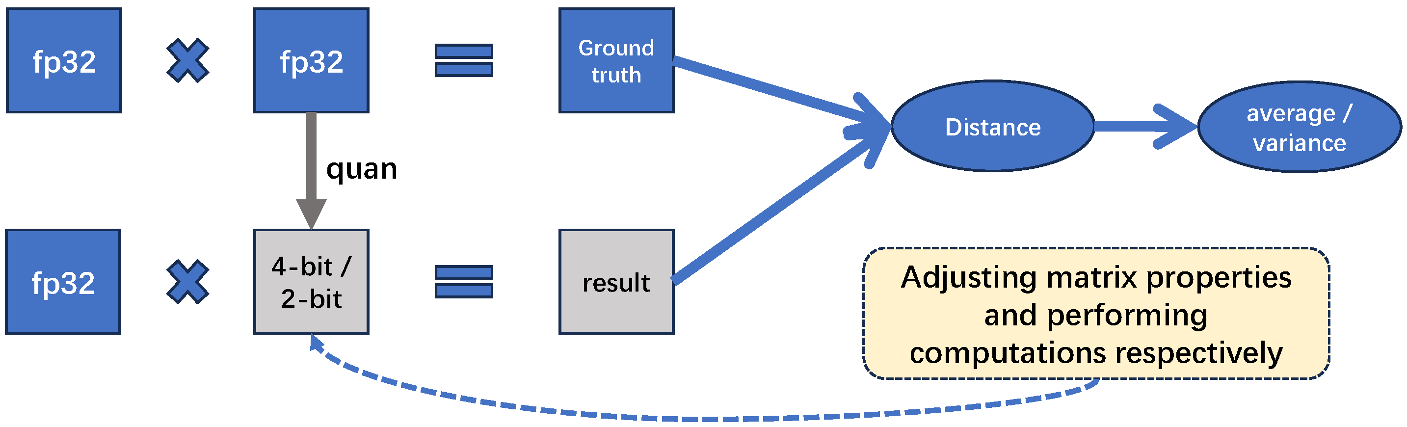
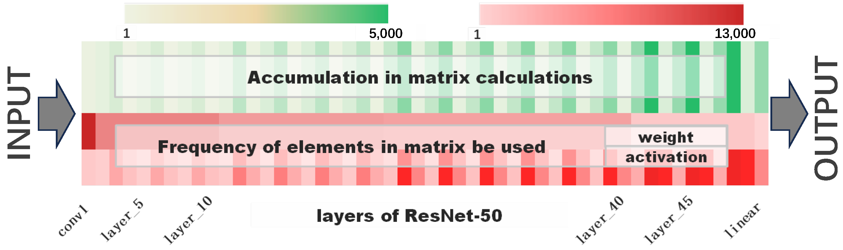
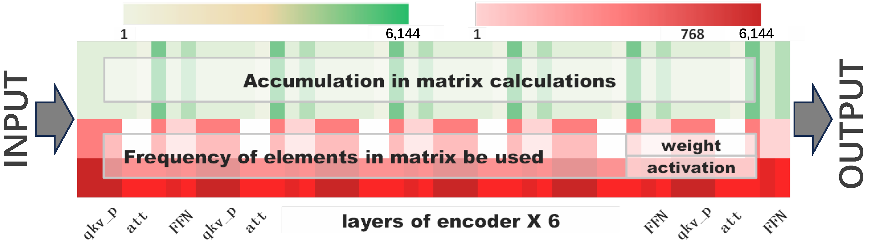
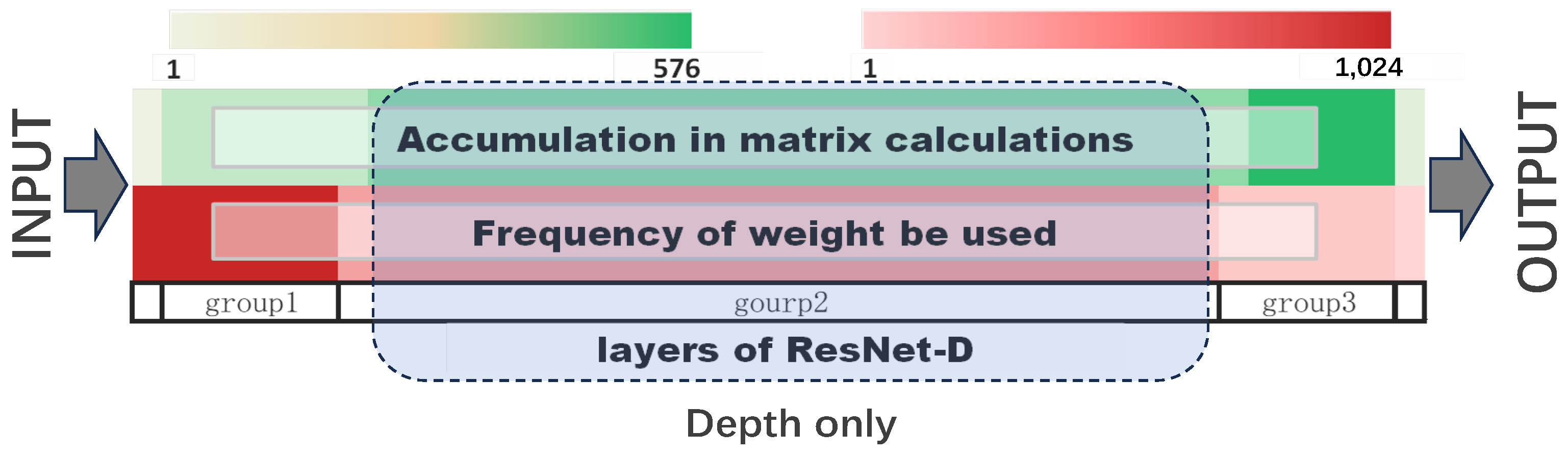
3.1. Accumulation in Matrix Calculations

For DNNs, the computations involved in the model are typically realized through matrix multiplications. Consider the multiplication of two matrices of real numbers, $r_1$ and $r_2$, with their product represented by $r_3=r_1{r}_2$ calculated in full precision (FP32). We denote the entries of each of these matrices $r_{\alpha }(\alpha =$ 1, 2 or 3) and the elements in it as $r_{\alpha }^{(i,j)}$. In the quantization calculation, quantization errors ${ϵ}_1$ and ${ϵ}_2$ are added to $r_1$ and $r_2$. At this time, the calculation of elements in $r_{q,3}$ can be written as

$$r_{q,3}^{(i,k)}=\sum _{j=1}^N(r_1^{(i,j)}+{ϵ}_1^{(i,j)})(r_2^{(j,k)}+{ϵ}_2^{(j,k)})$$

(1)

which can be rewritten as

$$\begin{array}{c}\hfill r_{q,3}^{(i,k)}=\sum _{j=1}^N{r}_1^{(i,j)}{r}_2^{(j,k)}+\sum _{j=1}^N{r}_1^{(i,j)}{ϵ}_2^{(j,k)}+\sum _{j=1}^N{ϵ}_1^{(i,j)}{r}_2^{(j,k)}+\sum _{j=1}^N{ϵ}_1^{(i,j)}{ϵ}_2^{(j,k)}\end{array}$$

(2)

The first term in the Formula (2) is equal to the value calculated in full precision, and the last three terms are errors caused by low-precision quantization. A direct idea is to reduce the impact of the last three items on the calculation as much as possible.

Let us take the term ${\sum }_{j=1}^N{r}_1^{(i,j)}{ϵ}_2^{(j,k)}$ as an example. Since $r_1$ is a matrix and ${ϵ}_2$ represents the noise of another matrix, they are mutually independent. Therefore, $E\left(r_1{ϵ}_2\right)=E\left(r_1\right)·E\left({ϵ}_2\right)$. In the training of DNNs, low-precision quantization errors can be regarded as random errors with a mathematical expectation of zero, i.e., $E\left({ϵ}_2\right)=0$. Consequently, the mathematical expectation of ${\sum }_{j=1}^N{r}_1^{(i,j)}{ϵ}_2^{(j,k)}$, denoted as $E\left[{\sum }_{j=1}^N{r}_1^{(i,j)}{ϵ}_2^{(j,k)}\right]$, equals 0. However, when the sample size is relatively small, the sample values may not necessarily converge to their mathematical expectation. Thus, only when N is sufficiently large can this term approach 0. The same principle applies to ${\sum }_{j=1}^N{ϵ}_1^{(i,j)}{r}_2^{(j,k)}$ and ${\sum }_{j=1}^N{ϵ}_1^{(i,j)}{ϵ}_2^{(j,k)}$.

In DNN training, various matrices of different size are required to perform multiplication operations. Figure 2 and  Figure 3 illustrate the accumulation count of elements involved in computations across different layers for models based on ResNet-50 and Transformer, respectively. It is evident that in DNN computations, there is a significant disparity in the number of elements participating in calculations along the model, suggesting that the tolerance for low-precision noise also varies considerably.

We employ 50 random experiments for our observations: As shown in Figure 1, initially, we perform matrix multiplication using full precision, and we consider the outcome as the ground truth. Subsequently, we quantize one of the matrices to low precision (i.e., 4-bit and 2-bit) and carry out the same multiplication operation, recording the average distance of each element in the computed result from its corresponding element in the ground truth. To examine the impact of the accumulation count of elements involved in the computation, we alter the matrix size to progressively increase the number of elements (from 9 to 2304, from the same distribution) participating in the matrix calculation, and sequentially document the distance between the computed results and their ground truth at this time.

Figure 4 illustrates that regardless of the bit-width (4-bit or 2-bit), the distance introduced by low precision consistently decreases as the number of elements increases. More importantly, the variance of the distance significantly improves, indicating a more stable computation, which is highly beneficial for the convergence of DNN training.

3.2. Frequency of Elements in the Matrix Used

When calculating $r_3=r_1{r}_2$, the elements of $r_3$ are obtained by multiplying the rows of matrix $r_1$ with the columns of matrix $r_2$ and then summing the results. In the process of computing $r_3$, it is noted that the elements in matrices $r_1$ and $r_2$ are utilized with different frequencies, which is related to the dimensions of the matrices being multiplied, e.g., when the number of columns in $r_2$ is less than the number of rows in $r_1$, matrix $r_2$ is accessed more frequently.

For the convenience of analysis, we assume that matrix $r_1$ is an $M\times N$ matrix, and $r_2$ is an $N\times 1$ matrix. In this case, the elements obtained from the low-precision matrix multiplication $r_3$ in Equation (2) can be represented as

$$\begin{array}{c}\hfill r_{q,3}^{(i,1)}=\sum _{j=1}^N{r}_1^{(i,j)}{r}_2^{(j,1)}+\sum _{j=1}^N{r}_1^{(i,j)}{ϵ}_2^{(j,1)}+\sum _{j=1}^N{ϵ}_1^{(i,j)}{r}_2^{(j,1)}+\sum _{j=1}^N{ϵ}_1^{(i,j)}{ϵ}_2^{(j,1)}\end{array}$$

(3)

In Equation (3), it is evident that the quantization noise from the two matrices has distinct impacts: the quantization noise in $r_2^{(i,1)}$ affects all elements in $r_3$ (for any i), while the quantization noise in $r_1^{(i,j)}$ only influences the i-th row of elements in $r_3$.

We adopt a methodology similar to that described in Section 3.1. In our matrix multiplication operations (Figure 1), we incrementally increase the size of one matrix (from the same distribution) to reduce the usage frequency of each element within the multiplication (from 512 to 9). We utilize the results computed in full precision as the ground truth and compare the average distance of each element between the low-precision computation results and the ground truth under different usage frequencies. Additionally, we analyze the fluctuation of these distances across multiple experiments.

As shown in Figure 5, the graph demonstrates the impact of quantization as matrix usage frequency decreases. For both 4-bit and 2-bit quantization, while the distance metrics (solid lines) remain relatively stable, there are notable differences in their absolute values, with 2-bit quantization showing consistently higher distances. This indicates a greater loss in precision with lower-bit quantization. The most striking observation is the significant downward trend in variance (dashed lines) as frequency decreases. This trend is particularly pronounced in the logarithmic scale of variance, suggesting that matrices with lower usage frequencies exhibit better tolerance to quantization noise. This enhanced tolerance contributes positively to the numerical stability during model training, making these matrices more suitable candidates for aggressive quantization strategies.

In DNN computations, due to the significant difference in the usage frequency of different matrices (as depicted in Figure 2 and  Figure 3), the impact of quantization on each matrix also varies. Matrices that are frequently used have a more extensive error impact. Consequently, the quantization errors are amplified with the increased usage of these matrices.

3.3. Depth of Matrix in DNN

In DNNs, layers situated at varying depths are tasked with unique functions. Shallow layers are typically charged with the initial extraction of rudimentary features from input data, such as discerning edges and textures [48]. In contrast, deeper layers delve into the extraction of more sophisticated and abstract features [49,50,51,52]. Furthermore, the sequential, layer-wise computation inherent in both the forward and backward propagations of DNNs means that quantization noise emerging from one layer has the potential to propagate, thereby influencing subsequent computational steps [8,10]. Building on this understanding, we posit that the depth at which low-precision matrix computations are performed could similarly impart diverse effects on the training process.

We also employ 50 independent experiments for observation (Figure 1). We set up three matrices of identical dimensions and perform matrix multiplication with the input sequentially, using the results as the ground truth. Subsequently, we apply low-precision quantization to each of these matrices and observe the impact of quantizing different matrices under the same quantization scheme on the final results. We then analyze the distance from the ground truth and the variance of this distance.

As shown in Figure 6, the graph illustrates the effects of quantization across different network depths. The distance metrics for both 4-bit and 2-bit quantization maintain relatively consistent values as depth increases, with 2-bit quantization consistently showing higher distance values. This stability in distance metrics suggests a certain “self-correction” capability within deeper networks. The variance exhibits a gradual declining trend with increasing depth, with higher variance observed in shallower layers. This observation is particularly significant as it indicates that quantization in shallow layers has a more substantial impact on computational stability compared to deeper layers. This finding has important implications for quantization strategy design, suggesting that more precise quantization approaches should be applied to shallow network layers to ensure overall computational stability.

4. Experimental Results on DNNs

In Section 3, we analyze the impact of the three factors on computation through simple matrix multiplication. However, DNNs are complex, interrelated networks, making it necessary to examine the influence of these factors on mixed-precision training within actual DNN models.

In this section, we empirically validate the impact of the three factors on the training bit-width utilized by layers: (a) accumulation in matrix calculations, (b) frequency of elements in matrix utilization, and (c) depth of matrix within DNNs. We initially present our experimental setup in Section 4.1, with a focus on the methodology of comparative experiments. Subsequently, in Section 4.2, we exhibit comprehensive experimental results on commonly used models. And in Section 4.3, we design customized models that separate the three factors to observe the impact on training.

4.1. Experimental Setup

Models and datasets. We train the AlexNet network [53], ResNet [54], and MobileNet-V2 [55] on the CIFAR-10/100 [56] and the ImageNet [57]. Additionally, for language modeling tasks, we train the Transformer model [58] on the WikiText-103 [59] and the LSTM model [60] on the PTB [61].

Training settings. We utilize the standard training setting in all our experiments, including epoch, batch size, momentum, learning rate, and other hyperparameters. Specifically, we follow SOTA settings in [62] for CIFAR-10 and [54] for ImageNet. We follow [63] for Transformer on WikiText-103 and [64] for LSTM on PTB. We opt to implement the GMMLOWP quantization scheme, which is extensively documented in Google’s open-source repository [4]. Our experiments are based on the classic low-precision training framework presented in [34], which has demonstrated comparable performance to full precision across various models and tasks using uniform low-precision. For instance, when training ResNet-50 on ImageNet, the accuracy degradation is less than 1% compared to its full precision counterpart. Our code adjusts the bit width based on the open-source repositories [34] and CPT method [46]. To mitigate the influence of stochastic elements in our experiments, the results are averaged over four runs.

Precision settings. In our experiments, we investigate the impact of weight quantization on training. We compress the weights of different layers to various bit-widths and train the models to observe the final training performance. Referring to Section 3, we establish three comparative factors:

• A: The training bit-width is set based on the number of Accumulations in matrix multiplication during computation.
• F: The training bit-width is set based on the Frequency with which elements in the matrix are used during computation.
• D: The training bit-width is set based on the Depth of the matrix within the model.

Concurrently, we establish the following four strategies for bit-widths of layers:

• U: Regardless of the variations in the comparative factors, assign the same training bit-width to all layers (the method proposed in [34]).
• C+: Set the training bit-width according to the comparative factors, with a positive correlation to the comparative factors.
• C−: Set the training bit-width according to the comparative factors, with a negative correlation to the comparative factors.
• R: Randomly assign training bit-widths to each layer.

Since higher bit-widths typically provide more accurate numerical representations while simultaneously increasing model size, we conduct comparative experiments using similar bit-width ranges and model sizes to ensure fair comparisons between different strategies.

4.2. Performance on Commonly Used Models

We conduct comparative experiments, focusing on three factors and training DNNs using four different training strategies based on each factor, recording the final model’s test accuracy/perplexity.

Table 1. Final training performance corresponding to bit-width strategies set according to the different factors. For instance, the value 85.51 in the second row and fifth column indicates that, with a positive correlation between the number of accumulations in matrix calculations and the computational bit-width (where higher accumulation counts in matrix operations correspond to a higher bit-width), the resulting test accuracy is 85.51 (‘Acc-A/Acc-F/Acc-D’ denotes the controlled factor is Accumulation in matrix calculations/Frequency of elements in matrix be used/Depth of Matrix in DNN). $\alpha$ is the width multiplier defined in [65].

Model	Dataset	#Bit	Strategy	Acc-A	Acc-F	Acc-D
AlexNet	CIFAR-10	6	U	85.46	85.46	85.46
AlexNet	CIFAR-10	4 to 8	C+	85.51	85.88	85.27
AlexNet	CIFAR-10	4 to 8	C−	86.00	85.27	85.88
ResNet-20	CIFAR-10	6	U	91.51	91.51	91.51
ResNet-20	CIFAR-10	4 to 8	C+	91.09	91.57	91.02
ResNet-20	CIFAR-10	4 to 8	C−	91.64	91.02	91.57
ResNet-20	CIFAR-100	6	U	68.40	68.40	68.40
ResNet-20	CIFAR-100	4 to 8	C+	68.37	68.60	68.33
ResNet-20	CIFAR-100	4 to 8	C−	68.71	68.33	68.60
ResNet-50	ImageNet	6	U	76.30	76.30	76.30
ResNet-50	ImageNet	4 to 8	C+	75.92	76.45	76.11
ResNet-50	ImageNet	4 to 8	C−	76.56	76.11	76.45
MobileNet-V2	ImageNet	6	U	66.45	66.45	66.45
MobileNet-V2	ImageNet	4 to 8	C+	65.19	66.67	64.31
MobileNet-V2	ImageNet	4 to 8	C−	66.79	64.31	66.67
MobileNet-V2 ($\alpha =0.5$)	ImageNet	6	U	55.61	55.61	55.61
MobileNet-V2 ($\alpha =0.5$)	ImageNet	4 to 8	C+	53.47	55.67	53.06
MobileNet-V2 ($\alpha =0.5$)	ImageNet	4 to 8	C−	55.85	52.13	55.67
Transformer	WikiText-103	7	U	32.30	32.30	33.09
Transformer	WikiText-103	6 to 8	C+	33.89	31.57	32.53
Transformer	WikiText-103	6 to 8	C−	31.60	33.55	31.30
2-LSTM	PTB	7	U	97.98	97.98	97.98
2-LSTM	PTB	6 to 8	C+	98.46	97.84	97.91
2-LSTM	PTB	6 to 8	C−	97.21	97.88	98.00

presents our experimental results, from which the following can be observed:

(1) There is a strong correlation between the accumulation in matrix computations and the capability to withstand quantization noise. Layers with a higher number of accumulations consistently achieved the best test performance when employing a lower training bit-width. This finding validates the analysis from Section 3.1, which suggests that layers with a larger number of accumulations can tolerate greater quantization noise, meaning they can effectively use lower training bit-widths, whereas layers with fewer accumulations require higher training bit-widths. Furthermore, in the case of MobileNet-V2, when the network width is reduced to half of its original size, the impact of correlation becomes more pronounced. As MobileNet-V2 is inherently a parameter-efficient model, it engages a relatively small number of parameters in computation. Once the model is narrowed, this leads to a further reduction in the aggregate quantity of parameters, consequently resulting in a significant decrease in accuracy. Additionally, the model becomes more sensitive to the effects of correlation.

(2) The frequency of elements in a matrix are used also correlates with the ability to resist quantization noise. Identical levels of quantization noise added to layers with lower usage frequencies often lead to superior training results. Even when optimal outcomes are not achieved for some tasks, the performance is still significantly better than with the opposite bit-width configuration strategy. This corroborates the analysis from Section 3.2, indicating that quantization noise in layers with higher usage frequencies has a more detrimental effect on training.

(3) In the context of CNN models, a decrement in the training bit-width at each layer with increasing depth yields improved outcomes. In contrast, for Transformer and LSTM models, such a trend is not evidently correlated. However, for CNN models, the trends in depth and usage frequency are same (as shown in Figure 2), resulting in completely consistent final outcomes, indicating a need for further analysis.

Reducing model size is also a significant benefit of low-precision quantization.

Table 2. Model size (MBit) corresponding to bit-width strategies set according to the different factors. For instance, the value 216 in the third row and fifth column indicates that, with a positive correlation between the number of accumulations in matrix calculations and the computational bit-width (where higher accumulation counts in matrix operations correspond to a higher bit-width), the size of the quantized model is 216 MBit (‘Size-A/Size-F/Size-D’ denotes the controlled factor is Accumulation in matrix calculations/Frequency of elements in matrix be used/Depth of Matrix in DNN).

Model	Dataset	#Bit	Strategy	Size-A	Size-F	Size-D
ResNet-20	CIFAR-10/100	6	U	1.12	1.12	1.12
ResNet-20	CIFAR-10/100	4 to 8	C+	1.08	1.05	1.20
ResNet-20	CIFAR-10/100	4 to 8	C−	1.01	1.20	1.05
ResNet-50	ImageNet	6	U	176	176	176
ResNet-50	ImageNet	4 to 8	C+	216	129	222
ResNet-50	ImageNet	4 to 8	C−	140	222	129
Transformer	WikiText-103	7	U	991	991	991
Transformer	WikiText-103	6 to 8	C+	977	1076	963
Transformer	WikiText-103	6 to 8	C−	1005	906	1019

lists the sizes of some experimental models from Table 1. It can be observed from Table 2 that for CNN models (ResNet-20/ResNet-50 on CIFAR-10/ImageNet), higher test accuracy does not require an increased model size. In fact, an appropriate bit-width allocation strategy can achieve greater accuracy with a reduced model size. In the case of the Transformer model, the sizes of the models with different bit-width allocation strategies do not differ significantly; however, a well-considered allocation strategy can lead to improved accuracy. Combining the observations from Table 1 and  Table 2, it is clear that different bit-width settings have a discernible impact on training. A judicious configuration strategy can effectively balance the reduction of model size while maintaining high accuracy.

Figure 7 shows the test accuracy and variance of different strategies using ResNet-20 on CIFAR-10/100 and ResNet-50 on ImageNet from 10 replicates. It can be seen that strategies that are negatively correlated with accumulation and positively correlated with frequency perform significantly more stably (smaller variance, represented by the area of circles) while achieving higher accuracy.

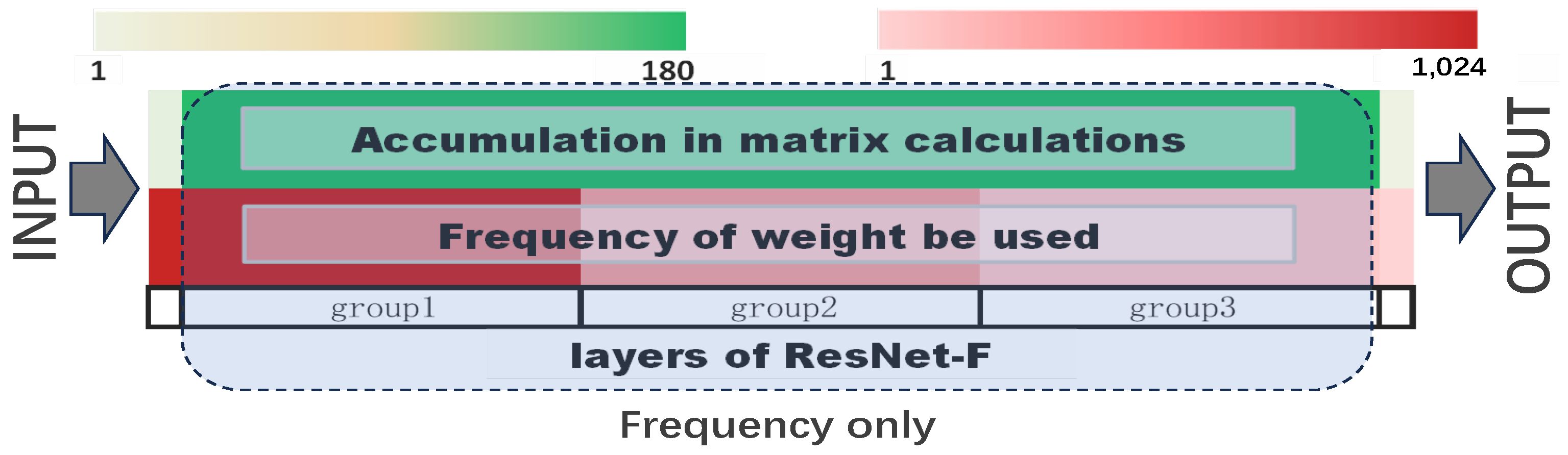
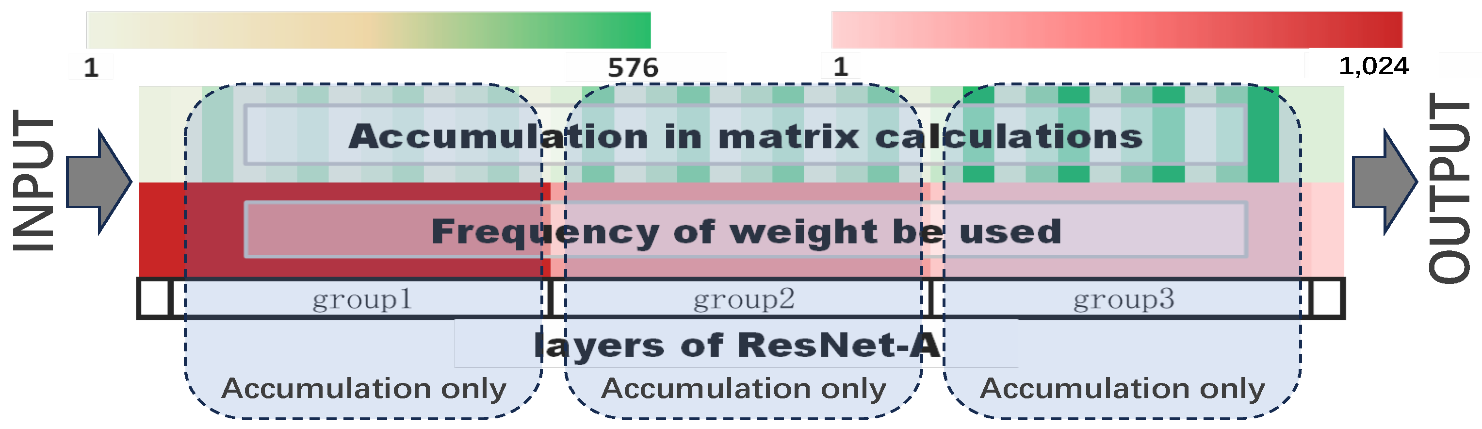
4.3. In-Depth Evaluation on Customized Models

Section 4.2 demonstrates experimental validation using common DNN models, reflecting the impact of three key factors on DNN mixed-precision training. However, due to the structural characteristics of these models, the three factors are not mutually independent (for instance, in CNN models, usage frequency and depth change in tandem), which hinders the separate analysis of each factor’s influence. Therefore, we conduct further evaluations and tailor models to achieve precise control over each factor, enabling a more detailed examination. Furthermore, we select different bit-width ranges to more comprehensively validate the training outcomes under various precision levels.

Factor of depth of matrix only. We modify the architecture of ResNet-20 on CIFAR: the original ResNet-20 consists of 18 layers divided into three groups, with each group containing three BasicBlocks, excluding the first conv layer and the last linear layer. Except for the first conv layer in each group, the BasicBlocks within the same group are composed of identical conv layers and have feature maps of the same size, meaning that the matrix operations in this part have the same number of accumulations and usage frequency. To investigate the impact of depth on DNN mixed-precision training, we expanded the second group to include 15 BasicBlocks. The model now comprises 44 layers, with 28 layers having the same number of accumulations and usage frequency (as shown in the dashed part of Figure 8), differing only in depth. For this part of the model, we can analyze the effect of depth on mixed-precision training independently. We denote this modified model as ResNet-D.

Table 3. Training ResNet-D on CIFAR-10: Test accuracy and variance based on depth-configured layer bit-Widths.

#Bit	Strategy	Acc-D	Variance
4 to 8	R	92.63	0.20
6	U	92.62	0.34
4 to 8	C+	92.83	0.31
4 to 8	C−	92.73	0.17
8 to 16	R	92.82	0.22
12	U	92.94	0.22
8 to 16	C+	92.92	0.23
8 to 16	C−	92.87	0.19

demonstrates that when depth serves as the only variable (with the number of accumulations in matrix calculations and usage frequency being consistent), there is no discernible correlation between the training bit-widths applied at each layer and the performance of the resulting model. Concurrently, Table 1 illustrates that for models like Transformer and LSTM, where depth and frequency do not change in tandem, the appropriate training bit-width does not exhibit a clear correlation when depth is the sole dominant factor. This indicates that the negative correlation between the appropriate training bit-width and depth observed in the CNN model of Table 1 is likely due more to differences in usage frequency or other factors rather than the depth itself. Additionally, it is observed that although the training bit-width strategy exhibiting a negative correlation with depth does not yield superior final performance, the stability of training is marginally better compared to other strategies. This finding aligns with the analysis presented in Section 3.3.

Factor of usage frequency only. From the analysis presented, it is evident that there is no significant correlation between the depth of layers and the suitable training bit-width. This observation raises the question of whether the matrix usage frequency is the primary factor that dictates the resilience against low-precision noise. However, since there is a certain correlation between usage frequency and the accumulation in matrix calculations (as shown in Figure 2 and Figure 3), it cannot be directly analyzed through commonly used models.

Therefore, to isolate the impact of usage frequency on the training bit-width at each layer during mixed-precision training, we modify the channel count of each group in the ResNet model to be uniform (with the thickness of the conv layers also being uniform), yet we still reduce the feature map at the first layer of each group. By ensuring that the accumulation in matrix calculation remains the same, we alter only the usage frequency to observe its effect on the training bit-width during mixed-precision training, as depicted in Figure 9. We denote this modified model as ResNet-F.

Table 4. Training ResNet-F on CIFAR-10: Test accuracy and variance based on frequency-configured layer bit-Widths.

#Bit	Strategy	Acc-F	Variance
4 to 8	R	90.56	0.41
6	U	90.88	0.32
4 to 8	C+	90.71	0.41
4 to 8	C−	90.54	0.60
8 to 16	R	91.77	0.36
12	U	92.02	0.33
8 to 16	C+	91.99	0.31
8 to 16	C−	91.79	0.60

reveals several crucial insights about the relationship between matrix usage frequency and quantization strategies during model training. Our analysis demonstrates that when maintaining fixed accumulation in matrix calculations while varying usage frequencies, Strategy U (which employs constant training bit-width) consistently outperforms other approaches. This superior performance can be attributed to its ability to maintain consistent numerical precision throughout the training process. A particularly noteworthy observation from our experiments is the strong correlation between model performance and matrix usage frequency [66,67]. Matrices with higher usage frequencies demonstrate heightened sensitivity to low-precision noise, as evidenced by both the performance metrics and variance measurements. This finding aligns with recent studies in Transformer model quantization [68,69], where activation quantization has proven to be particularly challenging. The correlation between usage frequency and quantization sensitivity is further substantiated by Figure 3, which illustrates the exceptionally high usage frequency of activations within Transformer architectures. This high frequency of use makes these matrices particularly susceptible to quantization effects, explaining why activation quantization often presents a significant challenge in practice. These findings lead to an important conclusion: matrices with high usage frequency during DNN training play a pivotal role in maintaining training stability. Their increased vulnerability to low-precision noise suggests that special attention should be paid to these matrices when designing quantization strategies. This understanding has significant implications for developing more effective quantization approaches, particularly in the context of large-scale Transformer models.

Factor of accumulations in matrix calculations only. We next analyze the impact of accumulation in matrix calculation separately. We build ResNet-A, a model that utilizes the BottleNeck structure. Within the same group, layers maintain uniform usage frequency and include both $3\times 3$ conv and $1\times 1$ conv, which have different accumulation counts in their computations, as shown in Figure 10. We set the training bit-widths according to the accumulation in matrix calculation and observe the experimental results.

Table 5. Training ResNet-A on CIFAR-10: Test accuracy and variance based on accumulation-configured layer bit-Widths.

#Bit	Strategy	Acc-A	Variance
6	U	86.61	2.37
4 to 8	C+	83.47	5.30
4 to 8	C−	86.67	1.49
7	U	92.32	0.39
6 to 8	C+	90.30	4.37
6 to 8	C−	92.41	0.29
12	U	92.81	0.23
8 to 16	C+	92.44	0.34
8 to 16	C−	92.85	0.23

reveals that strategy C− achieves the highest accuracy while significantly enhancing the stability of training. Concurrently, appropriately increasing the training bit-width for operations with fewer accumulation counts can substantially improve the final test accuracy (when the minimum bit-width is increased from 4 to 6, strategy C+ demonstrates notable improvement). This indicates that operations with fewer accumulation in matrix calculations are sensitive to low-precision noise and require efforts to minimize such noise. Therefore, layers with a higher number of accumulations in matrix computations possess better resilience against quantization noise and can utilize relatively lower training bit-widths.

5. Conclusions and Future Directions

In addressing the challenge of selecting optimal training bit-widths for layers within deep neural networks (DNNs), we have conducted a thorough investigation into the underlying patterns and characteristics inherent in DNN computations. Our analysis encompassed a detailed examination of matrix operations with varying features and comparative experiments across different DNN architectures. By isolating and studying individual factors through the use of customized models across a range of precision levels, we have derived several key conclusions:

1. Impact of Accumulations in Matrix Operations: The number of accumulations within matrix operations plays a crucial role in determining the accuracy and stability of low-precision computations. Specifically, during DNN training, layers characterized by a higher number of accumulations demonstrate a greater tolerance to the noise introduced by low-precision quantization. This suggests that such layers can operate effectively under reduced precision without compromising the overall integrity of the model.

2. Effect of Element Utilization Frequency: The frequency with which elements within matrix operations are utilized has a significant impact on the stability of low-precision computations. In the context of DNN training, matrices that experience high utilization frequencies necessitate the use of sufficiently high bit-widths to maintain the effectiveness and robustness of the training process. This finding underscores the importance of carefully considering element utilization when selecting bit-widths for different layers.

3. Influence of Matrix Depth: The position or depth of a matrix within the network architecture also affects low-precision matrix operations. However, our analysis indicates that in the context of DNN training, there is no consistent or clear correlation between the depth of low-precision matrices and the final performance of the trained model. This suggests that while matrix depth may influence certain aspects of computational behavior, it does not directly determine the success of low-precision training outcomes.

Several promising research directions emerge from our findings, warranting further exploration:

1. Bit-Width Selection in Large-Scale Language Models: The rapid evolution of large-scale language models [70] has popularized the pre-training and fine-tuning paradigm [71]. Future research should focus on analyzing the relationship between the bit-width used during training within this paradigm and the ultimate performance of the model. Identifying any underlying patterns could provide valuable insights for optimizing low-precision training in these increasingly prevalent models.

2. Adaptation to Emerging Model Architectures: The introduction of novel model architectures, such as Diffusion models [72] and Mixture of Experts (MOE) models [73], necessitates the investigation of how lower training bit-widths can be effectively applied within these frameworks. Furthermore, the development of new data formats [74] and quantization methods [75,76] presents additional challenges and opportunities for low-precision training, which merit comprehensive examination.

3. Theoretical Advancements in Low-Precision Training: Theoretical exploration of low-precision training remains a critical area of inquiry. Given the many unresolved questions in the field of DNNs, there is a compelling need to deepen our understanding of how bit-width impacts the data used during training. Such theoretical advancements could potentially unlock new strategies for enhancing the efficiency and effectiveness of DNN training, contributing to the broader goal of developing more robust and resource-efficient models.

References

1. Gholami, A.; Yao, Z.; Kim, S.; Hooper, C.; Mahoney, M.W.; Keutzer, K. Ai and memory wall. arXiv 2024, arXiv:2403.14123. [Google Scholar] [CrossRef]
2. Lewis, M.; Bhosale, S.; Dettmers, T.; Goyal, N.; Zettlemoyer, L. Base layers: Simplifying training of large, sparse models. In Proceedings of the International Conference on Machine Learning, PMLR, Virtual, 18–24 July 2021; pp. 6265–6274. [Google Scholar]
3. Courbariaux, M.; Bengio, Y.; David, J.P. Binaryconnect: Training deep neural networks with binary weights during propagations. In Advances in Neural Information Processing Systems; Curran Associates, Inc.: Red Hook, NY, USA, 2015; Volume 28. [Google Scholar]
4. Jacob, B.; Kligys, S.; Chen, B.; Zhu, M.; Tang, M.; Howard, A.; Adam, H.; Kalenichenko, D. Quantization and training of neural networks for efficient integer-arithmetic-only inference. In Proceedings of the IEEE Conference on Computer Vision and Pattern Recognition, Salt Lake City, UT, USA, 18–23 June 2018; pp. 2704–2713. [Google Scholar]
5. Lin, X.; Zhao, C.; Pan, W. Towards accurate binary convolutional neural network. In Advances in Neural Information Processing Systems; Curran Associates, Inc.: Red Hook, NY, USA, 2017; Volume 30. [Google Scholar]
6. Yang, H.; Duan, L.; Chen, Y.; Li, H. BSQ: Exploring bit-level sparsity for mixed-precision neural network quantization. arXiv 2021, arXiv:2102.10462. [Google Scholar]
7. Van Baalen, M.; Louizos, C.; Nagel, M.; Amjad, R.A.; Wang, Y.; Blankevoort, T.; Welling, M. Bayesian bits: Unifying quantization and pruning. Adv. Neural Inf. Process. Syst. 2020, 33, 5741–5752. [Google Scholar]
8. Chen, J.; Gai, Y.; Yao, Z.; Mahoney, M.W.; Gonzalez, J.E. A statistical framework for low-bitwidth training of deep neural networks. Adv. Neural Inf. Process. Syst. 2020, 33, 883–894. [Google Scholar]
9. Yang, C.; Wu, Z.; Chee, J.; De Sa, C.; Udell, M. How Low Can We Go: Trading Memory for Error in Low-Precision Training. arXiv 2021, arXiv:2106.09686. [Google Scholar]
10. Chen, J.; Zheng, L.; Yao, Z.; Wang, D.; Stoica, I.; Mahoney, M.; Gonzalez, J. Actnn: Reducing training memory footprint via 2-bit activation compressed training. In Proceedings of the International Conference on Machine Learning, PMLR, Virtual, 18–24 July 2021; pp. 1803–1813. [Google Scholar]
11. Köster, U.; Webb, T.; Wang, X.; Nassar, M.; Bansal, A.K.; Constable, W.; Elibol, O.; Gray, S.; Hall, S.; Hornof, L.; et al. Flexpoint: An adaptive numerical format for efficient training of deep neural networks. In Advances in Neural Information Processing Systems; Curran Associates, Inc.: Red Hook, NY, USA, 2017; Volume 30. [Google Scholar]
12. Fox, S.; Rasoulinezhad, S.; Faraone, J.; Boland, D.; Leong, P. A block minifloat representation for training deep neural networks. In Proceedings of the International Conference on Learning Representations, Addis Ababa, Ethiopia, 26–30 April 2020; pp. 1–16. [Google Scholar]
13. Zhou, S.; Wu, Y.; Ni, Z.; Zhou, X.; Wen, H.; Zou, Y. Dorefa-net: Training low bitwidth convolutional neural networks with low bitwidth gradients. arXiv 2016, arXiv:1606.06160. [Google Scholar]
14. Han, S.; Mao, H.; Dally, W.J. Deep compression: Compressing deep neural networks with pruning, trained quantization and huffman coding. arXiv 2015, arXiv:1510.00149. [Google Scholar]
15. Cai, H.; Gan, C.; Wang, T.; Zhang, Z.; Han, S. Once for All: Train One Network and Specialize it for Efficient Deployment. In Proceedings of the International Conference on Learning Representations, Addis Ababa, Ethiopia, 26–30 April 2020; pp. 1–15. [Google Scholar]
16. Yao, Z.; Dong, Z.; Zheng, Z.; Gholami, A.; Yu, J.; Tan, E.; Wang, L.; Huang, Q.; Wang, Y.; Mahoney, M.; et al. Hawq-v3: Dyadic neural network quantization. In Proceedings of the International Conference on Machine Learning, PMLR, Virtual, 18–24 July 2021; pp. 11875–11886. [Google Scholar]
17. Banner, R.; Nahshan, Y.; Soudry, D. Post training 4-bit quantization of convolutional networks for rapid-deployment. In Advances in Neural Information Processing Systems; Curran Associates, Inc.: Red Hook, NY, USA, 2019; Volume 32. [Google Scholar]
18. Kim, M.; Smaragdis, P. Bitwise neural networks. arXiv 2016, arXiv:1601.06071. [Google Scholar]
19. Li, F.; Liu, B.; Wang, X.; Zhang, B.; Yan, J. Ternary weight networks. arXiv 2016, arXiv:1605.04711. [Google Scholar]
20. Rastegari, M.; Ordonez, V.; Redmon, J.; Farhadi, A. Xnor-net: Imagenet classification using binary convolutional neural networks. In Proceedings of the European Conference on Computer Vision, Amsterdam, The Netherlands, 11–14 October 2016; Springer: Cham, Switzerland, 2016; pp. 525–542. [Google Scholar]
21. Baskin, C.; Liss, N.; Schwartz, E.; Zheltonozhskii, E.; Giryes, R.; Bronstein, A.M.; Mendelson, A. Uniq: Uniform noise injection for non-uniform quantization of neural networks. ACM Trans. Comput. Syst. (TOCS) 2021, 37, 1–15. [Google Scholar] [CrossRef]
22. Widrow, B.; Kollar, I.; Liu, M.C. Statistical theory of quantization. IEEE Trans. Instrum. Meas. 1996, 45, 353–361. [Google Scholar] [CrossRef]
23. Qin, H.; Gong, R.; Liu, X.; Bai, X.; Song, J.; Sebe, N. Binary neural networks: A survey. Pattern Recognit. 2020, 105, 107281. [Google Scholar] [CrossRef]
24. Wu, S.; Li, G.; Chen, F.; Shi, L. Training and inference with integers in deep neural networks. arXiv 2018, arXiv:1802.04680. [Google Scholar]
25. Zhuang, B.; Shen, C.; Tan, M.; Liu, L.; Reid, I. Towards effective low-bitwidth convolutional neural networks. In Proceedings of the IEEE Conference on Computer Vision and Pattern Recognition, Salt Lake City, UT, USA, 18–22 June 2018; pp. 7920–7928. [Google Scholar]
26. Martinez, B.; Yang, J.; Bulat, A.; Tzimiropoulos, G. Training binary neural networks with real-to-binary convolutions. arXiv 2020, arXiv:2003.11535. [Google Scholar]
27. Chakrabarti, A.; Moseley, B. Backprop with approximate activations for memory-efficient network training. In Advances in Neural Information Processing Systems; Curran Associates, Inc.: Red Hook, NY, USA, 2019; Volume 32. [Google Scholar]
28. Yang, G.; Zhang, T.; Kirichenko, P.; Bai, J.; Wilson, A.G.; De Sa, C. SWALP: Stochastic weight averaging in low precision training. In Proceedings of the International Conference on Machine Learning, PMLR, Long Beach, CA, USA, 9–15 June 2019; pp. 7015–7024. [Google Scholar]
29. Choi, J.; Wang, Z.; Venkataramani, S.; Chuang, P.I.J.; Srinivasan, V.; Gopalakrishnan, K. Pact: Parameterized clipping activation for quantized neural networks. arXiv 2018, arXiv:1805.06085. [Google Scholar]
30. Das, D.; Mellempudi, N.; Mudigere, D.; Kalamkar, D.; Avancha, S.; Banerjee, K.; Sridharan, S.; Vaidyanathan, K.; Kaul, B.; Georganas, E.; et al. Mixed precision training of convolutional neural networks using integer operations. arXiv 2018, arXiv:1802.00930. [Google Scholar]
31. Zhang, D.; Yang, J.; Ye, D.; Hua, G. Lq-nets: Learned quantization for highly accurate and compact deep neural networks. In Proceedings of the European Conference on Computer Vision (ECCV), Munich, Germany, 8–14 September 2018; pp. 365–382. [Google Scholar]
32. Esser, S.K.; McKinstry, J.L.; Bablani, D.; Appuswamy, R.; Modha, D.S. Learned step size quantization. arXiv 2019, arXiv:1902.08153. [Google Scholar]
33. Gholami, A.; Kwon, K.; Wu, B.; Tai, Z.; Yue, X.; Jin, P.; Zhao, S.; Keutzer, K. Squeezenext: Hardware-aware neural network design. In Proceedings of the IEEE Conference on Computer Vision and Pattern Recognition Workshops, Salt Lake City, UT, USA, 18–22 June 2018; pp. 1638–1647. [Google Scholar]
34. Banner, R.; Hubara, I.; Hoffer, E.; Soudry, D. Scalable methods for 8-bit training of neural networks. In Advances in Neural Information Processing Systems; Curran Associates, Inc.: Red Hook, NY, USA, 2018; Volume 31. [Google Scholar]
35. Zhu, F.; Gong, R.; Yu, F.; Liu, X.; Wang, Y.; Li, Z.; Yang, X.; Yan, J. Towards unified int8 training for convolutional neural network. In Proceedings of the IEEE/CVF Conference on Computer Vision and Pattern Recognition, Seattle, WA, USA, 14–19 June 2020; pp. 1969–1979. [Google Scholar]
36. Lee, S.; Park, J.; Jeon, D. Toward Efficient Low-Precision Training: Data Format Optimization and Hysteresis Quantization. In Proceedings of the International Conference on Learning Representations, Virtual, 3–7 May 2021. [Google Scholar]
37. Yang, Y.; Deng, L.; Wu, S.; Yan, T.; Xie, Y.; Li, G. Training high-performance and large-scale deep neural networks with full 8-bit integers. Neural Netw. 2020, 125, 70–82. [Google Scholar] [CrossRef]
38. Wang, N.; Choi, J.; Brand, D.; Chen, C.Y.; Gopalakrishnan, K. Training deep neural networks with 8-bit floating point numbers. In Advances in Neural Information Processing Systems; Curran Associates, Inc.: Red Hook, NY, USA, 2018; Volume 31. [Google Scholar]
39. Xi, H.; Li, C.; Chen, J.; Zhu, J. Training Transformers with 4-bit Integers. arXiv 2023, arXiv:2306.11987. [Google Scholar]
40. Han, R.; Si, M.; Demmel, J.; You, Y. Dynamic scaling for low-precision learning. In Proceedings of the 26th ACM SIGPLAN Symposium on Principles and Practice of Parallel Programming, Virtual, 27 February 2021; pp. 480–482. [Google Scholar]
41. Micikevicius, P.; Narang, S.; Alben, J.; Diamos, G.; Elsen, E.; Garcia, D.; Ginsburg, B.; Houston, M.; Kuchaiev, O.; Venkatesh, G.; et al. Mixed precision training. arXiv 2017, arXiv:1710.03740. [Google Scholar]
42. Sun, X.; Choi, J.; Chen, C.Y.; Wang, N.; Venkataramani, S.; Srinivasan, V.V.; Cui, X.; Zhang, W.; Gopalakrishnan, K. Hybrid 8-bit floating point (HFP8) training and inference for deep neural networks. In Advances in Neural Information Processing Systems; Curran Associates, Inc.: Red Hook, NY, USA, 2019; Volume 32. [Google Scholar]
43. Sun, X.; Wang, N.; Chen, C.Y.; Ni, J.; Agrawal, A.; Cui, X.; Venkataramani, S.; El Maghraoui, K.; Srinivasan, V.V.; Gopalakrishnan, K. Ultra-low precision 4-bit training of deep neural networks. Adv. Neural Inf. Process. Syst. 2020, 33, 1796–1807. [Google Scholar]
44. Ma, Z.; He, J.; Qiu, J.; Cao, H.; Wang, Y.; Sun, Z.; Zheng, L.; Wang, H.; Tang, S.; Zheng, T.; et al. BaGuaLu: Targeting brain scale pretrained models with over 37 million cores. In Proceedings of the 27th ACM SIGPLAN Symposium on Principles and Practice of Parallel Programming, Seoul, Republic of Korea, 2–6 April 2022; pp. 192–204. [Google Scholar]
45. Drumond, M.; Lin, T.; Jaggi, M.; Falsafi, B. Training dnns with hybrid block floating point. In Advances in Neural Information Processing Systems; Curran Associates, Inc.: Red Hook, NY, USA, 2018; Volume 31. [Google Scholar]
46. Fu, Y.; Guo, H.; Li, M.; Yang, X.; Ding, Y.; Chandra, V.; Lin, Y.L. CPT: Efficient Deep Neural Network Training via Cyclic Precision. In Proceedings of the 9th International Conference on Learning Representations 2021 (ICLR 2021), Virtual, 3–7 May 2021; pp. 1–14. [Google Scholar]
47. Wikipedia Contributors. Propagation of Uncertainty—Wikipedia, The Free Encyclopedia. 2024. Available online: https://en.wikipedia.org/wiki/Propagation_of_uncertainty (accessed on 22 October 2024).
48. Raghu, M.; Poole, B.; Kleinberg, J.; Ganguli, S.; Sohl-Dickstein, J. On the expressive power of deep neural networks. In Proceedings of the International Conference on Machine Learning, PMLR, Sydney, Australia, 6–11 August 2017; pp. 2847–2854. [Google Scholar]
49. He, C.; Li, S.; Soltanolkotabi, M.; Avestimehr, S. Pipetransformer: Automated elastic pipelining for distributed training of transformers. arXiv 2021, arXiv:2102.03161. [Google Scholar]
50. Raghu, M.; Gilmer, J.; Yosinski, J.; Sohl-Dickstein, J. Svcca: Singular vector canonical correlation analysis for deep learning dynamics and interpretability. In Advances in Neural Information Processing Systems; Curran Associates, Inc.: Red Hook, NY, USA, 2017; Volume 30. [Google Scholar]
51. Rahaman, N.; Baratin, A.; Arpit, D.; Draxler, F.; Lin, M.; Hamprecht, F.; Bengio, Y.; Courville, A. On the spectral bias of neural networks. In Proceedings of the International Conference on Machine Learning, PMLR, Long Beach, CA, USA, 9–15 June 2019; pp. 5301–5310. [Google Scholar]
52. Xu, Z.Q.J.; Zhang, Y.; Luo, T.; Xiao, Y.; Ma, Z. Frequency principle: Fourier analysis sheds light on deep neural networks. arXiv 2019, arXiv:1901.06523. [Google Scholar]
53. Krizhevsky, A.; Sutskever, I.; Hinton, G.E. Imagenet classification with deep convolutional neural networks. Commun. ACM 2017, 60, 84–90. [Google Scholar] [CrossRef]
54. He, K.; Zhang, X.; Ren, S.; Sun, J. Deep residual learning for image recognition. In Proceedings of the IEEE Conference on Computer Vision and Pattern Recognition, Las Vegas, NV, USA, 27–30 June 2016; pp. 770–778. [Google Scholar]
55. Sandler, M.; Howard, A.; Zhu, M.; Zhmoginov, A.; Chen, L.C. Mobilenetv2: Inverted residuals and linear bottlenecks. In Proceedings of the IEEE Conference on Computer Vision and Pattern Recognition, Salt Lake City, UT, USA, 18–22 June 2018; pp. 4510–4520. [Google Scholar]
56. Krizhevsky, A. Learning Multiple Layers of Features from Tiny Images. Master’s Thesis, University of Tront, Toronto, ON, Canada, 2009. [Google Scholar]
57. Deng, J.; Dong, W.; Socher, R.; Li, L.J.; Li, K.; Fei-Fei, L. Imagenet: A large-scale hierarchical image database. In Proceedings of the 2009 IEEE Conference on Computer Vision and Pattern Recognition, Miami, FL, USA, 20–25 June 2009; pp. 248–255. [Google Scholar]
58. Vaswani, A.; Shazeer, N.; Parmar, N.; Uszkoreit, J.; Jones, L.; Gomez, A.N.; Kaiser, Ł.; Polosukhin, I. Attention is all you need. In Advances in Neural Information Processing Systems; Curran Associates, Inc.: Red Hook, NY, USA, 2017; Volume 30. [Google Scholar]
59. Merity, S.; Xiong, C.; Bradbury, J.; Socher, R. Pointer Sentinel Mixture Models. In Proceedings of the International Conference on Learning Representations, San Juan, Puerto Rico, 2–4 May 2016; pp. 1–13. [Google Scholar]
60. Graves, A.; Graves, A. Long short-term memory. In Supervised Sequence Labelling with Recurrent Neural Networks; Springer: Berlin/Heidelberg, Germany, 2012; pp. 37–45. [Google Scholar]
61. Marcus, M.P.; Marcinkiewicz, M.A. Building a Large Annotated Corpus of English: The Penn Treebank. Comput. Linguist. 1993, 19, 313–330. [Google Scholar]
62. Wang, X.; Yu, F.; Dou, Z.Y.; Darrell, T.; Gonzalez, J.E. Skipnet: Learning dynamic routing in convolutional networks. In Proceedings of the European Conference on Computer Vision (ECCV), Munich, Germany, 8–14 September 2018; pp. 409–424. [Google Scholar]
63. Baevski, A.; Auli, M. Adaptive Input Representations for Neural Language Modeling. In Proceedings of the International Conference on Learning Representations, Vancouver, BC, Canada, 30 April–3 May 2018; pp. 1–13. [Google Scholar]
64. Merity, S.; Keskar, N.S.; Socher, R. Regularizing and optimizing LSTM language models. arXiv 2017, arXiv:1708.02182. [Google Scholar]
65. Howard, A.G.; Zhu, M.; Chen, B.; Kalenichenko, D.; Wang, W.; Weyand, T.; Andreetto, M.; Adam, H. Mobilenets: Efficient convolutional neural networks for mobile vision applications. arXiv 2017, arXiv:1704.04861. [Google Scholar]
66. Wei, X.; Zhang, Y.; Li, Y.; Zhang, X.; Gong, R.; Guo, J.; Liu, X. Outlier Suppression+: Accurate quantization of large language models by equivalent and effective shifting and scaling. In Proceedings of the 2023 Conference on Empirical Methods in Natural Language Processing, Singapore, 6–10 December 2023; pp. 1648–1665. [Google Scholar]
67. Guo, C.; Tang, J.; Hu, W.; Leng, J.; Zhang, C.; Yang, F.; Liu, Y.; Guo, M.; Zhu, Y. OliVe: Accelerating Large Language Models via Hardware-friendly Outlier-Victim Pair Quantization. In Proceedings of the 50th Annual International Symposium on Computer Architecture, Orlando, FL, USA, 17–21 June 2023; pp. 1–15. [Google Scholar]
68. Guo, C.; Zhang, C.; Leng, J.; Liu, Z.; Yang, F.; Liu, Y.; Guo, M.; Zhu, Y. Ant: Exploiting adaptive numerical data type for low-bit deep neural network quantization. In Proceedings of the 2022 55th IEEE/ACM International Symposium on Microarchitecture (MICRO), Chicago, IL, USA, 1–5 October 2022; pp. 1414–1433. [Google Scholar]
69. Frantar, E.; Ashkboos, S.; Hoefler, T.; Alistarh, D. GPTQ: Accurate Post-Training Quantization for Generative Pre-trained Transformers. In Proceedings of the Eleventh International Conference on Learning Representations, Kigali, Rwanda, 1–5 May 2023; pp. 1–16. [Google Scholar]
70. Ali, R.; Tang, O.Y.; Connolly, I.D.; Fridley, J.S.; Shin, J.H.; Sullivan, P.L.Z.; Cielo, D.; Oyelese, A.A.; Doberstein, C.E.; Telfeian, A.E.; et al. Performance of ChatGPT, GPT-4, and Google Bard on a neurosurgery oral boards preparation question bank. Neurosurgery 2023, 93, 1090–1098. [Google Scholar] [CrossRef]
71. Erhan, D.; Courville, A.; Bengio, Y.; Vincent, P. Why does unsupervised pre-training help deep learning? In Proceedings of the Thirteenth International Conference on Artificial Intelligence and Statistics, Chia Laguna Resort, Sardinia, Italy, 13–15 May 2010; pp. 201–208. [Google Scholar]
72. Nichol, A.Q.; Dhariwal, P. Improved denoising diffusion probabilistic models. In Proceedings of the International Conference on Machine Learning, PMLR, Virtual, 18–24 July 2021; pp. 8162–8171. [Google Scholar]
73. Fedus, W.; Zoph, B.; Shazeer, N. Switch transformers: Scaling to trillion parameter models with simple and efficient sparsity. J. Mach. Learn. Res. 2022, 23, 1–39. [Google Scholar]
74. Liu, S.y.; Liu, Z.; Huang, X.; Dong, P.; Cheng, K.T. LLM-FP4: 4-Bit Floating-Point Quantized Transformers. In Proceedings of the 2023 Conference on Empirical Methods in Natural Language Processing, Singapore, 6–10 December 2023; pp. 592–605. [Google Scholar]
75. Fu, F.; Hu, Y.; He, Y.; Jiang, J.; Shao, Y.; Zhang, C.; Cui, B. Don’t waste your bits! Squeeze activations and gradients for deep neural networks via tinyscript. In Proceedings of the International Conference on Machine Learning, PMLR, Virtual, 13–18 July 2020; pp. 3304–3314. [Google Scholar]
76. Ma, S.; Wang, H.; Ma, L.; Wang, L.; Wang, W.; Huang, S.; Dong, L.; Wang, R.; Xue, J.; Wei, F. The Era of 1-bit LLMs: All Large Language Models are in 1.58 Bits. arXiv 2024, arXiv:2402.17764. [Google Scholar]
Figure 1. Framework of our matrix computation experiments.
Applsci 14 10025 g001
Figure 2. The accumulation in matrix calculations and the frequency of elements in matrix used for layers of ResNet-50.
Applsci 14 10025 g002
Figure 3. The accumulation in matrix calculations and the frequency of elements in matrix used for Transformer-based model.
Applsci 14 10025 g003
Figure 4. Distance and variance with increasing number of accumulation.
Applsci 14 10025 g004
Figure 5. Distance and variance with decreasing number of frequency.
Applsci 14 10025 g005
Figure 6. Distance and variance with increasing depth of layers.
Applsci 14 10025 g006
Figure 7. Test accuracy and variance of different strategies using ResNet-20 on CIFAR-10/100 and ResNet-50 on ImageNet from 10 replicates.
Applsci 14 10025 g007
Figure 8. Customized I confirm that the boldface is necessary. models for isolating the influence of single factors. Illustration of ResNet-D.
Applsci 14 10025 g008
Figure 9. Customized models for isolating the influence of single factors. Illustration of ResNet-F.
Applsci 14 10025 g009
Figure 10. Customized models for isolating the influence of single factors. Illustration of ResNet-A.
Applsci 14 10025 g010