
Model Design of Inter-Turn Short Circuits in Internal Permanent Magnet Synchronous Motors and Application of Wavelet Transform for Fault Diagnosis


Abstract
1. Introduction
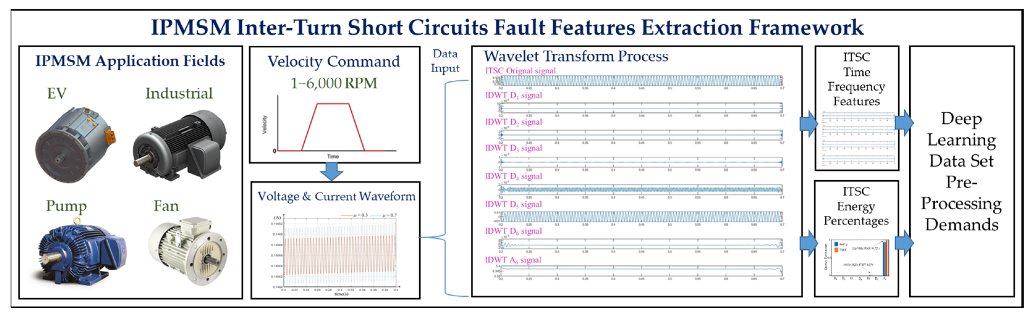
- Successfully established an IPMSM inter-turn short circuits fault feature extraction system framework, providing the data preprocessing required for designing deep learning models for motor failure analysis.
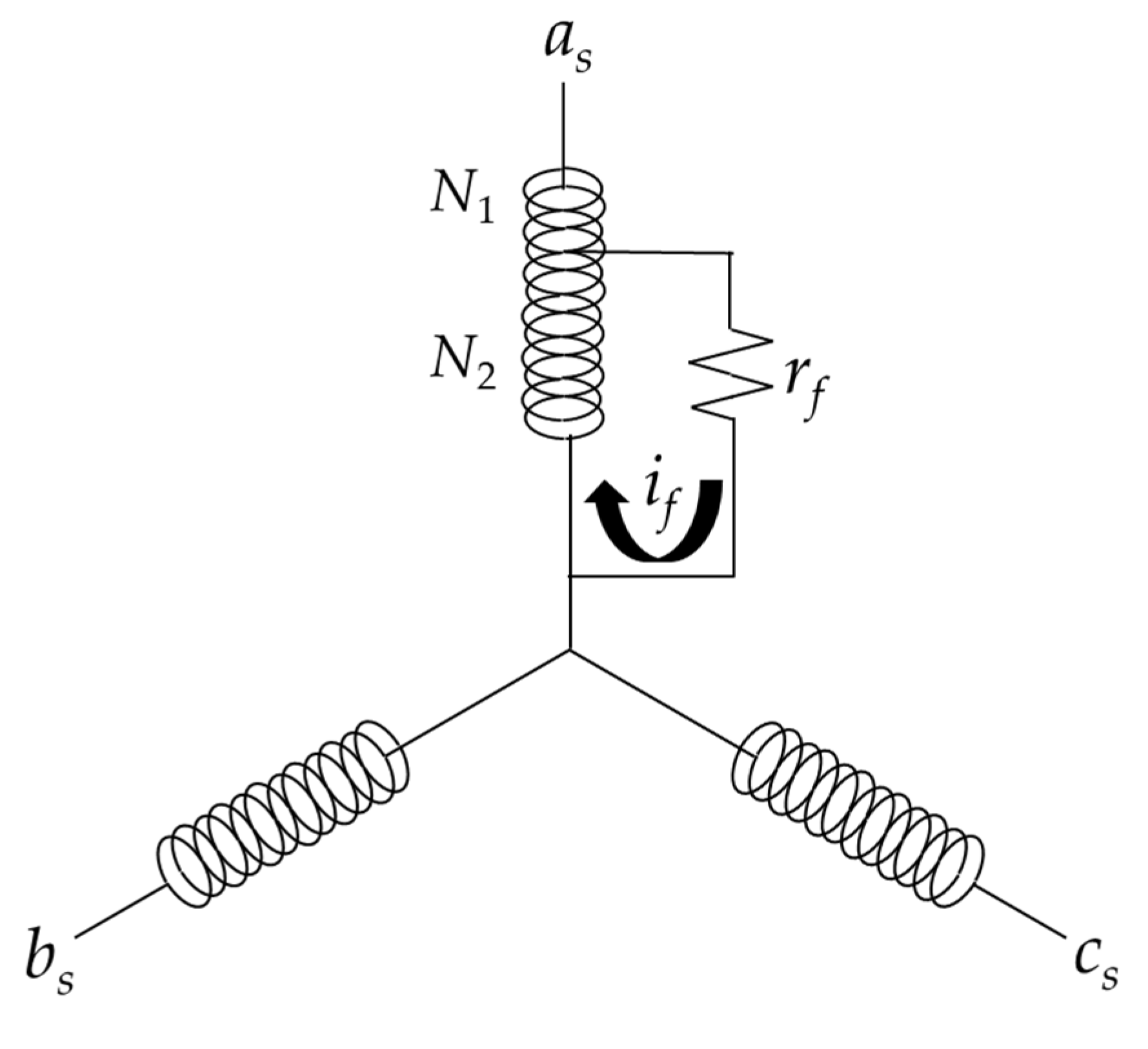
- Derived the physical model of the IPMSM ITSCF and successfully built simulation equations using MATLAB/Simulink/Simscape.
- Innovatively extracted ITSC fault features using wavelet transform, enabling the diagnosis of IPMSM ITSC failures.
- The proposed ITSC time-frequency features and ITSC energy level information can not only be used for motor fault diagnosis but also for determining the range of command failures based on energy characteristics.
2. Related Work
2.1. The Study of IPMSM Failures
2.2. Diagnosis Method Analysis
2.3. The Failure Models
3. ITSCF Model and Feature
3.1. The Pre-Processing System Framework
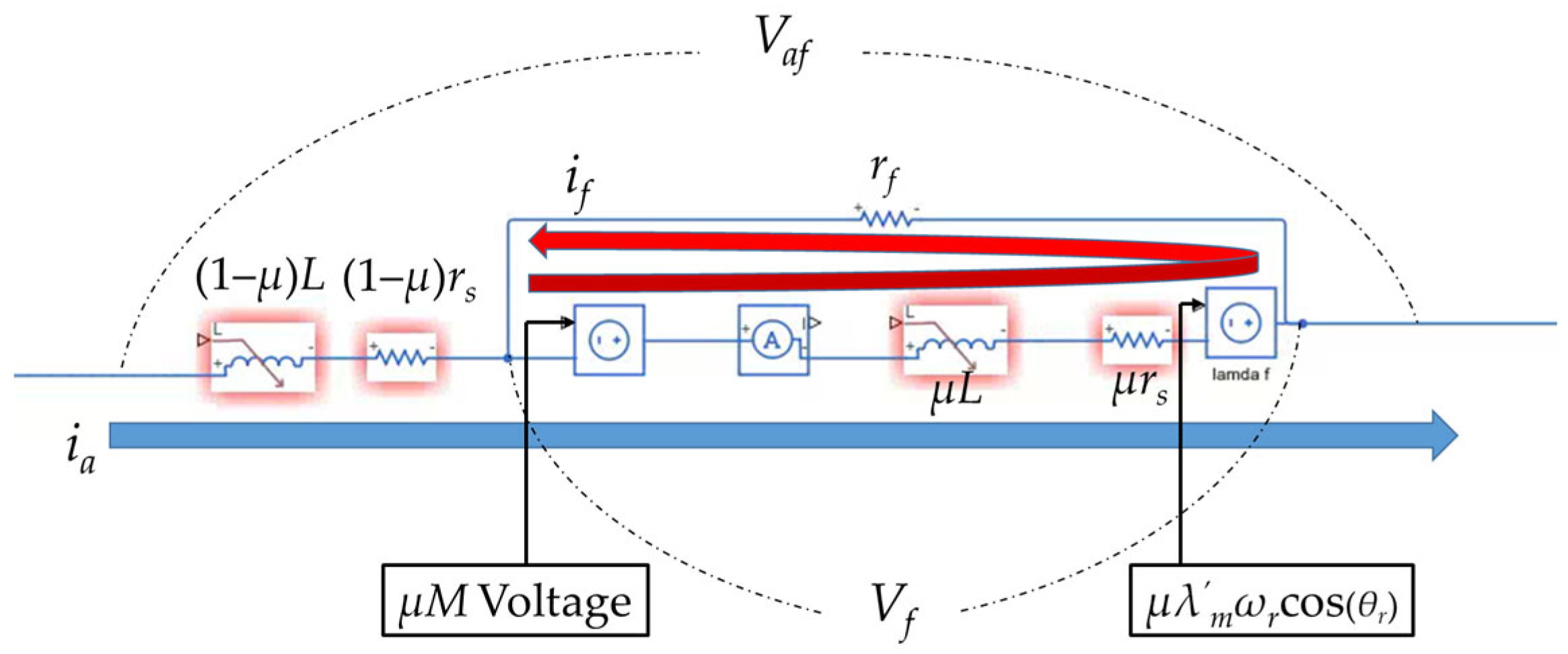
3.2. The Design of ITSCF Model
4. Wavelet Transform
4.1. Wavelet Transform Method
- Continuous Wavelet Transform
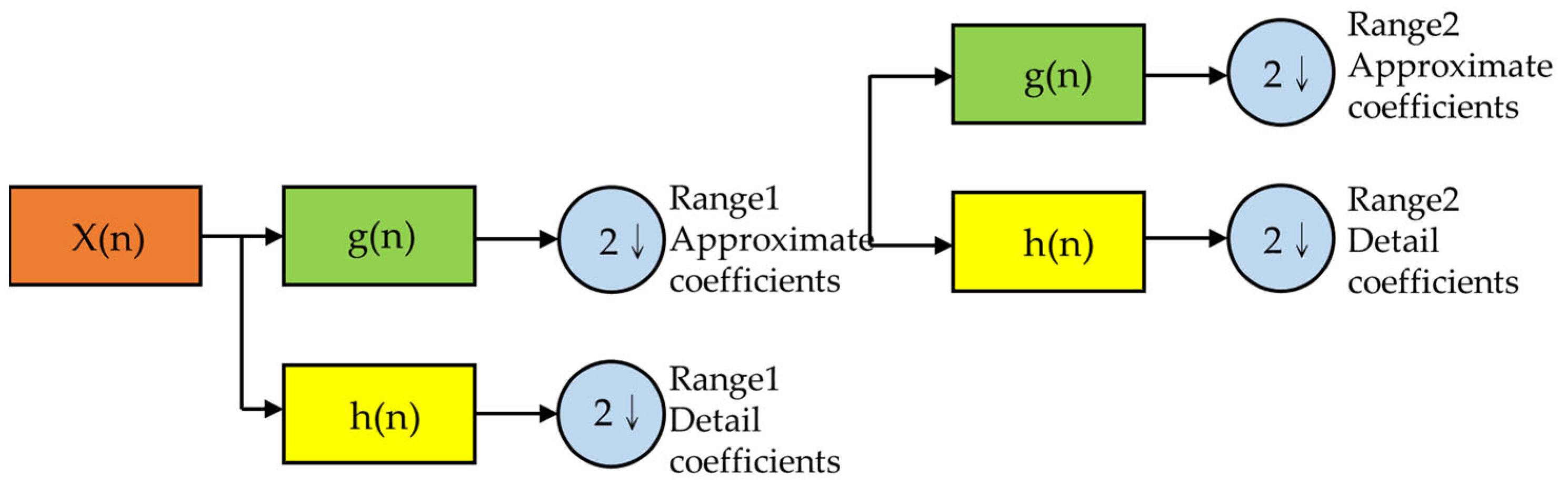
- Discrete Wavelet Transform
- DWT (Analysis)
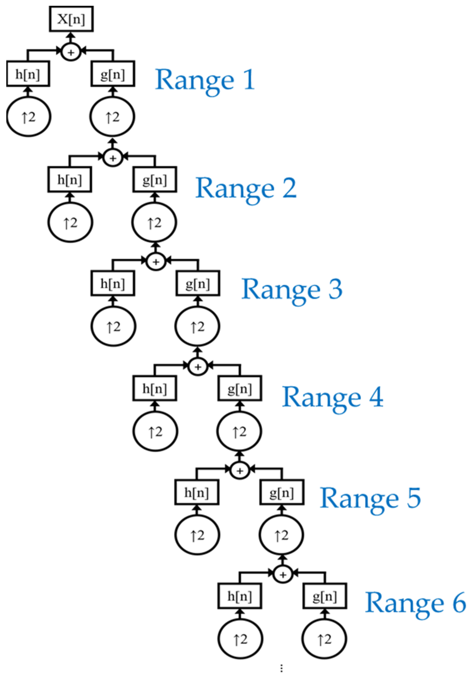
- IDWT (Synthesis)
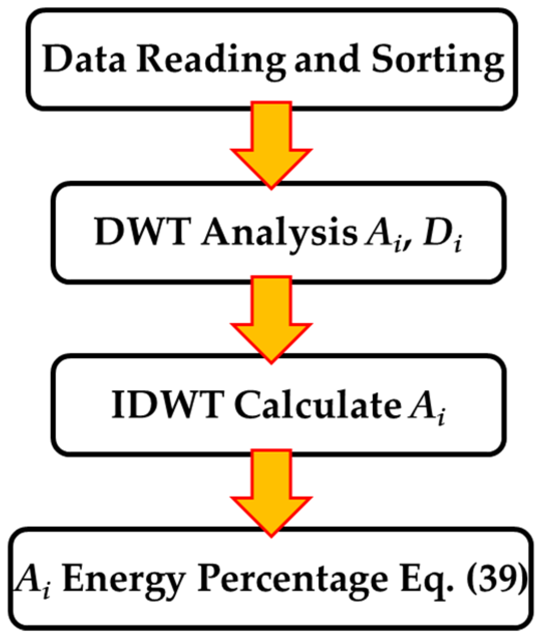
4.2. Implementation Process
5. Simulation Results
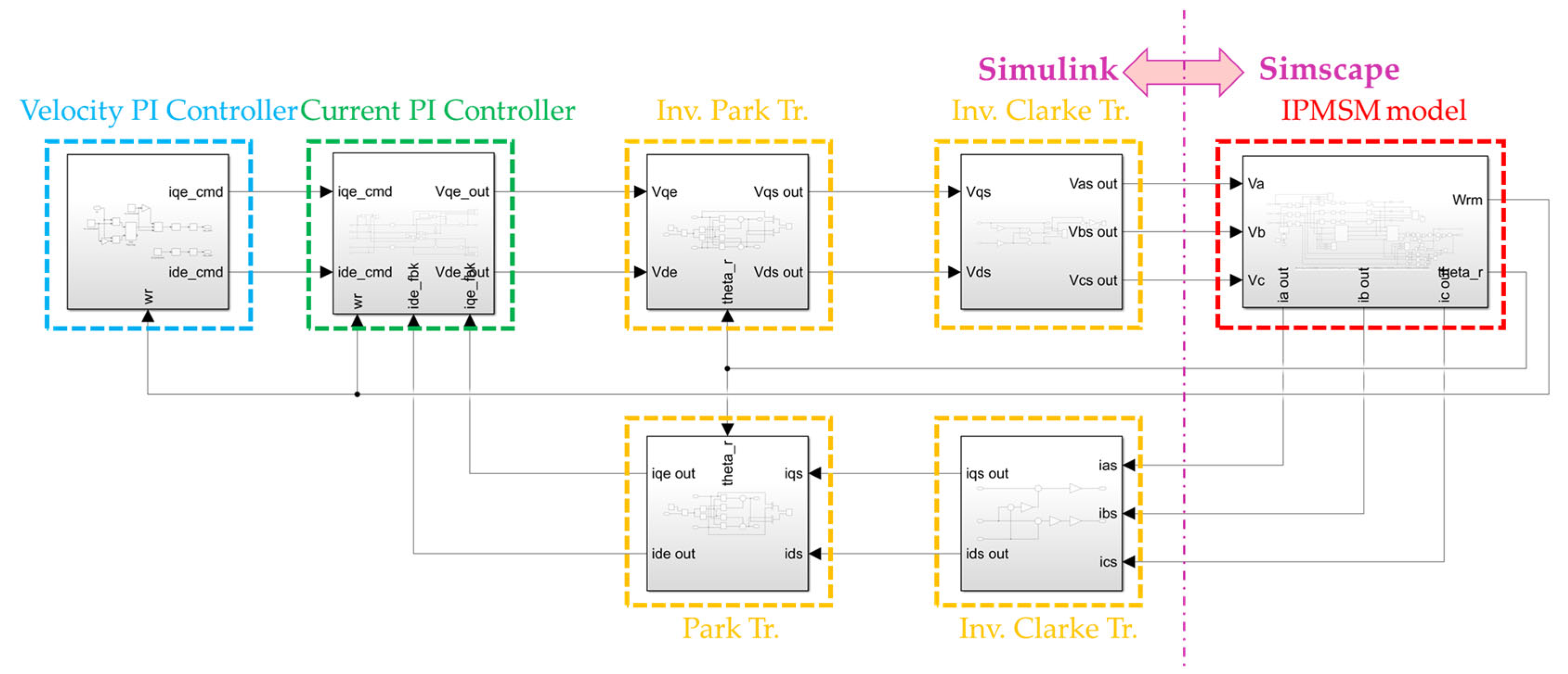
5.1. Simulation Platform
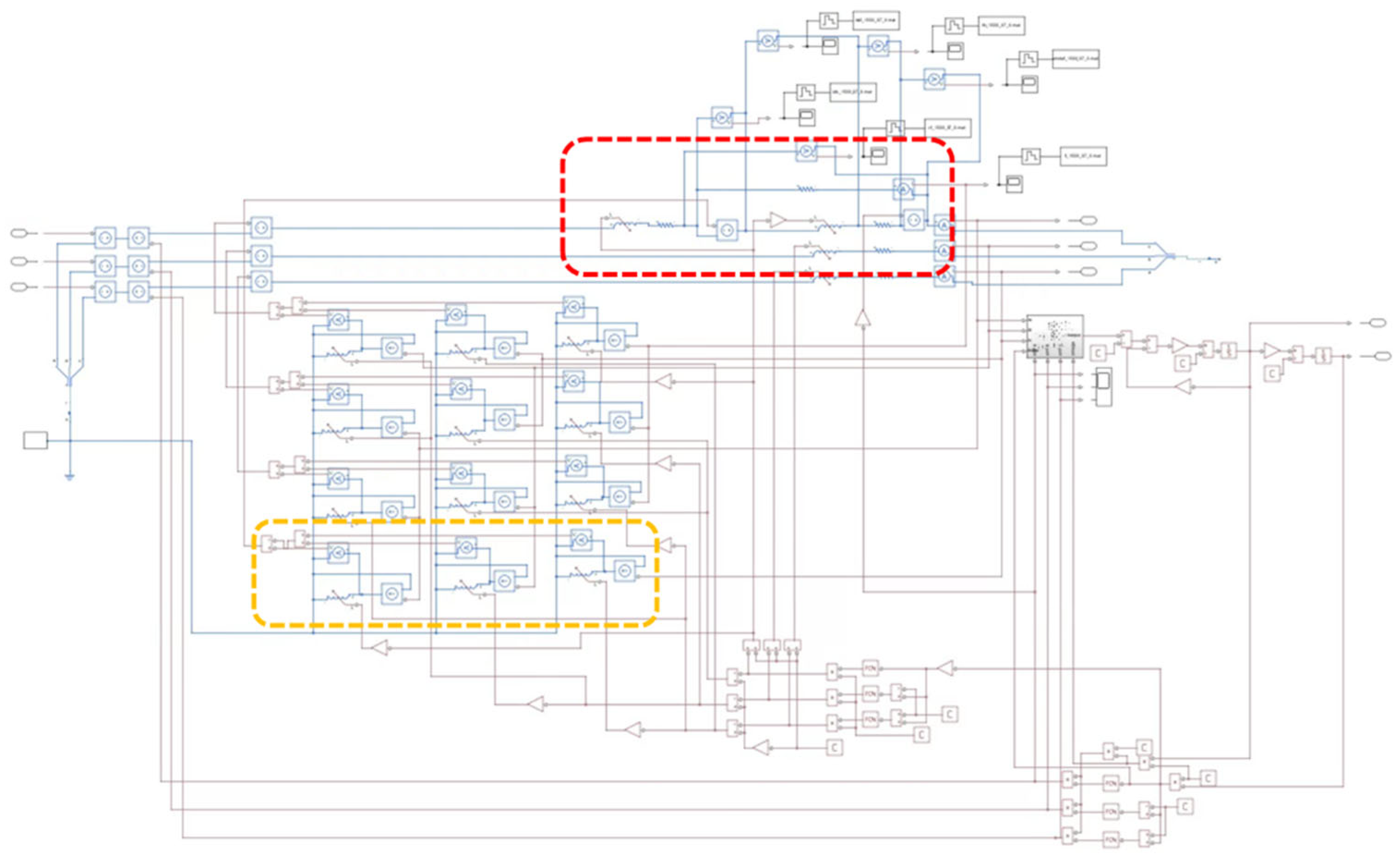
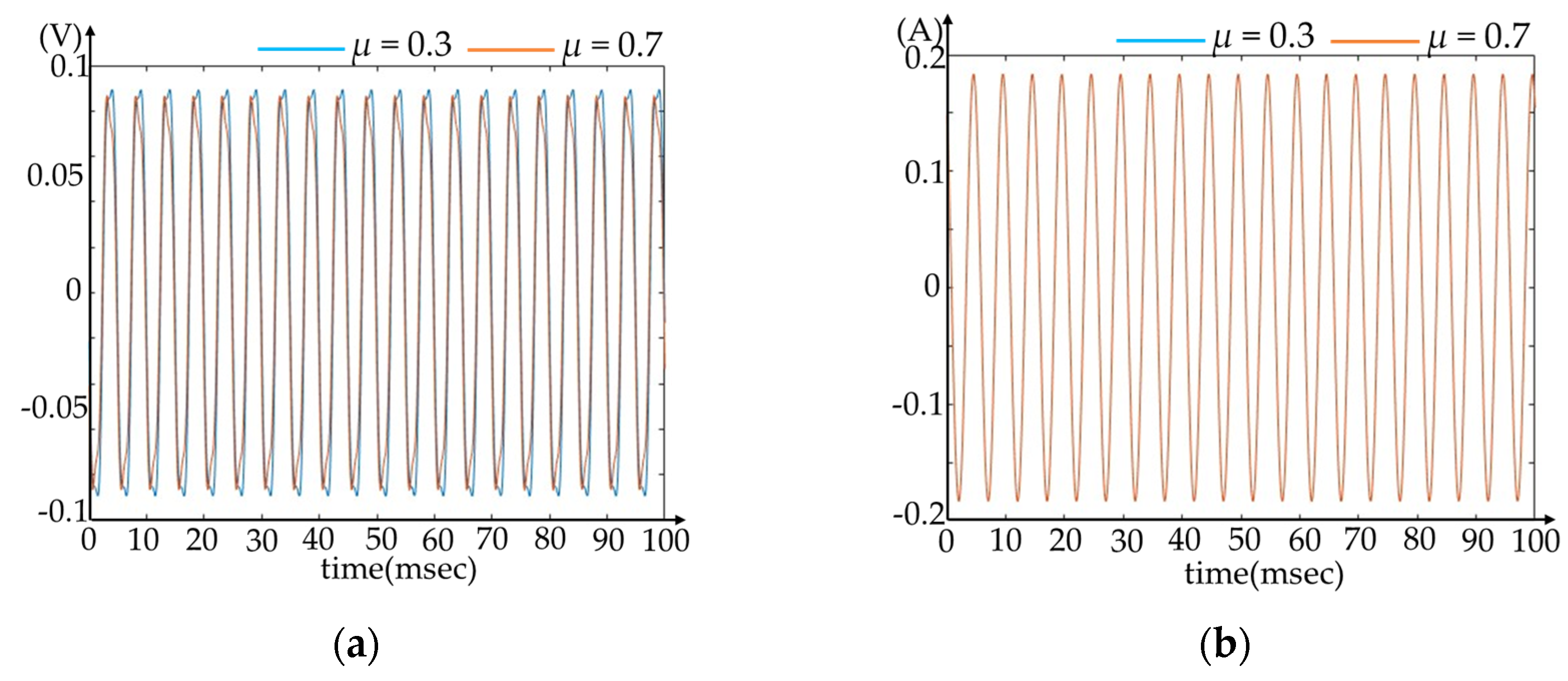
5.2. Simulation of the ITSCF Model
5.3. Wavelet Method Analysis Results
6. Experimental Results
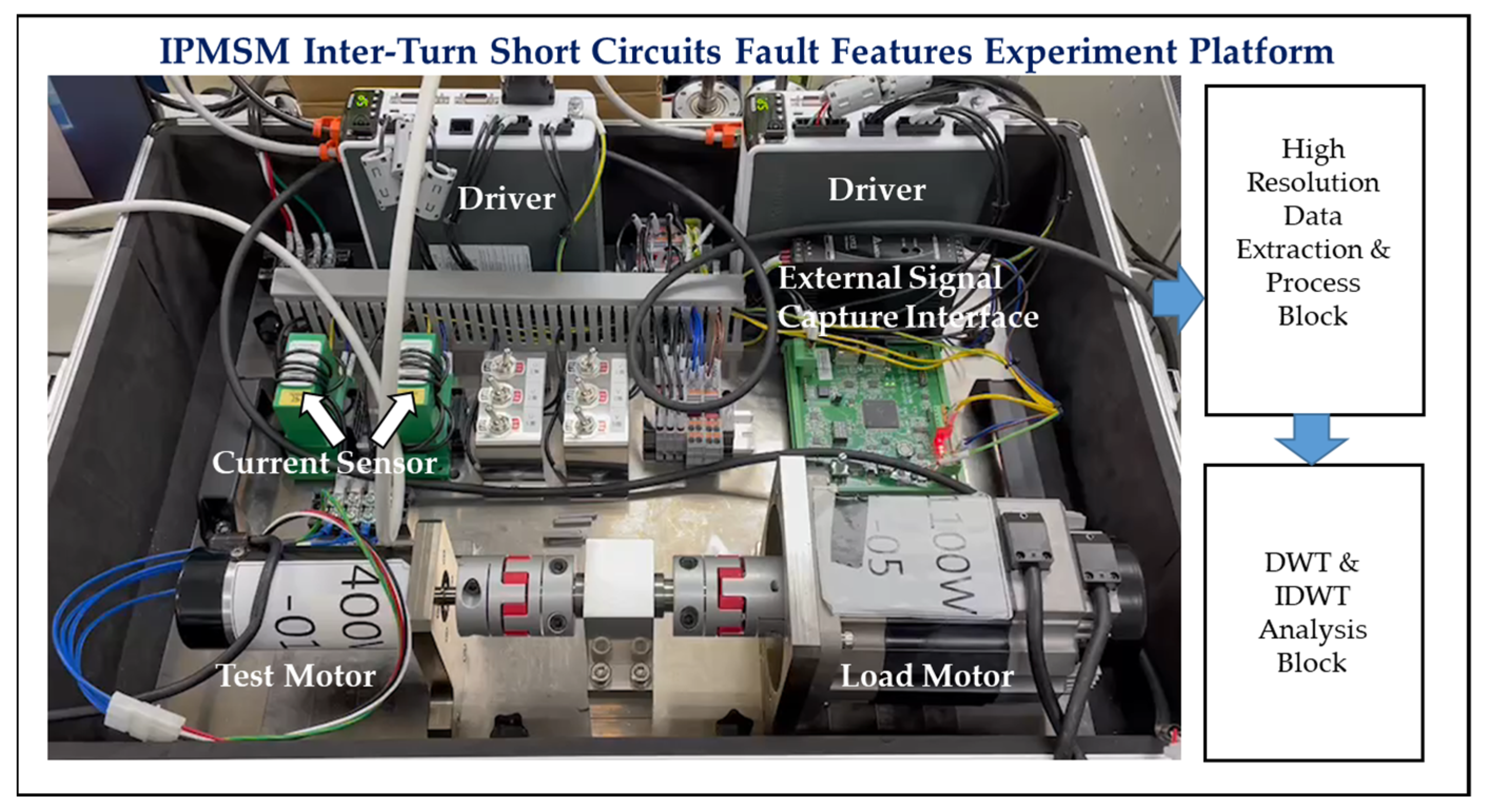
6.1. Experimental Platform
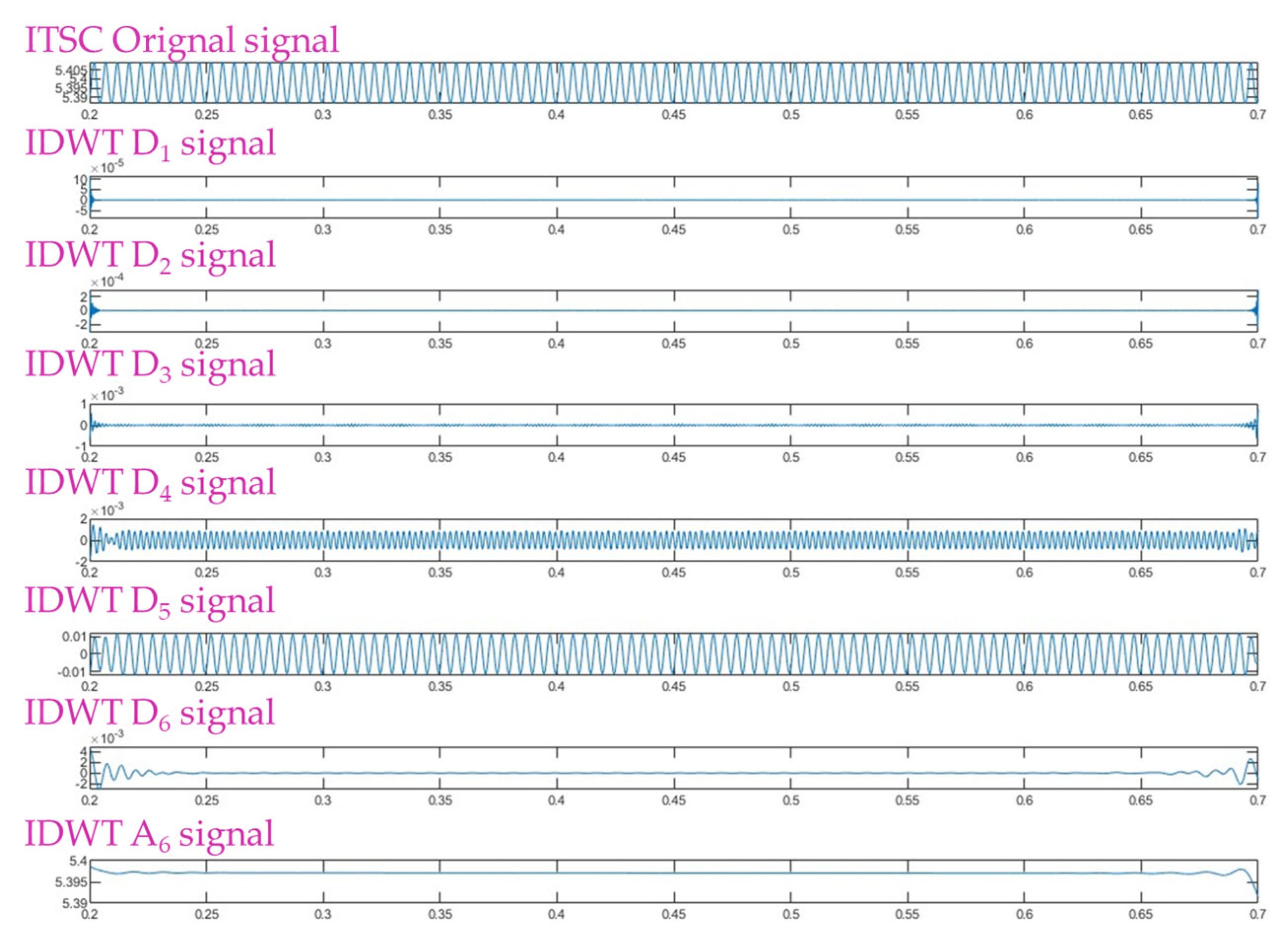
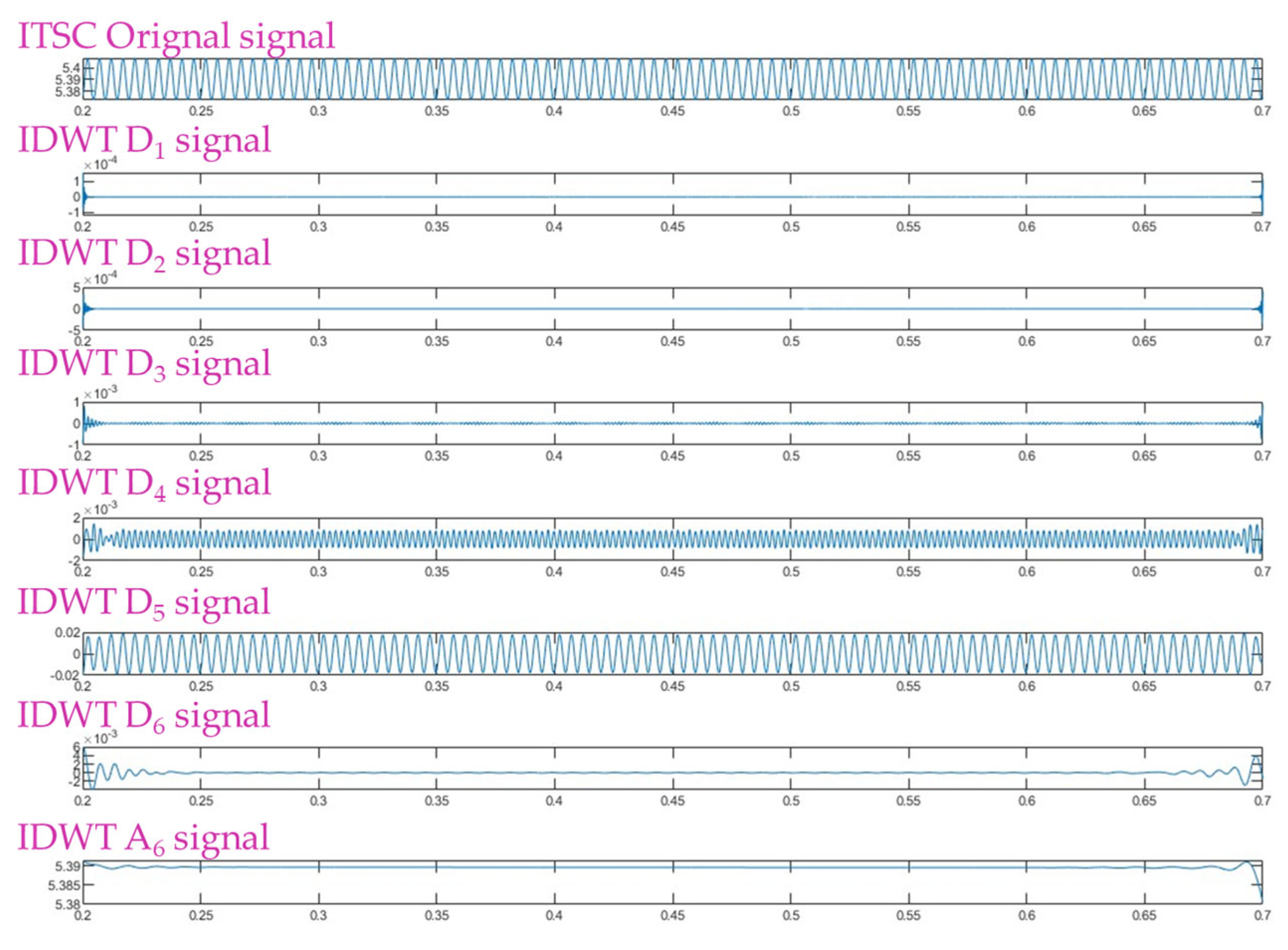
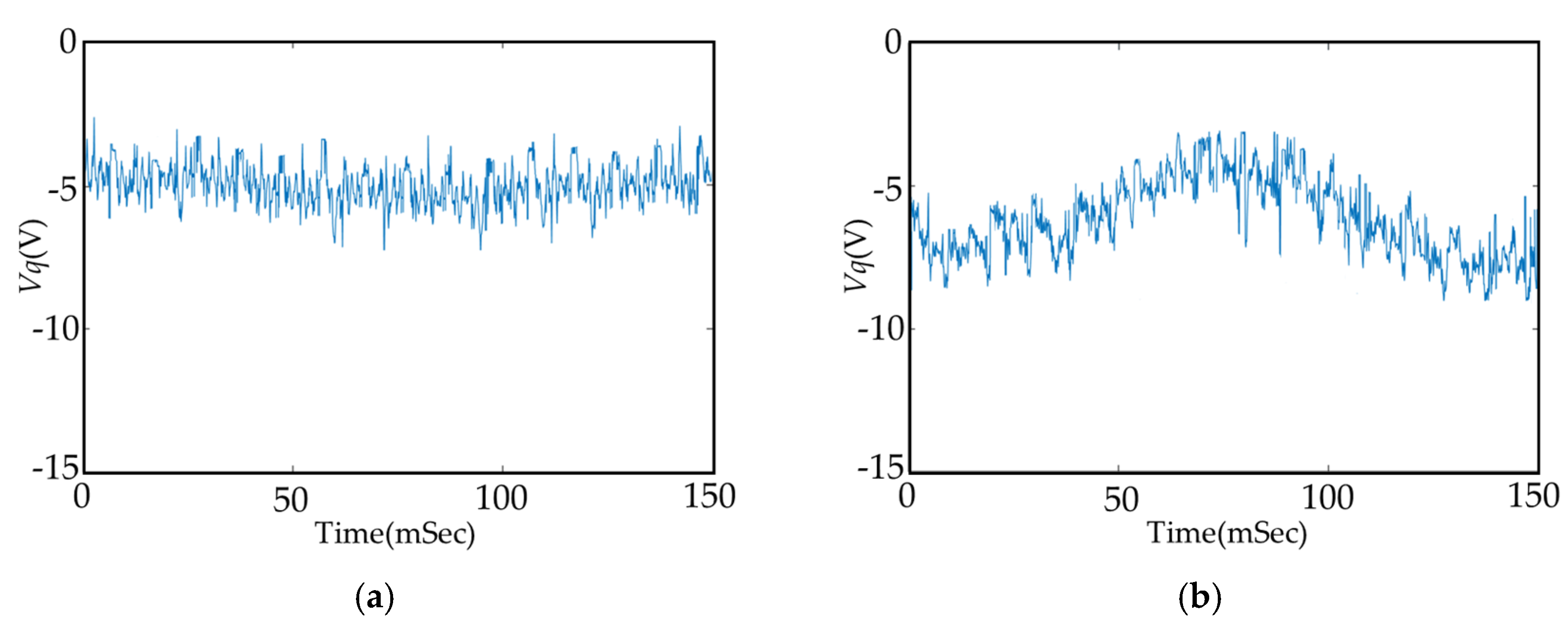
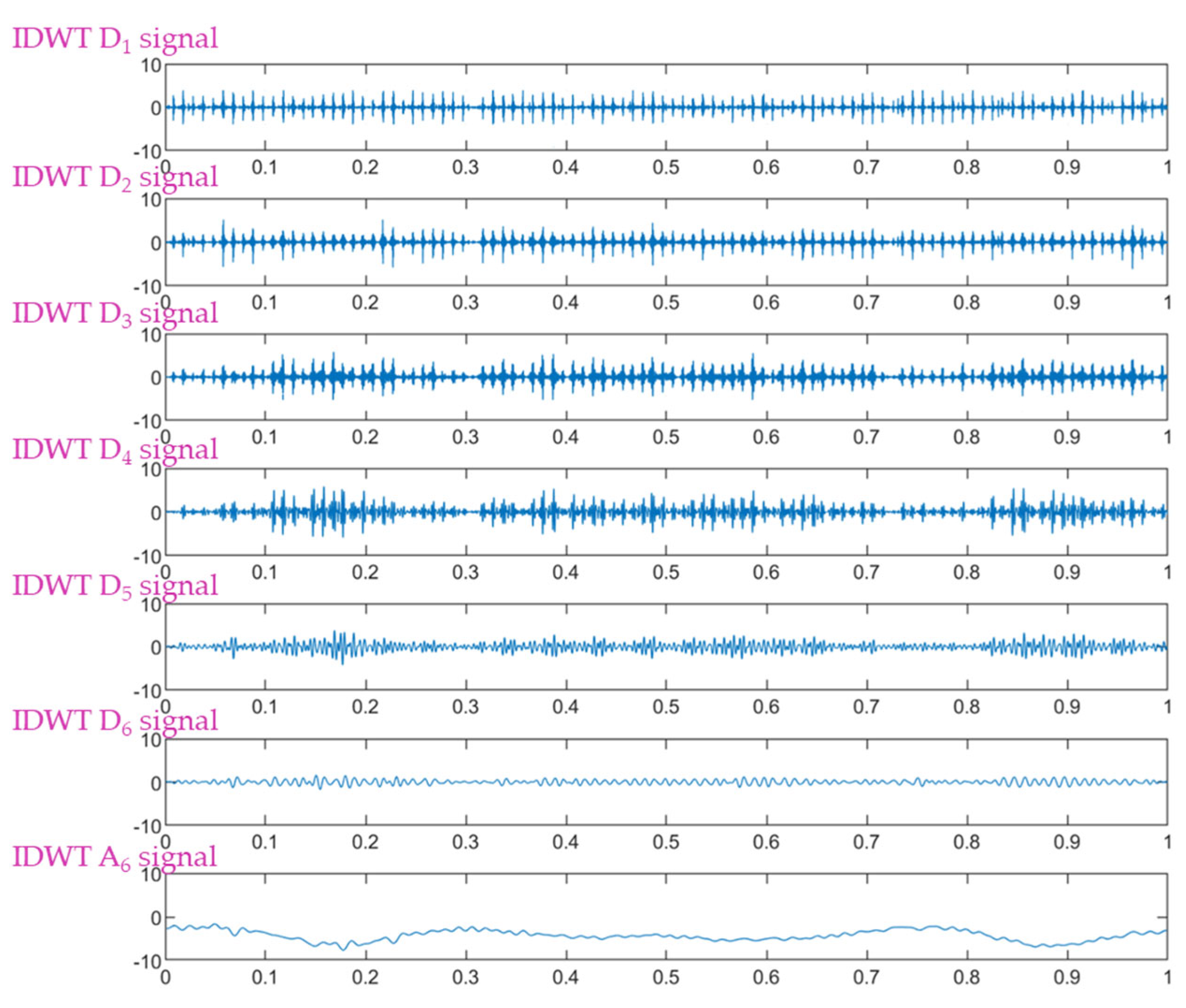
6.2. DWT Results
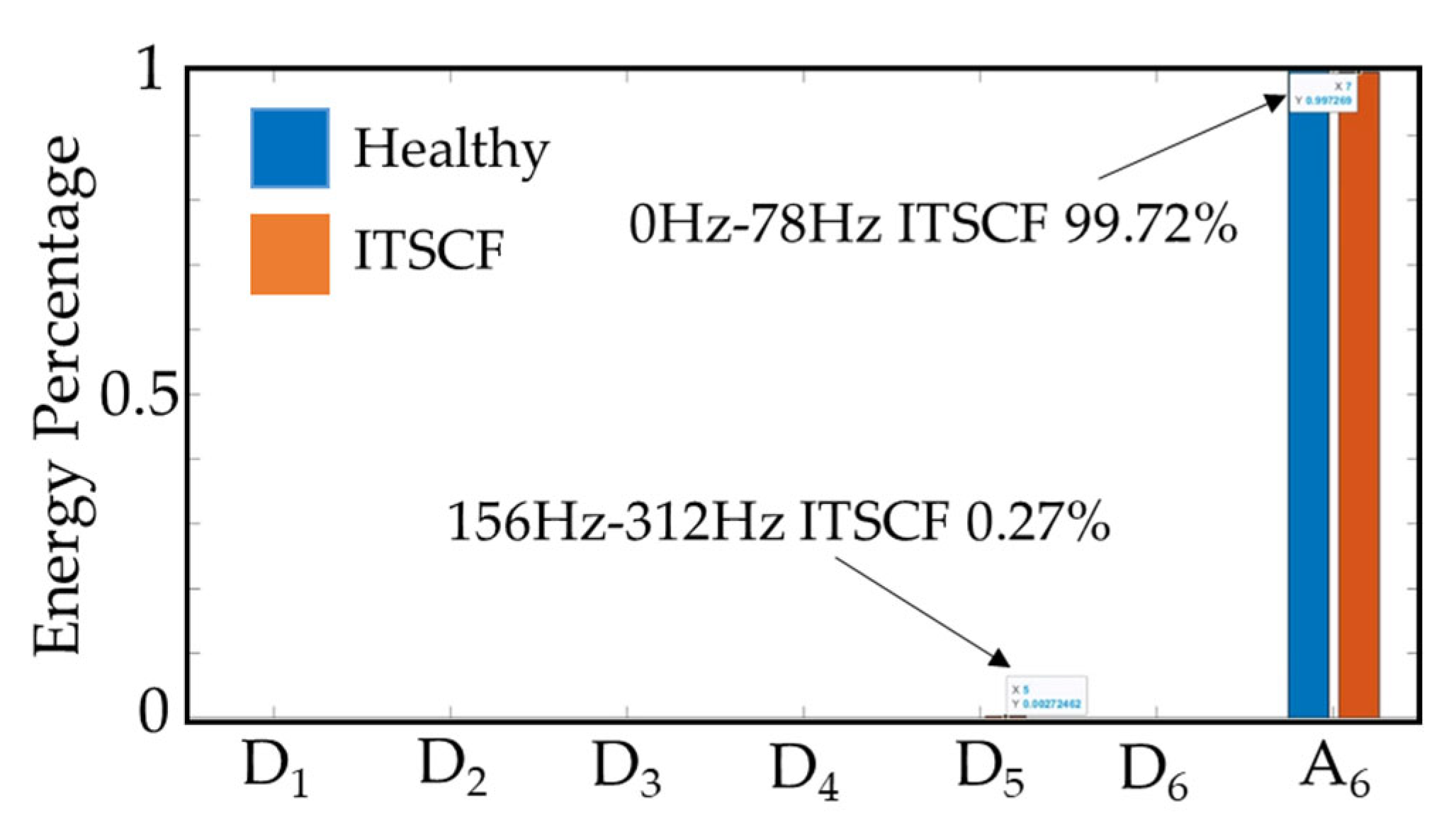
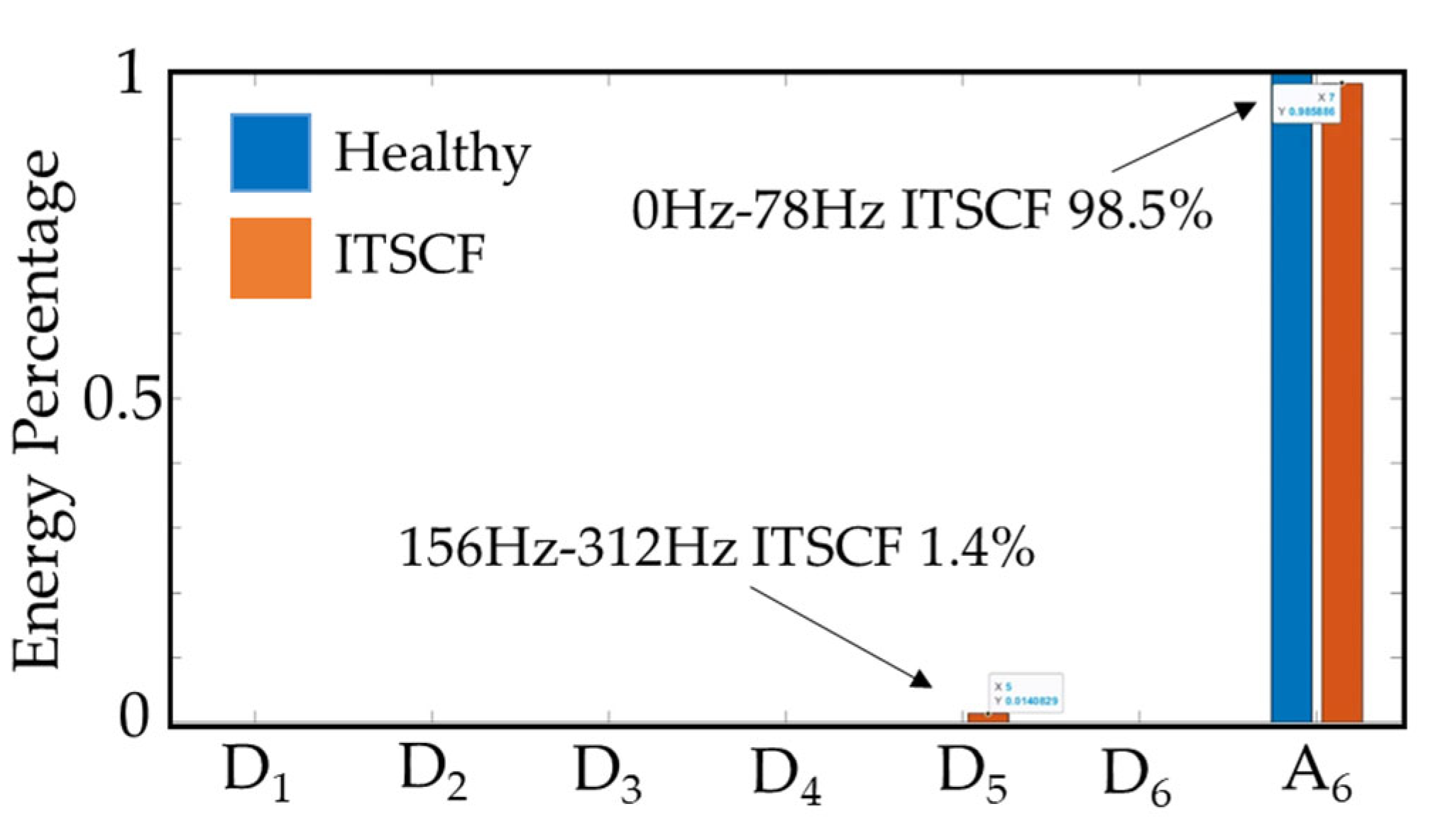
6.3. ITSCF Diagnosis Results
7. Conclusions and Discussion
Author Contributions
Funding
Institutional Review Board Statement
Informed Consent Statement
Data Availability Statement
Acknowledgments
Conflicts of Interest
References
- Amara, Y.; Barakat, G. Modeling and Diagnostic of Stator Faults in Induction Machines Using Permeance Network Method. In Proceedings of the PIERS Proceedings, Marrakesh, Morocco, 20–23 March 2011. [Google Scholar]
- Cherif, H.; Menacer, A.; Bessam, B.; Kechida, R. Stator Inter Turns Fault Detection Using Discrete Wavelet Transform. In Proceedings of the IEEE 10th International Symposium on Diagnostics for Electrical Machines, Power Electronics and Drives, Guarda, Portugal, 1–4 September 2015. [Google Scholar]
- Riera-Guasp, M.; Antonino-Daviu, J.A.; Pineda-Sanchez, M.; Puche-Panadero, R.; Perez-Cruz, J. A General Approach for the Transient Detection of Slip-Dependent Fault Components Based on the Discrete Wavelet Transform. IEEE Trans. Ind. Electron. 2008, 55, 4167–4180. [Google Scholar] [CrossRef]
- Schoen, R.R.; Habetler, T.G. Evaluation and Implementation of a System to Eliminate Arbitrary Load Effects in Current-Based Monitoring of Induction Machines. IEEE Trans. Ind. Appl. 1997, 33, 1571–1577. [Google Scholar] [CrossRef]
- Antonino-Daviu, J.A.; Riera-Guasp, M.; Folch, J.R.; Palomares, M.P.M. Validation of a New Method for the Diagnosis of Rotor Bar Failures via Wavelet Transformation in Industrial Induction Machines. IEEE Trans. Ind. Appl. 2006, 42, 990–996. [Google Scholar] [CrossRef]
- Antonino-Daviu, J.; Jover, P.; Riera-Guasp, M.; Roger-Folch, J.; Arkkio, A. DWT Analysis of Numerical and Experimental Data for the Diagnosis of Dynamic Eccentricities in Induction Motors. Mech. Syst. Signal Process. 2007, 21, 2575–2589. [Google Scholar] [CrossRef]
- Ruiz, J.-R.R.; Rosero, J.A.; Espinosa, A.G.; Romera, L. Detection of Demagnetization Faults in Permanent-Magnet Synchronous Motors Under Nonstationary Conditions. IEEE Trans. Magn. 2009, 45, 2961–2969. [Google Scholar] [CrossRef]
- Ahn, G.; Lee, J.; Park, C.H.; Youn, M.; Youn, B.D. Inter-turn Short Circuit Fault Detection in Permanent Magnet Synchronous Motors Based on Reference Voltage. In Proceedings of the 2019 IEEE 12th International Symposium on Diagnostics for Electrical Machines, Power Electronics and Drives, Toulouse, France, 27–30 August 2019. [Google Scholar]
- Niu, G.; Dong, X.; Chen, Y. Motor Fault Diagnostics Based on Current Signatures: A Review. IEEE Trans. Instrum. Meas. 2023, 72, 3520919. [Google Scholar] [CrossRef]
- Faiz, J.; Nejadi-Koti, H. Demagnetization Fault Indexes in Permanent Magnet Synchronous Motors—An Overview. IEEE Trans. Magn. 2015, 52, 8201511. [Google Scholar] [CrossRef]
- Usman, A.; Rajpurohit, B.S. Comprehensive Analysis of Demagnetization Faults in BLDC Motors Using Novel Hybrid Electrical Equivalent Circuit and Numerical Based Approach. IEEE Access 2019, 7, 147542–147552. [Google Scholar] [CrossRef]
- Kim, K.H. Simple Online Fault Detecting Scheme for Short-Circuited Turn in a PMSM Through Current Harmonic Monitoring. IEEE Trans. Ind. Electron. 2011, 58, 2565–2568. [Google Scholar] [CrossRef]
- Haddad, R.Z.; Strangas, E.G. On the Accuracy of Fault Detection and Separation in Permanent Magnet Synchronous Machines Using MCSA/MVSA and LDA. IEEE Trans. Energy Convers. 2016, 31, 924–934. [Google Scholar] [CrossRef]
- Hang, J.; Zhang, J.; Cheng, M.; Huang, J. Online Interturn Fault Diagnosis of Permanent Magnet Synchronous Machine Using Zero Sequence Components. IEEE Trans. Power Electron. 2015, 30, 6731–6741. [Google Scholar] [CrossRef]
- Duan, Y.; Toliyat, H. A Review of Condition Monitoring and Fault Diagnosis for Permanent Magnet Machines. In Proceedings of the IEEE Power & Energy Society General Meeting, San Diego, CA, USA, 22–26 July 2012. [Google Scholar]
- Aubert, B.; Régnier, J.; Caux, S.; Alejo, D. Kalman-Filter-Based Indicator for Online Interturn Short Circuits Detection in Permanent-Magnet Synchronous Generators. IEEE Trans. Ind. Electron. 2015, 62, 1921–1930. [Google Scholar] [CrossRef]
- Urresty, J.C.; Riba, J.R.; Romeral, L. Diagnosis of Interturn Faults in PMSMs Operating Under Nonstationary Conditions by Applying Order Tracking Filtering. IEEE Trans. Power Electron. 2013, 28, 507–515. [Google Scholar] [CrossRef]
- Seshadrinath, J.; Singh, B.; Panigrahi, B.K. Investigation of Vibration Signatures for Multiple Fault Diagnosis in Variable Frequency Drives Using Complex Wavelets. IEEE Trans. Power Electron. 2014, 29, 936–945. [Google Scholar] [CrossRef]
- Seshadrinath, J.; Singh, B.; Panigrahi, B.K. Vibration Analysis Based Interturn Fault Diagnosis in Induction Machines. IEEE Trans. Ind. Inform. 2014, 10, 340–350. [Google Scholar] [CrossRef]
- Isermann, R. Fault-Diagnosis Applications; Springer: Berlin, Germany, 2011. [Google Scholar]
- Sarikhani, A.; Mohammed, O.A. Inter-Turn Fault Detection in PM Synchronous Machines by Physics-Based Back Electromotive Force Estimation. IEEE Trans. Ind. Electron. 2013, 60, 3472–3484. [Google Scholar] [CrossRef]
- De Angelo, C.H.; Bossio, G.R.; Giaccone, S.J.; Valla, M.I.; Solsona, J.A.; Garcia, G.O. Online Model-Based Stator-Fault Detection and Identification in Induction Motors. IEEE Trans. Ind. Electron. 2009, 56, 4671–4680. [Google Scholar] [CrossRef]
- Romeral, L.; Urresty, J.C.; Riba Ruiz, J.R.; Garcia Espinosa, A. Modeling of Surface-Mounted Permanent Magnet Synchronous Motors with Stator Winding Interturn Faults. IEEE Trans. Ind. Electron. 2011, 58, 1576–1585. [Google Scholar] [CrossRef]
- Jeong, I.; Hyon, B.J.; Nam, K. Dynamic Modeling and Control for SPMSMs with Internal Turn Short Fault. IEEE Trans. Power Electron. 2013, 28, 3495–3508. [Google Scholar] [CrossRef]
- Gu, B.G. Study of IPMSM Interturn Faults—Part I: Development and Analysis of Models with Series and Parallel Winding Connections. IEEE Trans. Power Electron. 2016, 31, 5931–5943. [Google Scholar] [CrossRef]
- Obeid, N.H.; Boileau, T.; Nahid-Mobarakeh, B. Modeling and Diagnostic of Incipient Interturn Faults for a Three-Phase Permanent Magnet Synchronous Motor. IEEE Trans. Ind. Appl. 2016, 52, 4426–4434. [Google Scholar] [CrossRef]
- Bouzid, M.B.K.; Champenois, G.; Bellaaj, N.M.; Signac, L.; Jelassi, K. An Effective Neural Approach for the Automatic Location of Stator Interturn Faults in Induction Motor. IEEE Trans. Ind. Electron. 2008, 55, 4277–4289. [Google Scholar] [CrossRef]
- Patil, P.; Mane, S.B.; Dhamija, L. Detection of Inter-Turn Short Circuit in Permanent Magnet Synchronous Motor using Machine Learning. In Proceedings of the International Conference on Signal and Information Processing, Virtual, 7–8 December 2022. [Google Scholar]
- Shih, K.J.; Hsieh, M.F.; Chen, B.J.; Huang, S.F. Machine Learning for Inter-Turn Short-Circuit Fault Diagnosis in Permanent Magnet Synchronous Motors. IEEE Trans. Magn. 2022, 58, 8204307. [Google Scholar] [CrossRef]
- Fang, Y.; Wang, M.; Wei, L. Deep Transfer Learning in Inter-turn Short Circuit Fault Diagnosis of PMSM. In Proceedings of the IEEE International Conference on Mechatronics and Automation, Takamatsu, Japan, 8–11 August 2021. [Google Scholar]
- Gaber, I.M.; Shalash, O.; Hamad, M.S. Optimized Inter-Turn Short Circuit Fault Diagnosis for Induction Motors using Neural Networks with LeLeRU. In Proceedings of the IEEE Conference on Power Electronics and Renewable Energy, Luxor, Egypt, 19–21 February 2023. [Google Scholar]
- Jung, W.; Yun, S.H.; Lim, Y.S.; Cheong, S.; Bae, J.; Park, Y.H. Fault Diagnosis of Inter-turn Short Circuit in Permanent Magnet Synchronous Motors with Current Signal Imaging and Semi-Supervised Learning. In Proceedings of the Annual Conference of the IEEE Industrial Electronics Society, Brussels, Belgium, 17–20 October 2022. [Google Scholar]


| Quantity | Value | Units |
|---|---|---|
| Rated Voltage | 48 | V |
| Rated Current | 9 | A |
| Rated Power | 400 | W |
| Rated Torque | 600 | mNm |
| Max. Speed | 6000 | rpm |
| Poles (P) | 8 | pole |
| Stator Resistance (rs) | 0.33 | Ω |
| q-axis Inductance (Lq) | 1.2606 | mH |
| d-axis Inductance (Ld) | 1.0045 | mH |
| PM Flux Linkage (λm) | 0.008625 | Wb |
| Rotor Inertia (Jm) | 0.0001 | kg·m2 |
| Damping (Bm) | 0.0000484 | N·m·s−1 |
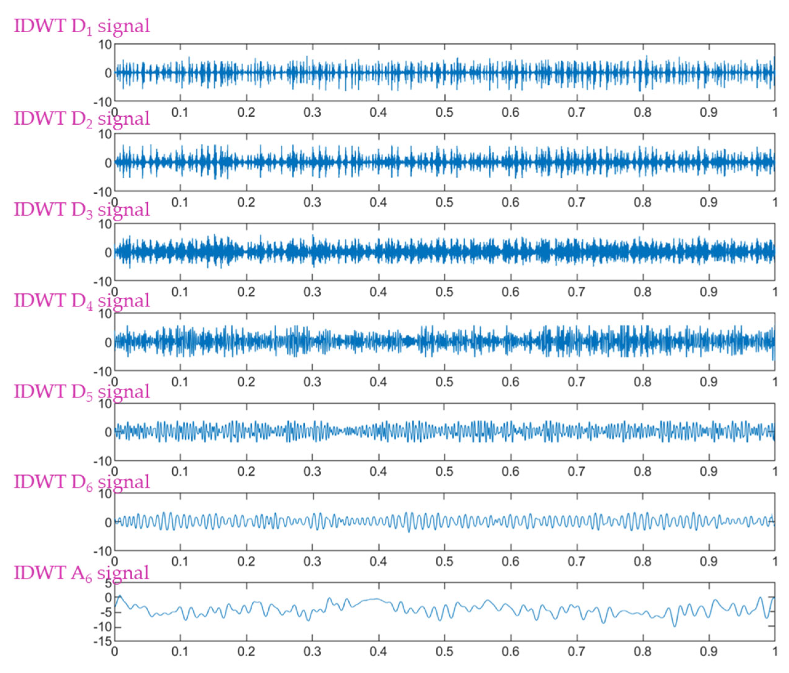
| DWT Coefficient | Symbol | Frequency Range |
|---|---|---|
| Detailed Coefficient of the First Range | D1 | 2500~5000 Hz |
| Detailed Coefficient of the Second Range | D2 | 1250~2500 Hz |
| Detailed Coefficient of the Third Range | D3 | 625~1250 Hz |
| Detailed Coefficient of the Fourth Range | D4 | 312~625 Hz |
| Detailed Coefficient of the Fifth Range | D5 | 156~312 Hz |
| Detailed Coefficient of the Sixth Range | D6 | 78~156 Hz |
| Approximate Coefficient of the Sixth Range | A6 | 0~78 Hz |
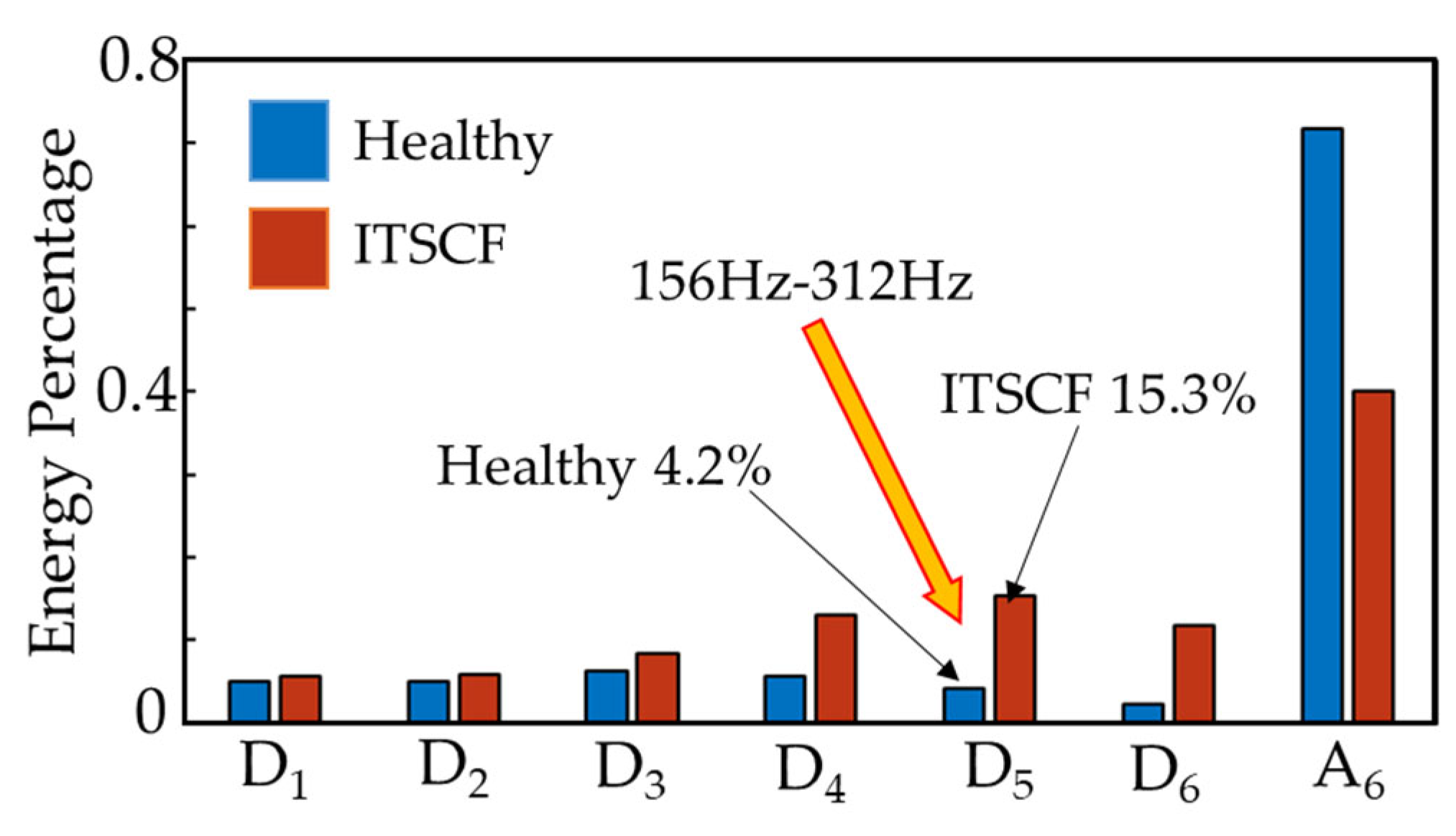
| Frequency Range | Healthy Condition | ITSCF |
|---|---|---|
| 2500~5000 Hz | 5.0% | 5.7% |
| 1250~2500 Hz | 5.0% | 5.8% |
| 625~1250 Hz | 6.3% | 8.3% |
| 312~625 Hz | 5.7% | 13.1% |
| 156~312 Hz | 4.2% | 15.3% |
| 78~156 Hz | 2.2% | 11.7% |
| 0~78 Hz | 71.8% | 40.1% |
| DWT Coefficient | Symbol | Frequency Range |
|---|---|---|
| Detailed Coefficient of the First Range | D1 | 7500~3750 Hz |
| Detailed Coefficient of the Second Range | D2 | 3750~1875 Hz |
| Detailed Coefficient of the Third Range | D3 | 1875~937 Hz |
| Detailed Coefficient of the Fourth Range | D4 | 937~468 Hz |
| Detailed Coefficient of the Fifth Range | D5 | 468~234 Hz |
| Detailed Coefficient of the Sixth Range | D6 | 234~117 Hz |
| Detailed Coefficient of the Seventh Range | D7 | 117~58 Hz |
| Approximate Coefficient of the Seventh Range | A7 | 58~0 Hz |
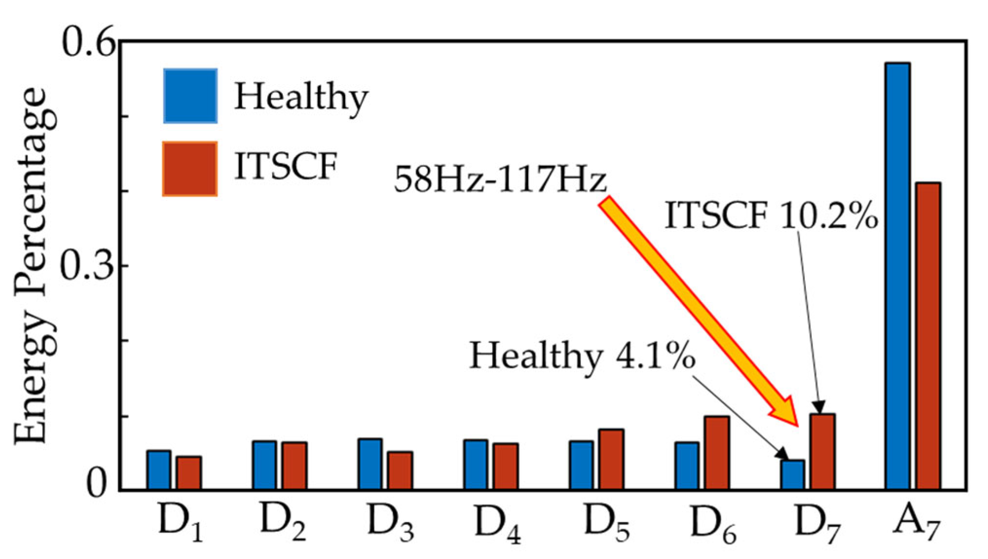
| Frequency Range | Healthy | ITSCF |
|---|---|---|
| 7500~3750 Hz | 5.3% | 4.6% |
| 3750~1875 Hz | 6.6% | 6.4% |
| 1875~937 Hz | 7.0% | 5.1% |
| 937~468 Hz | 6.8% | 6.3% |
| 468~234 Hz | 6.7% | 8.3% |
| 234~117 Hz | 6.5% | 9.9% |
| 117~58 Hz | 4.1% | 10.2% |
| 58~0 Hz | 57.1% | 41.2% |
Disclaimer/Publisher’s Note: The statements, opinions and data contained in all publications are solely those of the individual author(s) and contributor(s) and not of MDPI and/or the editor(s). MDPI and/or the editor(s) disclaim responsibility for any injury to people or property resulting from any ideas, methods, instructions or products referred to in the content. |
© 2024 by the authors. Licensee MDPI, Basel, Switzerland. This article is an open access article distributed under the terms and conditions of the Creative Commons Attribution (CC BY) license (https://creativecommons.org/licenses/by/4.0/).
Share and Cite
Chen, C.-S.; Lin, C.-J.; Yang, F.-J.; Lin, F.-C. Model Design of Inter-Turn Short Circuits in Internal Permanent Magnet Synchronous Motors and Application of Wavelet Transform for Fault Diagnosis. Appl. Sci. 2024, 14, 9570. https://doi.org/10.3390/app14209570
Chen C-S, Lin C-J, Yang F-J, Lin F-C. Model Design of Inter-Turn Short Circuits in Internal Permanent Magnet Synchronous Motors and Application of Wavelet Transform for Fault Diagnosis. Applied Sciences. 2024; 14(20):9570. https://doi.org/10.3390/app14209570
Chicago/Turabian StyleChen, Chin-Sheng, Chia-Jen Lin, Fu-Jen Yang, and Feng-Chieh Lin. 2024. "Model Design of Inter-Turn Short Circuits in Internal Permanent Magnet Synchronous Motors and Application of Wavelet Transform for Fault Diagnosis" Applied Sciences 14, no. 20: 9570. https://doi.org/10.3390/app14209570
APA StyleChen, C.-S., Lin, C.-J., Yang, F.-J., & Lin, F.-C. (2024). Model Design of Inter-Turn Short Circuits in Internal Permanent Magnet Synchronous Motors and Application of Wavelet Transform for Fault Diagnosis. Applied Sciences, 14(20), 9570. https://doi.org/10.3390/app14209570