Article

Design and Research of a Virtual Laboratory for Coding Theory

Faculty of Electrical Engineering, Electronics and Automation, University of Ruse “Angel Kanchev”, 7017 Ruse, Bulgaria
*
Author to whom correspondence should be addressed.
Appl. Sci. 2024, 14(20), 9546; https://doi.org/10.3390/app14209546
Submission received: 2 September 2024 / Revised: 14 October 2024 / Accepted: 16 October 2024 / Published: 19 October 2024

Abstract

:
This article examines the process of creating and researching a virtual laboratory for training students in coding theory. General information about the virtual laboratories is presented. A methodology for conducting comprehensive scientific research is presented, as well as a specialized method for designing and developing the virtual laboratory, including the system’s architecture. The article also presents brief information about the developed system. The results of the experimental research, including a pedagogical experiment aimed at evaluating the influence of the virtual laboratory on the students’ success rate, as well as an analysis of the statistical data on their activity, are discussed in detail. In addition, a survey was conducted to assess the satisfaction of students with the use of the laboratory.

1. Introduction

Virtual laboratories are becoming increasingly common as an innovative educational toolkit that is successfully used in the educational process in various academic courses and diverse learning situations [1,2,3,4]. Creating a virtual laboratory for teaching and learning is complex, requiring skills in miscellaneous areas such as interaction design, visualization, and pedagogy. Different research groups, university teams, and even industry representatives have developed their own virtual laboratories covering a very wide area of disciplines [5,6,7,8,9,10,11].
The two most common types of virtual labs are virtual labs based on real equipment and virtual labs based on software simulators [12]. From the perspective of end users, they look very similar, providing a virtual service accessible through either a web interface or a client application, but there is a big difference in the programming technologies for their implementation [4,12,13]. In the remote laboratory, all hardware components (for example, measuring equipment) exist physically in the educational institution. By connecting this equipment to the network, the experiment can be controlled and studied by students at a remote location. Because real equipment is accessed, experiments are conducted on a predetermined schedule. In the virtual lab, all the above components are fully simulated with software tools and can be accessed anytime and anywhere by the users.
From the perspective of the university teacher, virtual and remote laboratories provide an opportunity to break out of the physical limitations of the traditional laboratory and make exercises available to a wider audience of students over a wider range of time. As these labs use information and communication technology, it is possible to track student activity and progress and collect statistics that can be used to generate useful feedback on the effectiveness of a virtual or remote lab and also to identify problems with a given learning material [12]. From the students’ point of view, the most attractive advantages are the possibility of conducting an experiment independently and the accessibility of the laboratory at any time and from anywhere. The main drawback of virtual and remote laboratories is the lack of physical contact with the devices and equipment; therefore, these laboratories do not improve practical skills, i.e., the dexterity required to achieve the same result of the experiment when operating the equipment in real conditions. This effect can be reduced to some extent by using high-quality 3D models of the equipment. Another drawback arises from the fact that the virtual environment is similar to video games, and students develop a tendency to perceive the virtual experiment as a game; therefore, they do not understand the seriousness of the experiment being studied. In remote labs, students are less likely to cause damage and cannot get hurt when they make mistakes because all controlled components have limits predetermined and checked by the software environment. These labs do not require the same level of discipline and caution that is needed to conduct the experiment in a traditional lab in a safe manner [12].
The implementation of the virtual laboratory is associated with lower costs since no real expensive equipment is used. Virtual lab hardware does not age or wear out as much as real equipment does, resulting in lower maintenance costs. It is also significantly cheaper to develop a new experiment, as there is no need to purchase new equipment. Virtual laboratories allow conducting a variety of virtual (simulation) experiments involving various components (virtual apparatus), including dangerous experiments [14]. Some laboratory experiments are dangerous; therefore, a teacher must be present in the laboratory, and the necessary theoretical knowledge of the student must be tested before starting [13]. Another advantage of virtual laboratories is the possibility of conducting experiments that are difficult to implement in real conditions. In a virtual laboratory, students can safely conduct experiments by simulating extreme conditions. For example, changes to the system configuration can be made and various system parameters can be modified. Such changes in most cases cannot be made with the actual equipment. Virtual laboratories provide an opportunity to learn from mistakes, as they provide opportunities for various tests and experiments that cannot be tested with real equipment [12].
Various examples of virtual laboratories for studying coding theory can be cited. In the research by [15], a Java-based virtual laboratory for data communication simulation is presented. The authors conclude that it is useful to facilitate the understanding of students taking courses in Communication Systems. A remotely accessible laboratory for error-controlled coding techniques with the LabVIEW software is presented in [16]. Students connect to the laboratory site and can perform different experiments and also access theoretical information. In the study by [17], students were formed into two groups (control and experimental groups) to evaluate the success of the virtual laboratory for digital electronics. The students in the experimental group used the developed virtual laboratory, while the students in the control group did not use it. The comparison process was carried out based on 10 different criteria.

2. Materials and Methods

For the research and creation of a coding theory virtual laboratory, an appropriate methodology is Action Research, introduced by Kurt Lewin and John Collier in the 1940s [18]. This methodology is often used in the field of education [19,20] and allows not only to analyze and evaluate the effects of the implementation of the virtual laboratory on the success of students but also to make practical changes in real time, based on continuous feedback from the participants [21]. Figure 1 shows the scientific methodology used in the study, which consists of 5 stages.
  • Stage 1. Problem Identification and Planning.
    o
    Problem Identification. The research problem originates from the need to improve students’ practical skills and understanding, as well as to overcome the lack of motivation in using the traditional written teaching method by implementing intuitive interactive software models for solving coding theory tasks. Another good reason for the creation of such a system is the need to provide a tool for working in the conditions of distance learning, as was the situation with COVID-19 [22].
    o
    Formulating the Goal. The purpose of the research is to create and examine the impact of using a coding theory virtual lab on student achievement and engagement.
    o
    Action Planning. For the purpose of the research, two groups of students will be formed: the control group (the students in this group solve the tasks according to the traditional written method) and the experimental group (the students in this group solve the tasks using the tools of a virtual laboratory). During the study, data will be collected from control works (tests) [23].
  • Stage 2. Action.
    o
    Design and Creation of a Coding Theory Virtual Laboratory. This action will be discussed in detail in point 2.1. Methodology for designing and implementing a virtual laboratory on coding theory.
    o
    Implementation of the Virtual Laboratory. Students in the experimental group will use the virtual lab to study different coding theory codes over several semesters. The lab will include a variety of interactive tasks, simulations, and tests.
    o
    Training and Preparation. Short training sessions will be held with both students and teachers to familiarize them with the functionalities of the virtual laboratory.
  • Stage 3. Monitoring and Data Collection.
    o
    Observation. This includes monitoring students’ participation in the virtual lab, the degree of completion of the tasks, and students’ engagement with the material, as well as conducting regular tests to measure student progress.
    o
    Data Collection. This includes assessments from tests, a survey, and data from the statistical modules of the virtual lab on student engagement.
  • Stage 4. Analysis of Results (Data Analysis).
    o
    Data Analysis. A comparison of scores (grades) between the two groups will be conducted to determine if there is a statistically significant difference in student achievement. This will be presented in detail in Section 3.2. An analysis of the results of the student opinion survey will also be carried out to determine their perceptions and satisfaction with the use of the virtual laboratory. Data from the virtual lab statics modules will also be analyzed to determine the impact on student engagement and learning of the material.
  • Stage 5. Planning the Next Cycle and Implementing Changes.
    o
    Corrections and Improvements. Based on the obtained results, observations, and feedback, it is considered whether to make any adjustments (e.g., improvements in the interface, adding new functionalities and tasks).
    o
    Sharing the Results. Documenting and sharing results with other faculty teachers and institutions, as well as the publication of scientific papers or articles, through which the results of the use of a virtual laboratory in a learning process are provided.

2.1. Methodology for Designing and Implementing a Virtual Laboratory on Coding Theory

Applying a structured software process to the development of a software product allows for systematic planning, design, development, and testing of the lab environment, which not only minimizes the risk of errors but also ensures that the software meets the needs of the users. By implementing different methodologies, the developer can respond quickly to changing requirements and perform regular iterations that improve functionality and user experience. Furthermore, following good software engineering practices facilitates the maintenance and future expansion of the virtual lab, which is key to the long-term success and effectiveness of the learning process [24].
The phase model was chosen as the most suitable for the implementation of the virtual laboratory. This model is characterized by two varieties: the stepwise model (step-by-step, incremental) and the iterative model.
The step-by-step development phase model is not carried out all at once, but in separate steps, with the individual functionalities of the system being provided at the end of each step. For this purpose, the functional requirements of the system are first prioritized, and those with the highest priority are implemented in the initial steps. During the development of a given step, the requirements for it cannot be changed, but the requirements for later steps, on which work has not yet started, can be changed [25].
The iterative phase model, unlike the step-by-step model, provides a complete software system from the very beginning but with primitive functionalities. At each subsequent iteration, the system evolves with more advanced functionalities [25].
Some of the main advantages of phase models are as follows [25]:
  • Delivery of part or full functionality of the system after each step enables operation and testing by the customer before the entire product is ready;
  • The result of the initial steps can serve as a prototype to facilitate the formulation of the requirements for developments in the following steps;
  • Due to the incremental nature of development, errors and malfunctions can be fixed at early stages, which reduces the risk of failure of the entire project;
  • The most important functionalities implemented in the initial steps are tested the most, as multiple system testing is performed after each step.
  • As disadvantages that can be observed with the phase models, we can point out [25]:
  • The need for active participation of the client during the implementation of the individual steps of the process may lead to a delay in the implementation of the project;
  • The ability to achieve a good level of communication and coordination is of great importance; otherwise, a problem may occur during development;
  • Additional informal requirements for system improvement after a completed step can lead to confusion;
  • Carrying out too many steps (iterations) can increase the scope of the application without the process being convergent.
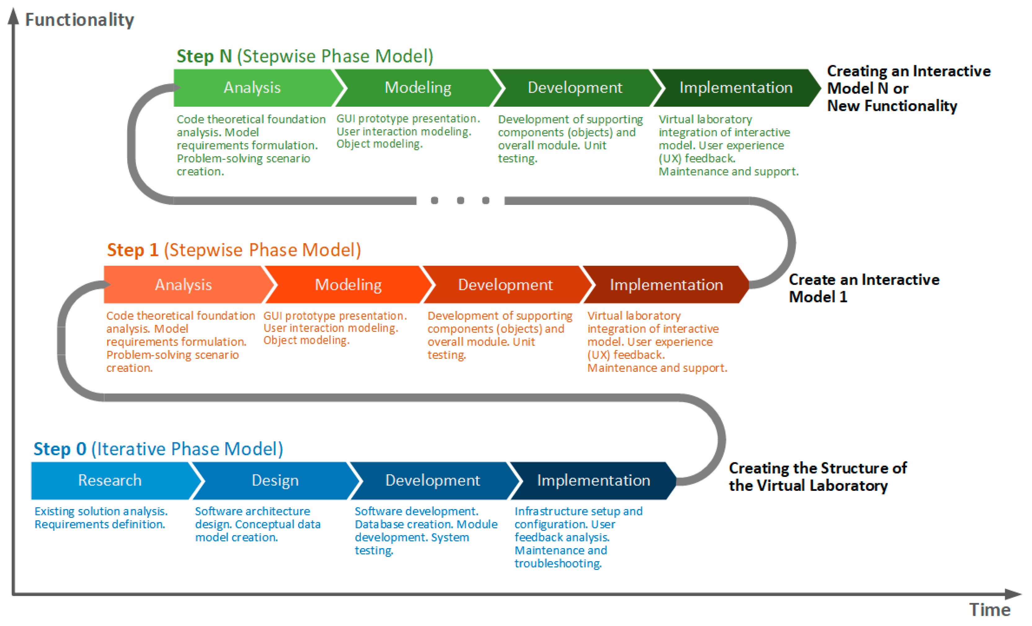
From the mentioned two varieties of the phase models, a variant is chosen in which both forms are applied for the development of the virtual laboratory. Figure 2 gives the general form of the proposed hybrid methodology. In the first step of the phase model, the structure (skeleton) of the web-based system with the corresponding pages is implemented, in which case the iterative variant of the phase model is more appropriate. In each subsequent step, the planned program models for solving tasks according to the relevant codes are designed and implemented, applying the step-by-step phase model.

2.2. Designing the Virtual Laboratory

  • Formulation of requirements for the virtual laboratory
    Well-thought-out and documented requirements for a software product are essential for its successful implementation. Requirements can be categorized into two groups: functional and non-functional. Functional requirements aim to define the desired behavior of the system through its functions, services, or what the system must perform. Through the non-functional requirements, the aim is to determine the quality of the software system through a set of standards used to assess the specific work, for example, speed, security, flexibility, etc. [26]
    o
    Functional requirements
    The following functional requirements are formulated for the virtual laboratory:
    • -
      The system interface should be in Bulgarian and English;
      -
      Logging into the system should be performed using a username and password;
      -
      The system should support two types of users—students and teachers;
      -
      Ability to control users—add, remove, change passwords, and manage groups for control work (tests);
      -
      Ability to control the conditions of the tasks;
      -
      Ability to include in its composition a set of interactive models for solving tasks for the following types of error control codes: Hamming code by general method—encoding mode and decoding mode; Hamming code by matrix method—encoding mode and decoding mode; Cyclic code by polynomial method—encoding mode; Cyclic code using linear feedback shift register—encoding mode.
      -
      For each solved task, the user receives incentive points according to previously specified criteria;
      -
      The system should support three modes for solving tasks:
      -
      “Training” mode (no set condition);
      -
      “Task” mode (solving a specific condition);
      -
      “Control work” mode (limited number of models launched).
      -
      The system should store information about the solved tasks, including data about the name of the software model used, including the mode of operation (encoding or decoding); time to solve the task; the number of mistakes made; the mistakes made; the number of points received from the task; and the condition of the task (only in “Control work” mode).
      -
      Obtaining reports from accumulated statistical data as follows: reference for the solved tasks of a specific user; reference for program models based on all tasks solved by users; report on the mistakes made when solving the tasks; ranking for the most active students.
    o
    Non-functional requirements
    The non-functional requirements for the virtual lab are as follows:
    • -
      The system should be platform-independent;
      -
      The system should be web-based and work with the most popular web browsers, such as Mozilla Firefox, Google Chrome, Microsoft Edge, Safari, etc.;
      -
      Data processing and system response should take minimal time;
      -
      Access to the system should be allowed only for registered users;
      -
      Access to the virtual laboratory should be possible at any time and from any place;
      -
      Not requiring the installation of additional software to work with the virtual laboratory;
      -
      The graphic interface of the administrative part and the interactive models should be intuitive and unified;
      -
      Data should be protected from illegal attacks.
  • Architecture of the virtual laboratory
    The general architecture of the designed virtual laboratory is given in Figure 3. It consists of four layers:
    o
    Presentation Layer. This layer represents the user interface through which users interact with the system. Its main purpose is to deliver information to and collect information from users. As can be seen from the architecture, the system is intended to support two types of users—students and teachers.
    o
    Business Logic Layer. It is the most important layer of the architecture and deals with the extraction, processing, transformation, and management of application data; enforcement of business rules and policies; and ensuring data consistency and validity. This layer consists of three main groups of modules:
    -
    Interactive models for solving tasks—this module includes the four planned software models: Hamming code by general and matrix method, cyclic code by polynomial method, and cyclic code by linear feedback shift register;
    -
    Modules for statistical reference—these modules summarize the accumulated data and provide information about the usability of the models for solving tasks, student activity, and the most active students and the mistakes made when solving the tasks;
    -
    Administrative modules—these modules serve to manage user profiles; manage assignment conditions and group students for control works.
    o
    Data Access Layer. Through this layer, a connection between the application and the data store (the database) is provided.
    o
    Data Layer. This layer takes care of storing the user profiles and the collected data from the work in the virtual laboratory.
The virtual laboratory does not provide material (presentations, documents) related to the subject area (coding theory), because these materials are published and available on the Ruse University e-learning platform (https://e-learning.uni-ruse.bg/index.php (accessed on 8 August 2024)) designed for asynchronous learning. It provides students with a manual for working with the individual interactive models in the form of video material.
The virtual laboratory includes separate (identical) software models for solving tasks in the field of coding theory. It is open and can be extended with various new interactive models from different subject areas, respecting the general requirements of the platform. The architecture of the virtual laboratory is designed to handle a large number of users, with performance largely dependent on server capacity.

3. Results

3.1. Implementation of a Coding Theory Virtual Laboratory

A web-based virtual lab has been created that offers an innovative learning environment for coding theory. The lab includes four interactive models designed to solve coding theory problems, allowing students to practice and refine their skills in real time. In addition, the platform has four statistical modules that provide valuable information about the usability of the models, student activity, analysis of errors made in solving the tasks, and ranking of the best students. To facilitate the administration of the laboratory, three administrative modules have been integrated that allow efficient management of user profiles, task conditions, and control work groups. These functionalities create a comprehensive and flexible learning platform that supports both educators and learners in the process of mastering complex coding theory concepts.
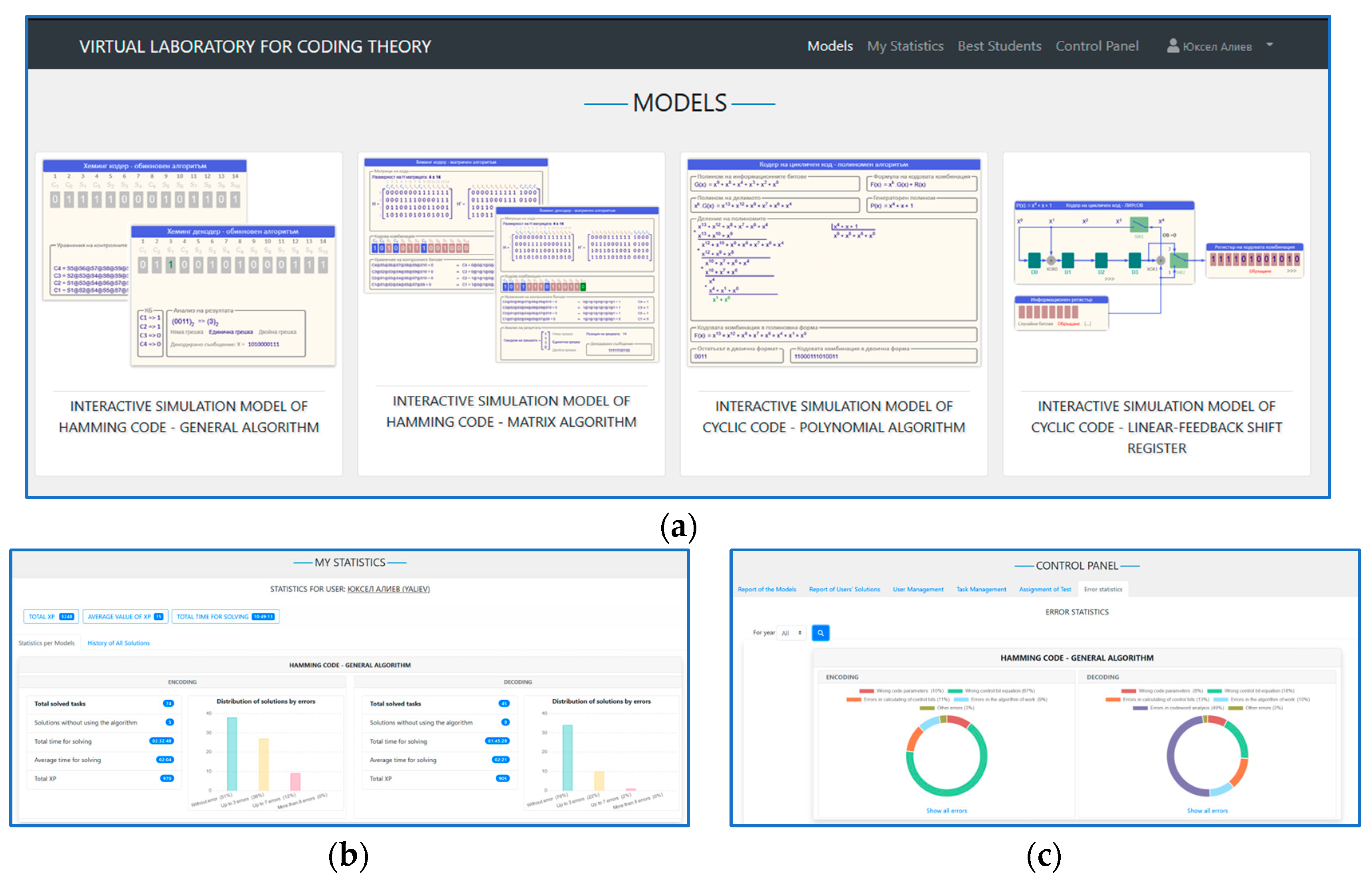
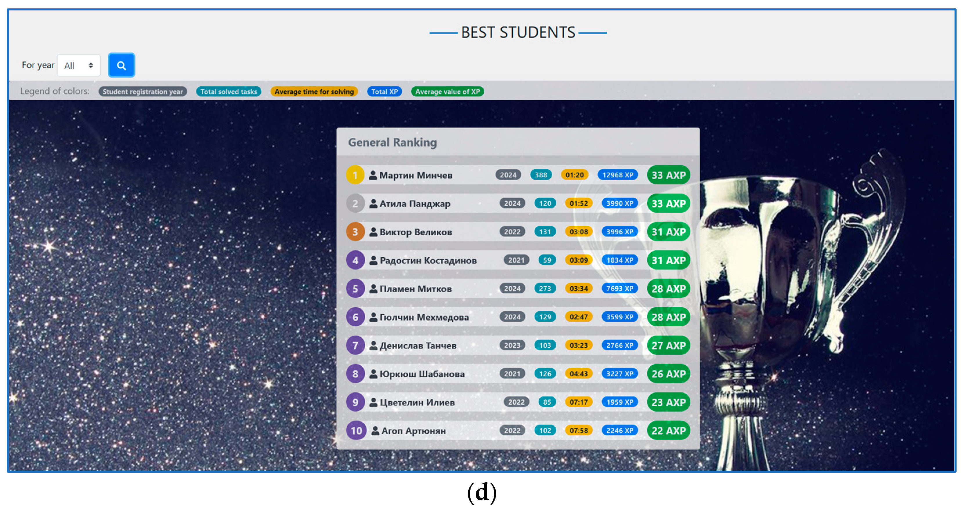
Figure 4a shows the page with the list of developed interactive models that the user can run and solve tasks. Figure 4b shows the page about the statistics of solved tasks, and Figure 4c shows the summary statistics of errors made when solving the tasks. Figure 4d shows the best students ranking page, with a total of 5 rankings available, one general and one for each interactive model.
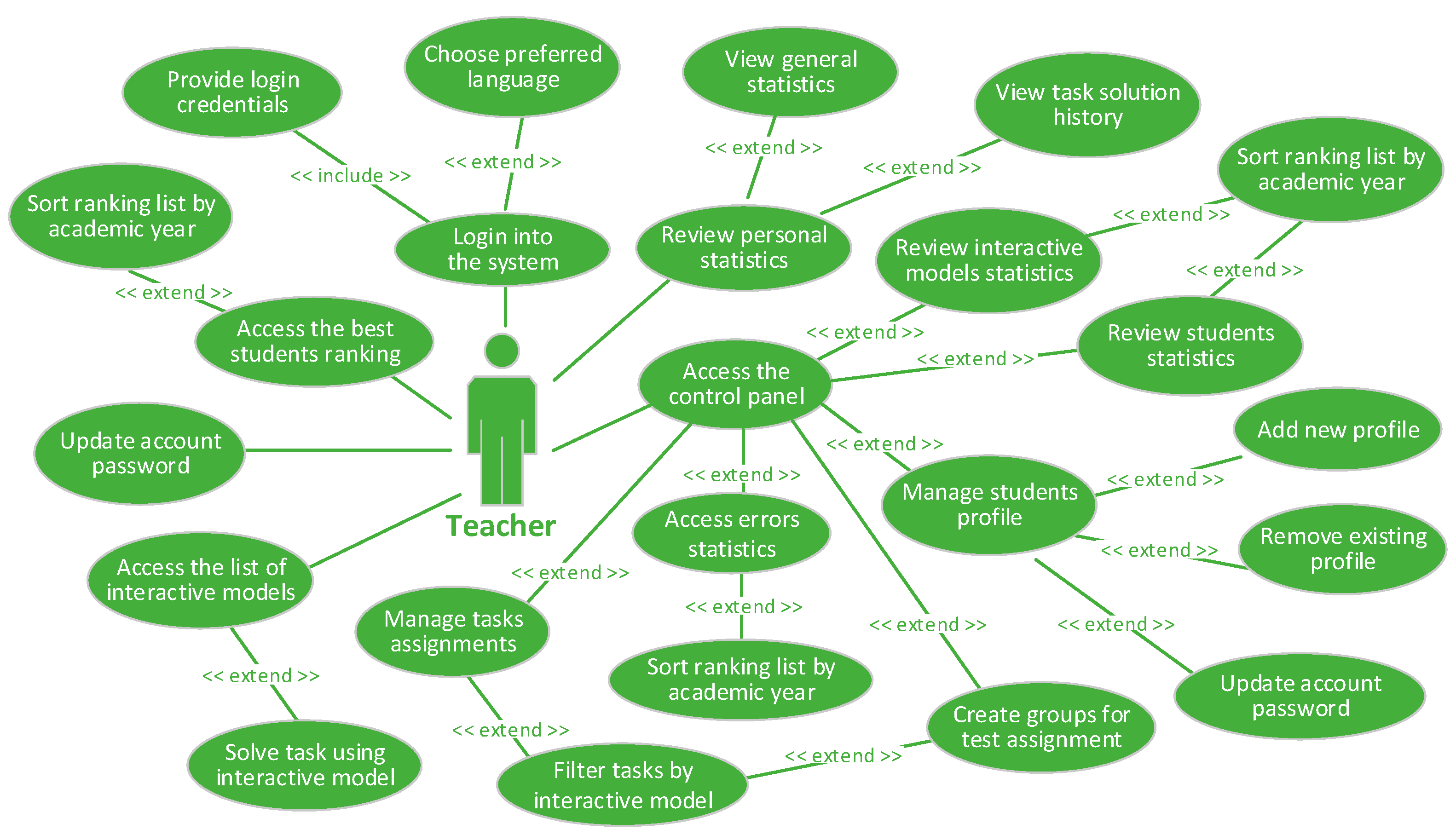
Figure 5 and Figure 6 illustrate the use-case diagrams of the virtual laboratory for students and teachers, respectively. Figure 5 presents the main actions that students can perform on the platform, including logging into the system, accessing the interactive models for solving coding theory problems, viewing their own results and errors, and participating in leaderboards (ranking of the best students). Figure 6 shows the use-case diagram for educators, which includes managing user profiles, setting assignment conditions, monitoring student activity, and generating statistical reports. These diagrams provide a visual overview of the functionalities available to the two main groups of users of the lab, highlighting the interactive and administrative capabilities of the platform.
The system was tested in a real learning process as the students sent their opinions, comments, remarks, and recommendations to improve the system. Based on the students’ feedback:
  • The interface design of individual interactive models was improved;
  • Errors (bugs) related to the operation of the interactive models were fixed;
  • Additional modules and functionalities were developed both for the entire virtual laboratory and for individual software models for studying the various codes.

3.2. Analysis of the Results of the Student Success Rate

The purpose of the analysis is to determine whether the use of a virtual laboratory has an impact on student achievement.
For the purpose of the experiment, two samples were formed. The first sample consists of students who studied the course “Reliability and Diagnostics of Computer Systems” (RDCS) from the specialty “Computer Systems and Technologies” at the University of Ruse “Angel Kanchev” in 2019 and 2020. The second sample is from students who studied the same course in 2021 and 2022. The first sample appears in the experiment as the “control group” and the second one as the “experimental group”. The difference between the two groups is that the students of the control group solved the tasks in a traditional way in written form (traditional methodology with paper and pen), when the virtual laboratory was not developed, and those of the experimental group—through the interactive software models from the virtual laboratory (experimental methodology). The main criterion for the selection of students from both groups is that they did not have poor grades (note: Poor 2 is the worst mark in Bulgaria, equivalent to “Failed”) in any subject in the previous two semesters, i.e., based on previous results. To compare the initial status of the two groups of students, the average grade from the previous two semesters (from all disciplines) was used, which was taken from the faculty office, and the grade from the current tests in the discipline, which was available from the teacher. It turned out that, according to this criterion, the number of students in the control group was initially greater than that in the experimental group, but it was subsequently decided by the teaching staff to equalize the number of students in the two groups to the lower number at random by the means of the statistical software used (SPSS version 26).
A total of 59 participants (including 51 males and 8 females) for the control group and 59 participants (including 53 males and 6 females) for the experimental group took part in the experiment. In recent years, in engineering majors (in particular, in the major “Computer Systems and Technologies”) in Bulgaria, mainly males are enrolled and the number of females is too small (there are graduates with only 1–2 females), which has given the authors reason not to analyze the results in terms of gender. The participants are between the ages of 20–27, studying in a 4-year full-time course, with the discipline being studied in the third year of their studies. No survey was carried out on their employment status.
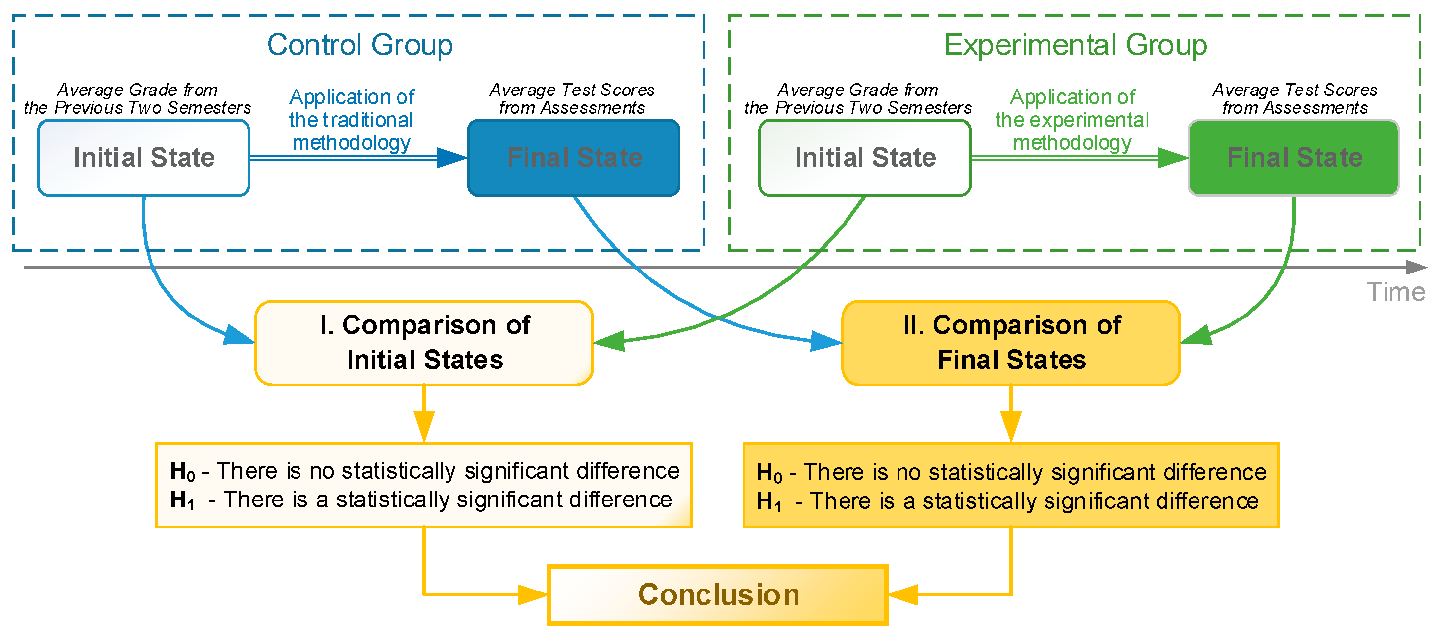
Figure 7 shows the structural scheme of the experiment, from which it is seen that the experiment consists of two comparisons—a comparison of the initial and final states of the students. The first comparison is made to find out whether there is a statistically significant difference in the average level of semester grades of the students between the two groups, i.e., whether students have an “equal start”. The second comparison aims to check whether there is a difference in the final state (average grade of the control works) between the two groups, i.e., “different ending”. As a result of the two comparisons, it should be established whether there is an impact from the use of the interactive software models.
The specialized software package Statistical Package for the Social Sciences [27] was used to carry out all the necessary operations of the experiment.

3.2.1. Statistical Hypothesis Checking of the Initial State of the Two Groups

At this point, it is checked whether there is a statistically significant difference in the average grade of the students from the control and experimental groups based on the average grade of the previous two semesters at the beginning of the experiment. The aim is to check whether the students were initially at approximately the same level before the influence of using the software models from the virtual laboratory.
  • Formulation of the hypotheses H0 and H1
    The following two hypotheses for the average grades are formulated:
    o
    Null hypothesis H 0 —There is no statistically significant difference;
    o
    Alternative hypothesis H 1 —There is a statistically significant difference.
  • Determination of the risk of error α
The risk of error or significance level (α) is the probability of rejecting the null hypothesis when it is true. It is set by the researcher and is usually referred to as the significance level. In practice, the risk of error is most often chosen to be α = 0.05 or α = 0.01 , which means that a risk of 5% or 1% is taken to reject the null hypothesis [28]. In this particular case, α = 0.05 is chosen as the risk of error.
  • Selection of criteria for checking the hypothesis
The parameter used to compare the two groups is the average grade of the previous two semesters. In order to make the comparison, the following steps must be taken:
  • o
    Determining whether the samples are dependent or independent
Since it is a question of students from control and experimental groups who studied the course in different years, two independent samples should be considered.
  • o
    Determining whether the criterion is parametric or non-parametric
The criterion is parametric when working with quantitative features and a normal distribution of the investigated feature. Accordingly, the criterion is non-parametric—for qualitative features and when the distribution of a quantitative feature does not follow a normal distribution or is unknown.
The mean score is a quantitative feature, but to determine whether to use a parametric criterion, a test for normality should be performed on the two groups separately.
  • o
    Checking for normal distribution by hypothesis testing
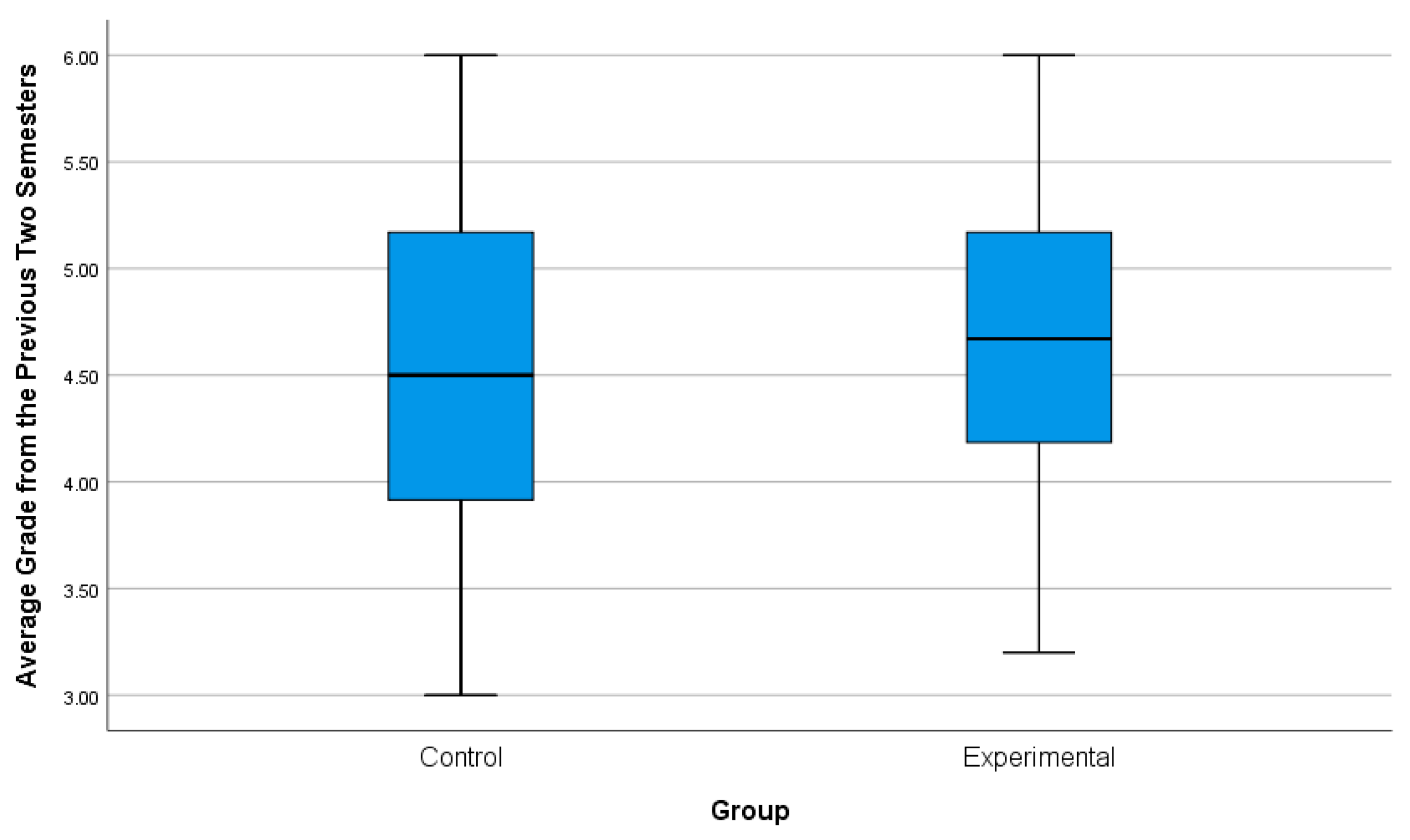
Before checking for a normal distribution of baseline mean scores for the two groups (in the initial states), it is important first to provide information about the general statistics of the data. It is also necessary to visualize the distribution of the data through a histogram that shows the frequency of the scores and a box-plot diagram that presents the distribution of the data, identifies potential deviations, and provides additional information about the symmetry and range of the scores. These steps provide a better understanding of the data before performing a more detailed statistical analysis. Figure 8 and Figure 9 show the histograms and box-plot diagrams of the groups, respectively. Descriptive statistics results for the two groups at the initial state are given in Table 1.
(1)
Formulation of the hypotheses for a normal distribution:
-
Null hypothesis H0—the variable has a normal distribution;
-
Alternative hypothesis H1—the variable does not follow a normal distribution.
(2)
Testing for normal distribution of the parameter for both groups.
There are many criteria (tests) for normal distribution, e.g., Lilliefors test, Kolmogorov–Smirnov test, Anderson–Darling test, etc. The Kolmogorov–Smirnov test is a non-parametric statistical test that is based on comparing the empirical cumulative distribution function (CDF) of a sample with that of a reference theoretical distribution. It measures the maximum difference between the two CDFs and is used to assess the similarity between different data sets or to check that they belong to the same theoretical distribution without requiring assumptions about the parameters of the distribution [29].
The results of the Kolmogorov–Smirnov test for a normal distribution of the average grades of students from the control and experimental groups are shown in Table 2 and Table 3, respectively. The most important result of the test is the so-called “asymptotic statistical significance”, which in the SPSS environment is marked with Asymp Sig. The decision criterion is as follows:
If α = 0.05 α s   ( A s y m p   S i g . ) , the distribution is not normal;
If α = 0.05 < α s   ( A s y m p   S i g . ) , the distribution is normal.
From the results thus obtained, it can be seen that for both groups the value of asymptotic statistical significance is α s = 0.200 . Since α = 0.05 < α s = 0.200 , the hypothesis H 0 should be accepted, i.e., the average grade of the control and experimental group students followed a normal distribution.
After it has been established that there is a normal distribution of the studied data, a parametric test for two independent samples should be conducted.
o
Parametric test for two independent samples
The empirical level of significance α s in SPSS is denoted by Sig., and the preset risk of error by α (the most often used value is 0.05).
A hypothesis test is performed about the difference between the means of the two independent samples. This check is undertaken by the Student’s parametric test (t-test). The conditions for using Student’s t-test for independent samples are as follows [30]:
  • -
    Application in null hypothesis testing;
    -
    The comparison parameter (average grade) is quantitative;
    -
    The comparison parameter has a normal distribution;
    -
    The two samples must be independent.
The current situation meets all these conditions. The decision criterion is as follows:
  • -
    If α α s , the hypothesis H0 is accepted (there is no statistically significant difference X c ¯ = X e ¯ );
    -
    If α   > α s , the hypothesis H1 is accepted (there is a statistically significant difference X c ¯   X e ¯ ).
The test results are given in Table 4.
  • Analysis of results
    -
    Checking for equality of variances
To ensure the validity of the t-test results, it is necessary to check for equality of variances of the two compared groups. This test can be performed using Levene’s Test, which is used to test the hypothesis of equality of variances of two or more samples. It is a statistical test that checks whether the sample variances are equal or not [31].
From Levene’s test (Table 4—the first part), it follows that the level of significance α s (denoted by Sig) is greater than the predetermined risk of significance α:
α s = 0.112   >   α = 0.05 ,
From which it follows that the means of the two groups have approximately equal variance.
  • -
    Test for statistically significant difference
Since the two groups have the same variances, the line equal variances assumed from Table 4 is considered. There it can be seen that for the level of significance Sig. 2-tailed it is obtained:
α s = 0.457   >   α = 0.05 .
After this check, the hypothesis H0 should be accepted, which states that there is no statistically significant difference between the two groups. This proves that there is an equal start of the control and experimental groups at the beginning of the experiment.
The analysis of the statistical test for difference in means can be extended by evaluating the so-called “effect size”. Determining the effect size allows one to assess the practical significance of how large or small the difference in mean success rates is between the two groups, not just whether the difference is statistically significant. One way to calculate effect size is through Cohen’s Coefficient (Cohen’s d), which is defined as follows [27,32]:
d = M 1 M 2 S D p o o l e d .
where
-
M 1 and M 2 are the mean values of average grades for the control and experimental groups, respectively, where M 1 = 4.5829 and M 2 = 4.6810 (Table 1).
-
S D p o o l e d is the average standard deviation of the two groups, which is calculated as follows:
S D p o o l e d = n 1 1 . S D 1 2 + n 2 1 . S D 2 2 n 1 + n 2 2 .
where
-
n 1 and n 2 are, respectively, the sizes of the samples, which in the specific case for both groups are n 1 = n 2 = 59 (Table 2 and Table 3);
-
S D 1 and S D 2 are the standard deviations for the control and experimental groups, respectively, where S D 1 = 0.77649 and S D 2 = 0.64586 (Table 1).
After substitution with the corresponding values S D p o o l e d is obtained:
S D p o o l e d = 0.71417
and Cohen’s d is obtained:
d = 0.13736
When calculating Cohen’s d, the value of d = 0.13736 means that there is a small difference between the two groups, with the “–” sign indicating that the mean of the control group is slightly lower than that of the experimental group. However, the effect value is quite small.

3.2.2. Statistical Testing of Hypotheses About the Final State of the Two Groups

The purpose of this investigation is to determine the impact of the virtual laboratory on student achievement. In the analysis of the results for the final state, an average evaluation of control works of the following three types of tasks will be used:
  • -
    Hamming code by general method;
    -
    Hamming code by matrix method;
    -
    Cyclic code by polynomial method.
  • Formulation of the hypotheses H0 and H1
    o
    Null hypothesis H 0 —There is no statistically significant difference;
    o
    Alternative hypothesis H 1 —There is a statistically significant difference.
  • Determination of the risk of error α
α = 0.05 is chosen for the risk of error.
  • Selection of criteria for testing the hypothesis
The parameter used to compare the two groups is the average grade from control works. To make the comparison, one must go through the same steps as when comparing the initial state.
  • o
    Determining whether the samples are dependent or independent
Since it is a question of students from control and experimental groups who studied the course in different years, two independent samples should be considered.
  • o
    Checking for normal distribution by hypothesis testing
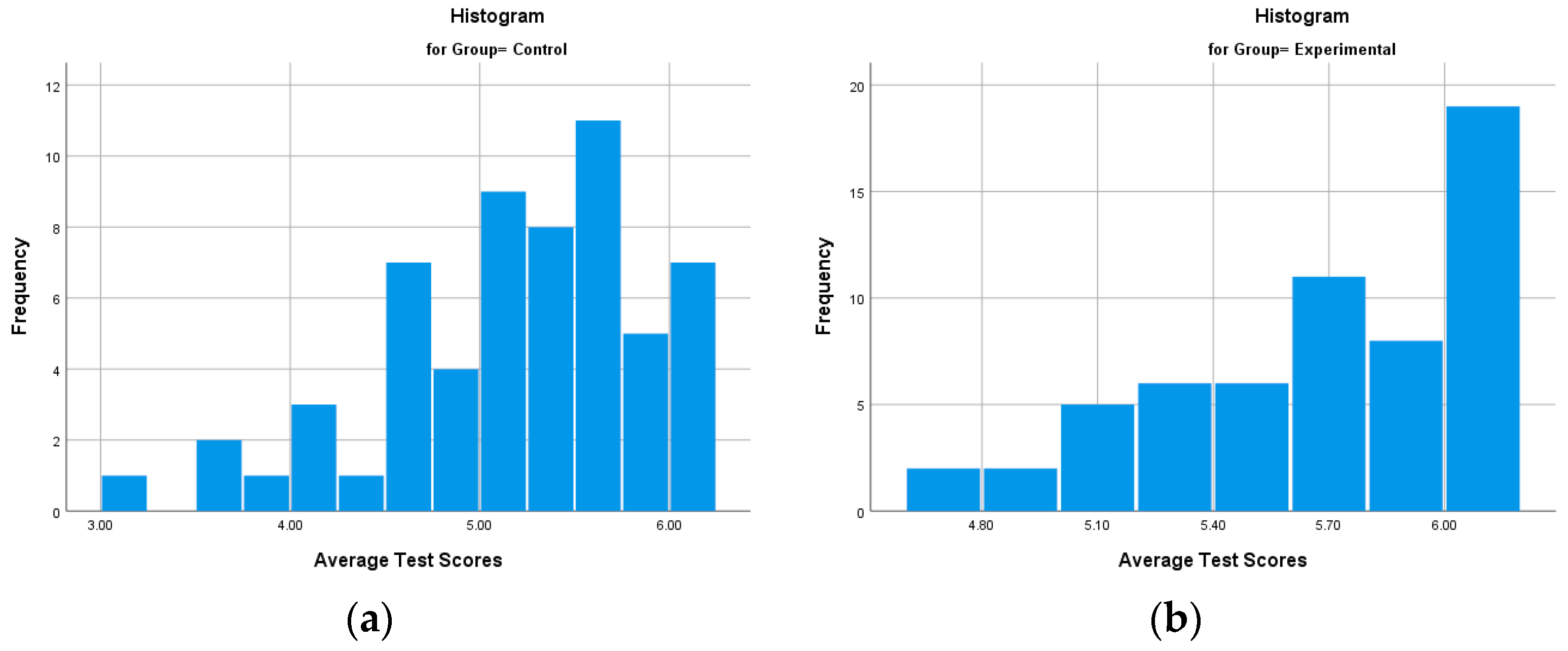
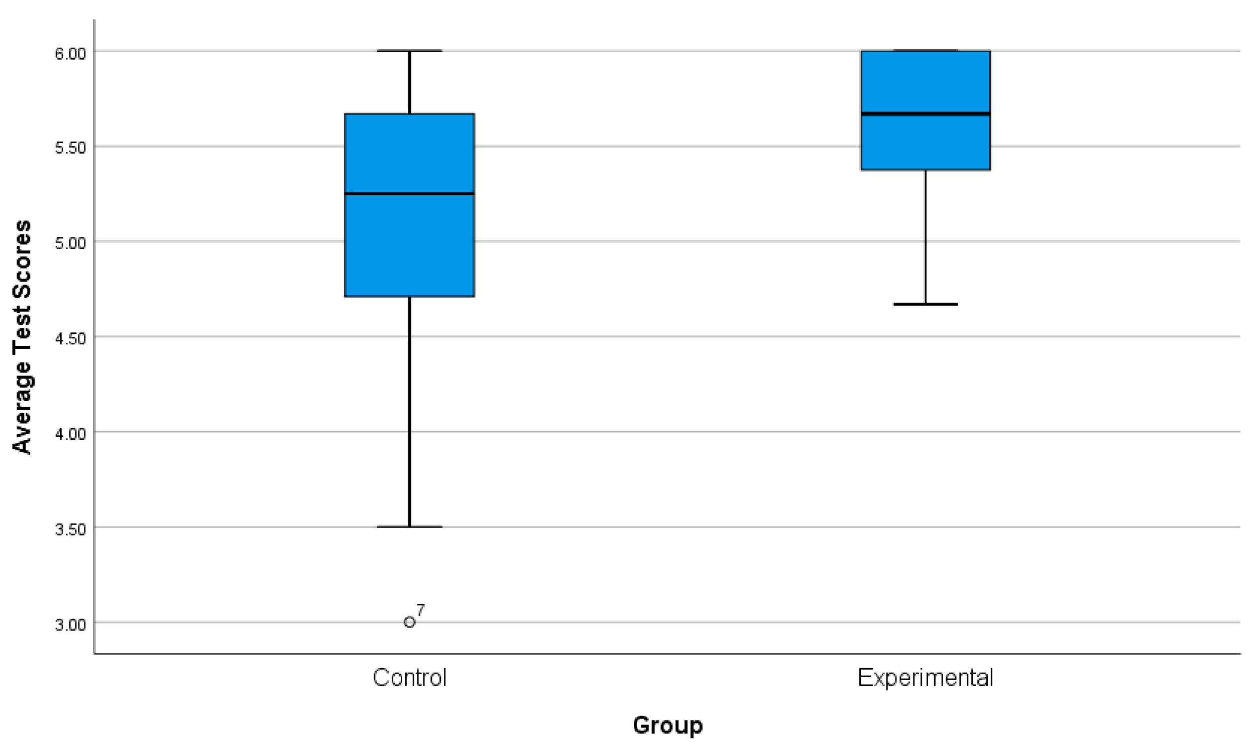
Before testing the normality of the data from the two samples, the summary statistics of the data should be presented, as was the case when comparing the initial state. Figure 10 and Figure 11 show the histograms and box-plot diagrams of the groups, respectively. Descriptive statistics results for the two groups at the final state are given in Table 5.
  • Checking for normal distribution by hypothesis testing
    (1)
    Formulation of the hypotheses for a normal distribution:
    -
    Null hypothesis H0—the variable has a normal distribution;
    -
    Alternative hypothesis H1—the variable does not follow a normal distribution.
    (2)
    Testing for normal distribution of the parameter for both groups.
The Kolmogorov–Smirnov test is again used to check for normal distribution. The results of the Kolmogorov–Smirnov test for the control and experimental groups are shown in Table 6 and Table 7, respectively.
According to the results of Table 6 and Table 7, for the distribution of data of the control and experimental group in the final state, the hypothesis H1 is accepted, i.e., the data do not follow a normal distribution because for the control group, α = 0.05 > α s = 0.012 , and for the experimental group, α = 0.05 > α s = 0.000 .
After it has been determined that both samples do not follow a normal distribution, a non-parametric test for two independent samples should be performed.
o
Non-parametric test for two independent samples
The decision criterion is as follows:
  • -
    If α α s , the hypothesis H0 is accepted (there is no statistically significant difference X c ¯ = X e ¯ );
    -
    If α   > α s , the hypothesis H1 is accepted (there is a statistically significant difference X c ¯   X e ¯ ).
This check is performed on a non-parametric basis using the Mann–Whitney test. The Mann–Whitney test is based on the ranks of the data. Ranks are assigned to the data, starting with the smallest and proceeding to the largest [18].
The test results are given in Table 8 and Table 9.
  • Analysis of the results
Comparing the value αs (Asymp. Sig. (2-tailed)) from Table 9 with the pre-set significance level α yields
αs = 0.000 < α = 0.05,
i.e., the hypothesis H1 is accepted, which states that there is a significant difference in mean scores (average grades), i.e., there was a statistically significant difference between the control and experimental groups at the end of the study.
Based on dependencies (3) and (4) for the final state, the following effect size results are obtained:
S D p o o l e d = 0.56070
d = 0.89691
In the final state, a value of d = 0.89691 was obtained, which means a significant difference between the two groups. A negative sign indicates that the difference is in the gain of the experimental group.

3.2.3. Conclusion of the Analysis

Key findings about the comparison between control and experimental groups are summarized in Table 10.
The mean rank from Table 8 of the experimental group is 72.86 and is higher than the mean rank of the control group, which is 46.14. Since the magnitude level of significance αs = 0.000 < α = 0.05, this ensures the statistical credibility of the conclusion that the success rate of the experimental group is actually higher than the success rate of the control group.
The absence of a statistically significant difference between the control and experimental groups at the beginning of the study (equal start) and the presence of a statistically significant difference between the control and experimental groups at the end of the study (different end) prove the following:
  • Effectiveness of the training method: the difference in average grades after the experiment shows that the web-based virtual laboratory had a positive impact on student achievements. Since the control of the initial conditions was equalized (no statistically significant difference before the beginning), it can be concluded that the training method itself was a key factor in improving the results of the experimental group.
  • Potential of technology in education: the success of the experimental group suggests that using virtual labs may be a more effective way to learn than the traditional written method. Virtual labs likely provide greater opportunities for interactivity, visualization, and hands-on experiences that enhance understanding and absorption of material.
  • Recommendation for implementation of new technologies: the results of the experiment support the idea that integrating web-based platforms into the learning process can be beneficial. Based on these data, expanded use of such technologies can be recommended to improve learning outcomes and student engagement.
  • Need for additional research: despite the positive result, it is useful to conduct further research to evaluate the long-term effect of the use of virtual laboratories, as well as to examine different areas of learning to find out whether this method works equally effectively in different subjects.
In summary, the experimental group using the web-based virtual laboratory achieved higher achievements, indicating that this learning method may have a significant advantage over the traditional written method.
When comparing test scores between the control and experimental groups, it would be beneficial for the study to consider potential confounding variables that could affect the results, such as variations in teaching methods, student motivation, or prior knowledge. Utilizing methods like ANCOVA (Analysis of Covariance) could assist in accounting for these confounders, but will be the subject of future research.

3.3. Analysis of Statistical Information on System Usability

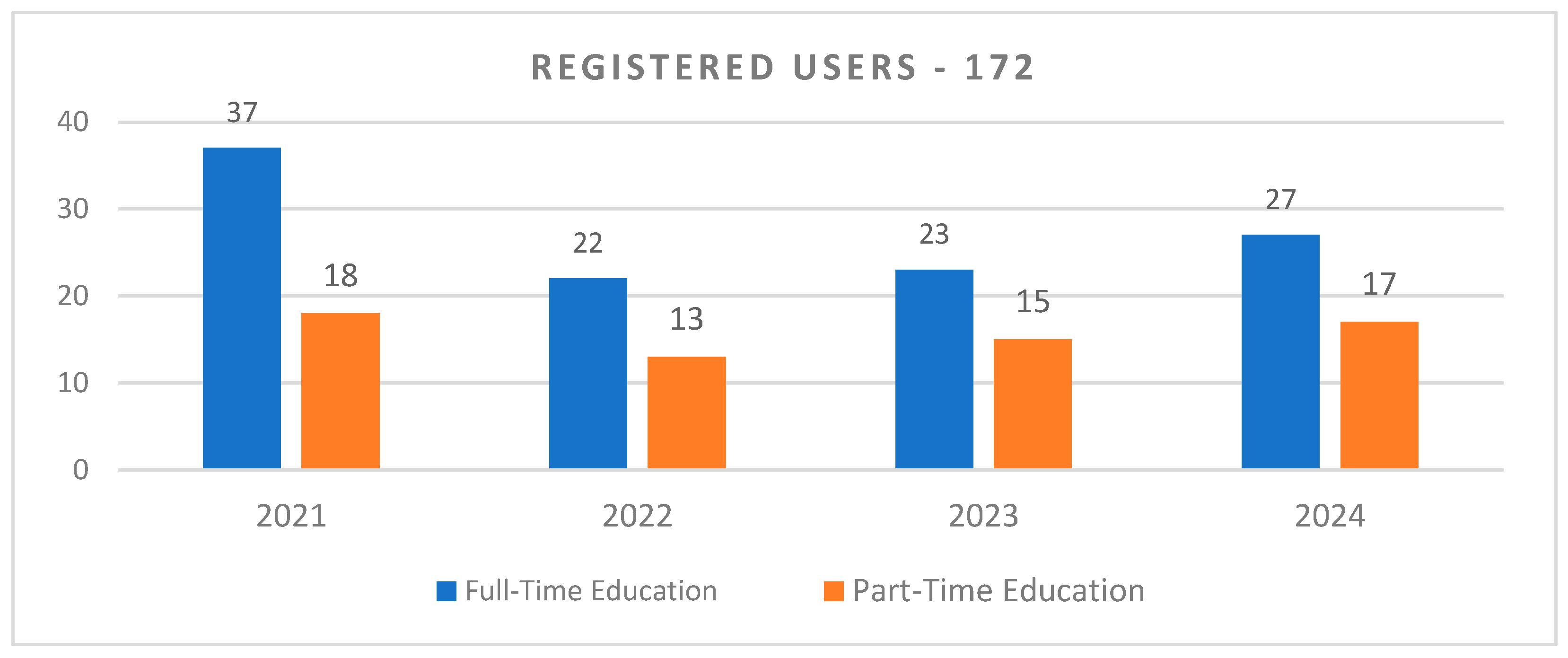
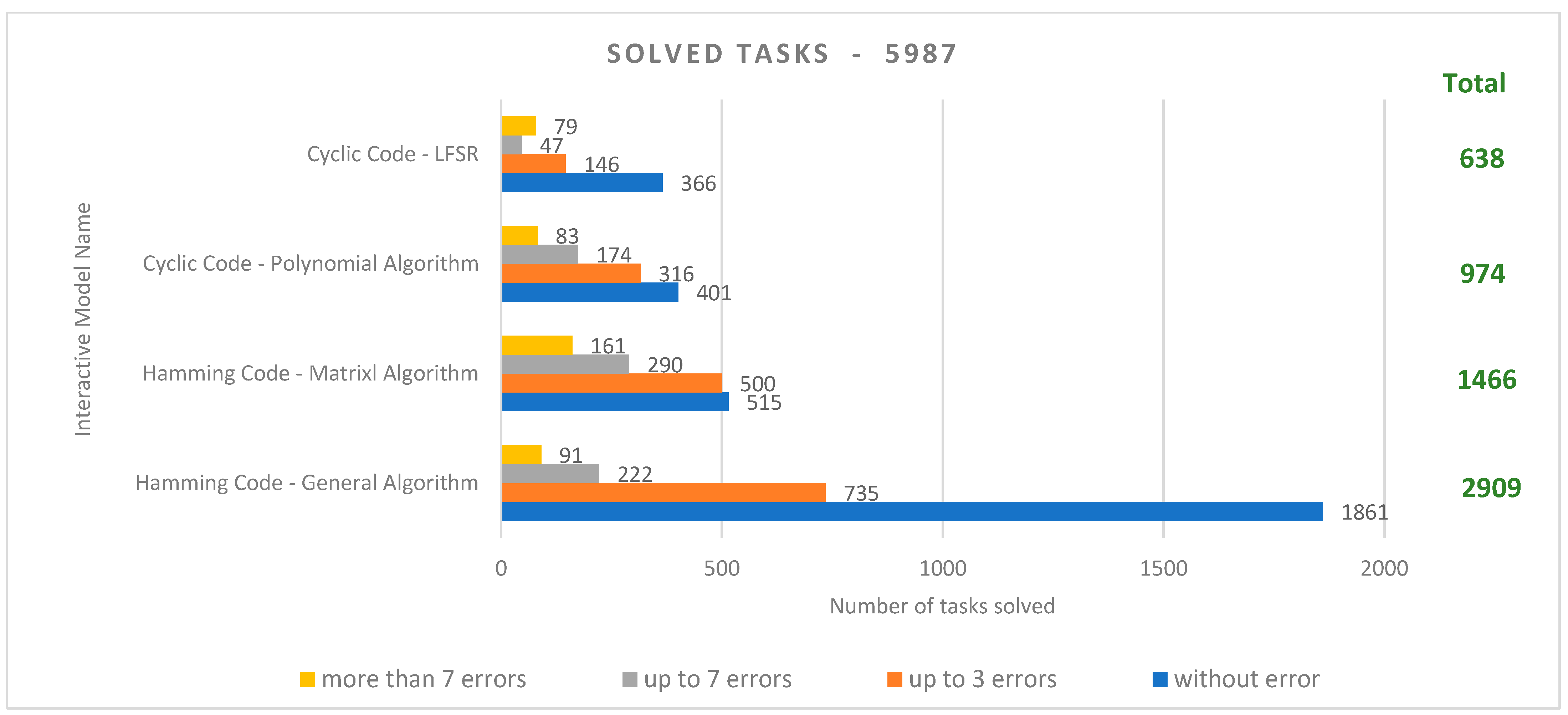
The virtual laboratory is used in the educational process from January 2021 to the present moment (2024). At the time of writing this article, the total number of registered student profiles is 128. Their distribution by years and form of education (full-time and part-time) is shown in Figure 12. Figure 13 shows the distribution of solved tasks with interactive models from the virtual laboratory.
The data from Figure 13 and Figure 14 about the number of registered 172 users in the virtual laboratory and the solved nearly 6000 tasks represent significant proof of the workability and high usability of the system. The data shows that over 50% of all solved problems were solved without an error or with up to three errors, which further emphasizes the effectiveness of the laboratory as a teaching tool. These results not only demonstrate the active participation of the students, but also validate the quality of the proposed tasks and the interactive models integrated in the laboratory. The total number of users and the tasks solved are strong indicators of the successful adoption and implementation of the virtual laboratory in the learning process.

3.4. Analysis of Data from a Survey on Students’ Opinions of the Use of the Virtual Laboratory

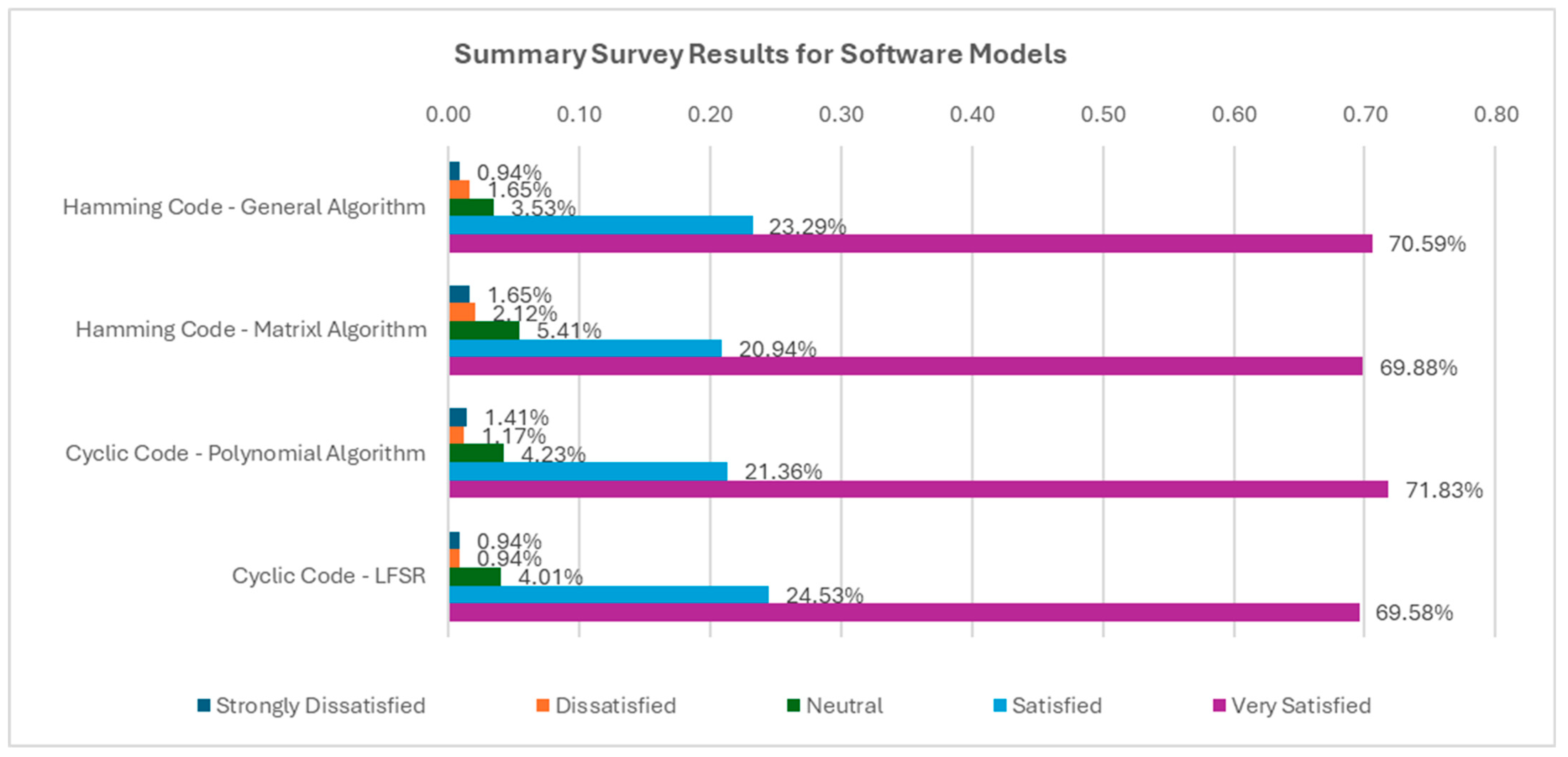
To study the opinion of the students regarding their satisfaction with the use of the interactive software models, a survey was conducted for the period from 2021–2023. The total number of students who participated in the surveys was 54. The survey was performed using Google Forms. Students rate their satisfaction with each interactive model according to various criteria on a five-point Likert scale as follows: “Strongly Dissatisfied”, “Dissatisfied”, “Neutral”, “Satisfied”, and “Very Satisfied”. The criteria by which the assessment is given cover various characteristics of the models, such as interface layout; easy orientation; website speed; problem-solving guide; description of the mathematical algorithm; practicing and strengthening problem-solving skills; statistics with the points for solved task and XP points for promotion.
The results of the survey are presented in Figure 14.
The results of the survey show a high degree of satisfaction with the use of the interactive software models. Analysis of the responses demonstrated that all four models received similar ratings from the respondents. The highest rating of “Very Satisfied” was indicated by approximately 70% of the participants, which highlights the positive perception of the models on all criteria, including interface, ease of orientation, and practical utility. The rating “Satisfied” was received by about 22% of the respondents, while “Neutral” was represented by about 4%. The negative ratings of “Strongly Dissatisfied” and “Dissatisfied” are kept to a minimum, not exceeding 3% in total, which clearly shows that the interactive models are effective and well accepted by students. These results once again confirm the successful integration of software tools into the learning process and their significant role in supporting coding theory learning.

4. Discussion

The created models facilitate the process of learning and consolidating students’ knowledge, thanks to their interactivity and timely feedback from checking the step-by-step solution of tasks.
The teachers involved in the design, implementation, and testing of the virtual laboratory in the educational process with students actively contributed their opinions and recommendations for improving the user interface and enhancing functionality, as well as addressing identified bugs in the software:
  • One of the main advantages recognized by the teachers is the software’s ability to automatically assign personalized tasks to each student. This feature significantly reduces the time required for teachers to prepare materials for exercises, tests, and course assignments.
  • A ranking system for the best active students was designed on the recommendation of the teachers, and this has led to a significant increase in the number of solved tasks completed by students. The ranking system has motivated students to solve more tasks, striving to minimize mistakes and improving their ranking.
  • Another requirement of the teaching staff was the automated identification of student mistakes and inserting the data for them in the database. This functionality has reduced the time teachers previously spent manually reviewing assignments before the virtual laboratory’s implementation. The review and grading process has been accelerated, facilitating the evaluation of a larger number of students in a shorter period.
  • Another important aspect, recommended by the teachers, is that the virtual laboratory ensures a transparent assessment process by automatically verifying results. This eliminates potential subjectivity in grading and guarantees that student evaluations are based on their actual achievements.
  • Furthermore, teachers report that the virtual laboratory is valuable for solving more complex tasks (with higher bit-rate information), which were difficult to achieve using traditional written methods.
A pedagogical experiment was conducted to determine the influence of interactive software models on student success. As a result of the research, it was found that the students who used the interactive software models to solve the tasks achieved better results compared to the students who worked in the traditional way (in written form).
The large number of solved tasks in the virtual laboratory allows us to conclude that maintaining different rankings of activity and achievements has a positive effect on students’ commitment to the learning process, stimulating them to solve more tasks as precisely as possible, striving to achieve better results in the ranking.
As a result of the survey conducted on student satisfaction with the interactive models included in the virtual laboratory, it was found that students give an overall positive assessment of the interface, orientation, speed of action, the guides provided, the descriptions of the algorithms, and the points awarded for a solved task and for encouragement and consider that working with the models helps to consolidate their knowledge, which is evidence of the usefulness of the virtual laboratory in learning coding theory.
It is necessary to investigate how the virtual laboratory can be integrated in different educational contexts and what its possibilities for mass application (scalability) are. In other words, it would be useful to consider how the virtual laboratory can be adapted and used in different educational settings (e.g., in different subjects, classes, universities, etc.) and to assess whether it can be expanded to serve a larger number of users or institutions.
The following points can be formulated:
  • Integration in different educational contexts: How the virtual laboratory can be used in different learning situations and environments (for example, in different educational systems or disciplines).
  • Scalability: Assessing the virtual lab’s potential to be implemented on a large scale, such as in many schools or universities simultaneously, and whether it can serve a large number of users.

Author Contributions

Conceptualization, A.B. and G.I.; formal analysis, Y.A., literature review Y.A.; investigation, G.I.; software, Y.A.; writing—original draft preparation, Y.A., A.B. and G.I.; writing—review and editing, Y.A., A.B., G.I.; visualization, Y.A.; implementation in a learning process, G.I.; funding acquisition, G.I.; data curation, G.I.; statistical data processing, Y.A.; project administration, G.I.; questionnaire survey, G.I. All authors have read and agreed to the published version of the manuscript.

Funding

This study is financed by the European Union-NextGenerationEU, through the National Recovery and Resilience Plan of the Republic of Bulgaria, project No. BG-RRP-2.013-0001-C01.

Institutional Review Board Statement

Not applicable.

Informed Consent Statement

Informed consent was obtained from all subjects involved in the study.

Data Availability Statement

All data used in the statistical study of this research can be accessed at the following address: https://ecsunirusebg-my.sharepoint.com/:f:/g/personal/yaliev_ecs_uni-ruse_bg/EpUJ2KKkGLhJhfsNObCl61EB3ajr9mckH46kDIZHQOdKZQ?e=nAQfjq (accessed on 2 September 2024).

Conflicts of Interest

The authors declare no conflicts of interest.

References

  1. Lewis, D.I. The Pedagogical Benefits and Pitfalls of Virtual Tools for Teaching and Learning Laboratory Practices in the Biological Sciences; The Higher Education Academy, STEM, 2014; Available online: https://citeseerx.ist.psu.edu/document?repid=rep1&type=pdf&doi=aa4c7290fbf0301cbbfc394f6085cd12692f5519 (accessed on 2 September 2024).
  2. Achuthan, K.; Francis, S.P.; Diwakar, S. Augmented reflective learning and knowledge retention perceived among students in classrooms involving virtual laboratories. Educ. Inf. Technol. 2017, 22, 2825–2855. [Google Scholar] [CrossRef]
  3. Achuthan, K.; Kolil, V.K.; Diwakar, S. Using virtual laboratories in chemistry classrooms as interactive tools towards modifying alternate conceptions in molecular symmetry. Educ. Inf. Technol. 2018, 23, 2499–2515. [Google Scholar] [CrossRef]
  4. Pastor, R. Online laboratories as a cloud service developed by students. In Proceedings of the IEEE Frontiers in Education Conference (FIE), Oklahoma City, OK, USA, 23–26 October 2013. [Google Scholar]
  5. Peidró, A.; Reinoso, O.; Gil, A.; Marín, J.M.; Payá, L. A virtual laboratory to simulate the control of parallel robots. IFAC-PapersOnLine 2015, 48, 19–24. [Google Scholar] [CrossRef]
  6. Valdez, M.; Ferreira, C.M.; Barbosa, F.P.M. 3D Virtual Laboratory for Teaching Circuit Theory—A Virtual Learning Environment (VLE). In Proceedings of the 51st International Universities’ Power Engineering Conference, Coimbra, Portugal, 6–9 September 2016. [Google Scholar] [CrossRef]
  7. Chao, J.; Chiu, J.L.; DeJaegher, C.J.; Pan, E.A. Sensor-augmented virtual labs: Using physical interactions with science simulations to promote understanding of gas behaviour. J. Sci. Educ. Technol. 2016, 25, 16–33. [Google Scholar] [CrossRef]
  8. Booth, C.; Cheluvappa, R.; Bellinson, Z.; Maguire, D.; Zimitat, C.; Abraham, J.; Eri, R. Empirical evaluation of a virtual laboratory approach to teach lactate dehydrogenase enzyme kinetics. Ann. Med. Surg. 2016, 8, 6–13. [Google Scholar] [CrossRef] [PubMed]
  9. Ahmad, A.; Nordin, M.K.; Saaid, M.F.; Johari, J.; Kassim, R.A.; Zakaria, Y. Remote control temperature chamber for virtual laboratory. In Proceedings of the IEEE 9th International Conference on Engineering Education (ICEED), Kanazawa, Japan, 9–10 November 2017; pp. 206–211. [Google Scholar]
  10. Erdem, M.B.; Kiraz, A.; Eski, H.; Çiftçi, Ö.; Kubat, C. A conceptual framework for cloud-based integration of Virtual laboratories as a multi-agent system approach. Comput. Ind. Eng. 2016, 102, 452–457. [Google Scholar] [CrossRef]
  11. Hashemipour, M.; Manesh, H.F.; Bal, M. A modular virtual reality system for engineering laboratory education. Comput. Appl. Eng. Educ. 2011, 19, 305–314. [Google Scholar] [CrossRef]
  12. Budai, T.; Kuczmann, M. Towards a modern, integrated virtual laboratory system. Acta Polytech. Hung. 2018, 15, 191–204. [Google Scholar] [CrossRef]
  13. Trnka, P.; Vrána, S.; Šulc, B. Comparison of Various Technologies Used in a Virtual Laboratory. IFAC-PapersOnLine 2016, 49, 144–149. [Google Scholar] [CrossRef]
  14. Ren, W.; Jin, N.; Wang, T. An Interdigital Conductance Sensor for Measuring Liquid Film Thickness in Inclined Gas-Liquid Two-Phase Flow. IEEE Trans. Instrum. Meas. 2024, 73, 9505809. [Google Scholar] [CrossRef]
  15. Okoyeigbo, O.; Agboje, E.; Omuabor, E.; Samson, U.A.; Orimogunje, A. Design and implementation of a java based virtual laboratory for data communication simulation. Int. J. Electr. Comput. Eng. (IJECE) 2020, 10, 5883–5890. [Google Scholar] [CrossRef]
  16. Erder, B.; Akar, A. Remote accessible laboratory for error controlled coding techniques with the labview software. Procedia-Soc. Behav. Sci. 2010, 2, 372–377. [Google Scholar] [CrossRef]
  17. Ersoy, M.; Kumral, C.D.; Çolak, R.; Armağan, H.; Yiğit, T. Development of a server-based integrated virtual laboratory for digital electronics. Comput. Appl. Eng. Educ. 2022, 30, 1307–1320. [Google Scholar] [CrossRef]
  18. Mertler, C.A. (Ed.) The Wiley Handbook of Action Research in Education; John Wiley & Sons: Hoboken, NJ, USA, 2019. [Google Scholar]
  19. Chatzopoulos, A.; Papoutsidakis, M.; Kalogiannakis, M.; Psycharis, S. Action Research Implementation in Developing an Open Source and Low Cost Robotic Platform for STEM Education. Int. J. Comput. Appl. 2019, 178, 33–46. [Google Scholar] [CrossRef]
  20. Chatzopoulos, A.; Kalogiannakis, M.; Papadakis, S.; Papoutsidakis, M. A novel, modular robot for educational robotics developed using action research evaluated on Technology Acceptance Model. Educ. Sci. 2022, 12, 274. [Google Scholar] [CrossRef]
  21. Dehalwar, K.; Sharma, S. Fundamentals of Research Writing and Uses of Research Methodologies; Edupedia Publications Pvt Ltd.: New Delhi, India, 2023. [Google Scholar] [CrossRef]
  22. Kapilan, N.; Vidhya, P.; Gao, X.Z. Virtual laboratory: A boon to the mechanical engineering education during COVID-19 pandemic. High. Educ. Future 2021, 8, 31–46. [Google Scholar] [CrossRef]
  23. Kemmis, S.; McTaggart, R.; Nixon, R. The Action Research Planner: Doing Critical Participatory Action Research; Springer: Singapore, 2014. [Google Scholar]
  24. Pressman, R.S. Software Engineering: A Practitioner’s Approach; McGraw-Hill: New York, NY, USA, 2010. [Google Scholar]
  25. Atkinson, C.; Weeks, D.C.; Noll, J. The design of evolutionary process modeling languages. In Proceedings of the 11th Asia-Pacific Software Engineering Conference, Busan, Republic of Korea, 30 November–3 December 2004; pp. 73–82. [Google Scholar] [CrossRef]
  26. Bell, E.; Thayer, T. Software requirements: Are they really a problem? In Proceedings of the 2nd International Conference on Software Engineering (ICSE), San Francisco, CA, USA, 13–15 October 1976; IEEE Computer Society Press: Washington, DC, USA, 1976; pp. 61–68. [Google Scholar]
  27. Field, A. Discovering Statistics Using IBM SPSS Statistics; Sage: Newcastle upon Tyne, UK, 2013. [Google Scholar]
  28. Mohammed, A.; Shayib, A. Applied Statistics, 1st ed.; Bookboon: London, UK, 2013; ISBN 978-87-403-0493-0. [Google Scholar]
  29. Stevens, J.P. Applied Multivariate Statistics for the Social Sciences, 5th ed.; Routledge: New York, NY, USA, 2012. [Google Scholar]
  30. Illowsky, B.; Dean, S. Introductory Statistics; Academic Press: Cambridge, MA, USA, 2013. [Google Scholar]
  31. Gray, C.D.; Kinnear, P.R. IBM SPSS Statistics 19 Made Simple; Psychology Press: Hove, UK, 2012. [Google Scholar]
  32. Durlak, J.A. How to select, calculate, and interpret effect sizes. J. Pediatr. Psychol. 2009, 34, 917–928. [Google Scholar] [CrossRef] [PubMed]
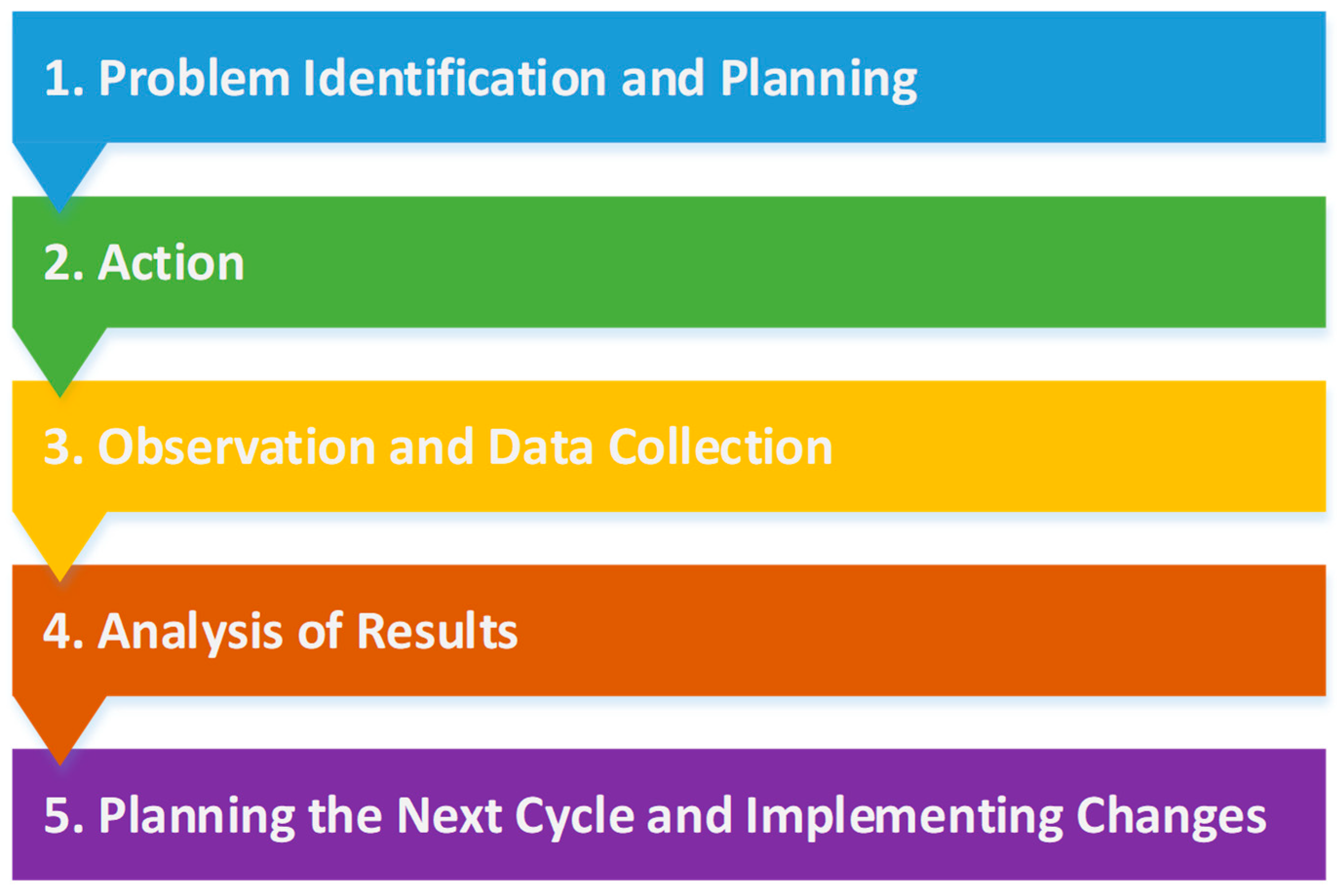
Figure 1. Research methodology.
Applsci 14 09546 g001
Figure 2. Methodology for design and development of the virtual lab.
Applsci 14 09546 g002
Figure 3. General architecture of the virtual laboratory.
Applsci 14 09546 g003
Figure 4. Screenshots of some components of the implemented virtual laboratory: (a) model list page; (b) statistics page for task solutions; (c) error statistics page; (d) best students ranking page.
Applsci 14 09546 g004aApplsci 14 09546 g004b
Figure 5. Student profile use-case diagram.
Applsci 14 09546 g005
Figure 6. Teacher profile use-case diagram.
Applsci 14 09546 g006
Figure 7. Structure of the experiment.
Applsci 14 09546 g007
Figure 8. Histogram of both groups at the initial state: (a) for the control group; (b) for the experimental group.
Applsci 14 09546 g008
Figure 9. Box-plot diagram of both groups at the initial state.
Applsci 14 09546 g009
Figure 10. Histograms of both groups at the final state: (a) for the control group; (b) for the experimental group.
Applsci 14 09546 g010
Figure 11. Box-plot diagram of both groups at the final state.
Applsci 14 09546 g011
Figure 12. Registered users in the virtual lab.
Applsci 14 09546 g012
Figure 13. Distribution of the solved tasks with the interactive models from the virtual laboratory.
Applsci 14 09546 g013
Figure 14. Average results of the survey on student satisfaction with the use of interactive models.
Applsci 14 09546 g014
Table 1. Descriptive statistics of both groups at the initial state.
Average Grade from the Previous Two Semesters
Group StatisticStd. Error
ControlMean4.58290.10109
95% Confidence Interval for MeanLower Bound4.3805
Upper Bound4.7852
5% Trimmed Mean4.5778
Median4.5000
Variance0.603
Std. Deviation0.77649
Minimum3.00
Maximum6.00
Range3.00
Interquartile Range1.34
Skewness0.2090.311
Kurtosis−0.8780.613
ExperimentalMean4.68100.08408
95% Confidence Interval for MeanLower Bound4.5127
Upper Bound4.8493
5% Trimmed Mean4.6699
Median4.6700
Variance0.417
Std. Deviation0.64586
Minimum3.20
Maximum6.00
Range2.80
Interquartile Range1.00
Skewness0.1310.311
Kurtosis−0.5540.613
Table 2. Results of the Kolmogorov–Smirnov test for the distribution of mean scores (average grades) for the control group at baseline (at the initial state).
One-Sample Kolmogorov–Smirnov Test a
Average Grade from the Previous Two Semesters
N59
Normal Parameters b,cMean4.5829
Std. Deviation0.77649
Most Extreme DifferencesAbsolute0.102
Positive0.102
Negative−0.072
Test Statistic0.102
Asymp. Sig. (2-tailed)0.200 d,e
a. Group = Control. b. Test distribution is normal. c. Calculated from data. d. Lilliefors Significance Correction. e. This is a lower bound of the true significance.
Table 3. Results of the Kolmogorov–Smirnov test for the distribution of mean scores (average grades) for the experimental group at baseline (at the initial state).
One-Sample Kolmogorov–Smirnov Test a
Average Grade from the Previous Two Semesters
N59
Normal Parameters b,cMean4.6810
Std. Deviation0.64586
Most Extreme DifferencesAbsolute0.096
Positive0.094
Negative−0.096
Test Statistic0.096
Asymp. Sig. (2-tailed)0.200 d,e
a. Group = Experimental. b. Test distribution is normal. c. Calculated from data. d. Lilliefors Significance Correction. e. This is a lower bound of the true significance.
Table 4. Results of the parametric test of the two independent samples at baseline (at the initial state).
Independent Samples Test
Levene’s Test for Equality of Variancest-Test for Equality of Means
FSig.tdfSig.
(2-Tailed)
Mean DifferenceStd. Error Difference95% Confidence Interval of the Difference
LowerUpper
Average Grade from the Previous Two SemestersEqual variances assumed2.5710.112−0.7461160.457−0.098140.13149−0.358570.16230
Equal variances not assumed −0.746112.2750.457−0.098140.13149−0.358660.16239
Table 5. Descriptive statistics of both groups at the final state.
Average Test Scores
Group StatisticStd. Error
ControlMean5.13710.09150
95% Confidence Interval for MeanLower Bound4.9540
Upper Bound5.3203
5% Trimmed Mean5.1865
Median5.2500
Variance0.494
Std. Deviation0.70284
Minimum3.00
Maximum6.00
Range3.00
Interquartile Range1.00
Skewness−0.8990.311
Kurtosis0.5090.613
ExperimentalMean5.64000.04780
95% Confidence Interval for MeanLower Bound5.5443
Upper Bound5.7357
5% Trimmed Mean5.6710
Median5.6700
Variance0.135
Std. Deviation0.36713
Minimum4.67
Maximum6.00
Range1.33
Interquartile Range0.67
Skewness−0.9620.311
Kurtosis0.2290.613
Table 6. Results of the Kolmogorov–Smirnov test for the distribution of mean scores (average grades) for the control group at the final state.
One-Sample Kolmogorov–Smirnov Test a
Average Test Scores
N59
Normal Parameters b,cMean5.1371
Std. Deviation0.70284
Most Extreme DifferencesAbsolute0.132
Positive0.110
Negative−0.132
Test Statistic0.132
Asymp. Sig. (2-tailed)0.012 d
a. Group = control. b. Test distribution is normal. c. Calculated from data. d. Lilliefors Significance Correction.
Table 7. Results of the Kolmogorov–Smirnov test for the distribution of mean scores (average grades) for the experimental group at the final state.
One-Sample Kolmogorov–Smirnov Test a
Average Test Scores
N59
Normal Parameters b,cMean5.6400
Std. Deviation0.36713
Most Extreme DifferencesAbsolute0.177
Positive0.163
Negative−0.177
Test Statistic0.177
Asymp. Sig. (2-tailed)0.000 d
a. Group = experimental. b. Test distribution is normal. c. Calculated from data. d. Lilliefors Significance Correction.
Table 8. Results of the Mann–Whitney rank test.
Ranks
GroupNMean RankSum of Ranks
Average Test ScoresControl5946.142722.00
Experimental5972.864299.00
Total118
Table 9. Statistical results of the non-parametric test.
Test Statistics a
Average Test Scores
Mann–Whitney U952.000
Wilcoxon W2722.000
Z−4.282
Asymp. Sig. (2-tailed)0.000
a. Grouping variable: group.
Table 10. Summary results of the pedagogical experiment.
Initial State ComparisonFinal State Comparison
Distribution of data
(Kolmogorov–Smirnov Test)
Control group—normal distribution;
Experimental group—normal distribution;
Control group—does not follow a normal distribution;
Experimental group—does not follow a normal distribution.
Test typeParametric test for two independent samples:
-t-test for equality of means;
-Levene’s test for equality of variances.
Non-parametric test for two independent samples:
Mann–Whitney rank test
Result (Hypothesis)H0: There is no statistically significant difference between the two groupsH1: There is a significant difference in mean scores (average grades)
Effect Sizes (Cohen′s d)Small effect (−0.137)Big effect (−0.897)
SummaryThere is an equal start for the control and experimental groups at the beginning of the experiment.The success rate of the experimental group is higher than the success rate of the control group at the end of the experiment.
Disclaimer/Publisher’s Note: The statements, opinions and data contained in all publications are solely those of the individual author(s) and contributor(s) and not of MDPI and/or the editor(s). MDPI and/or the editor(s) disclaim responsibility for any injury to people or property resulting from any ideas, methods, instructions or products referred to in the content.