
Prediction of Coiled Tubing Erosion Rate Based on Sparrow Search Algorithm Back-Propagation Neural Network Model


Abstract
1. Introduction
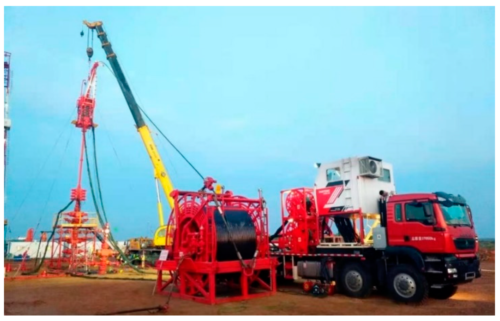
2. Experimental
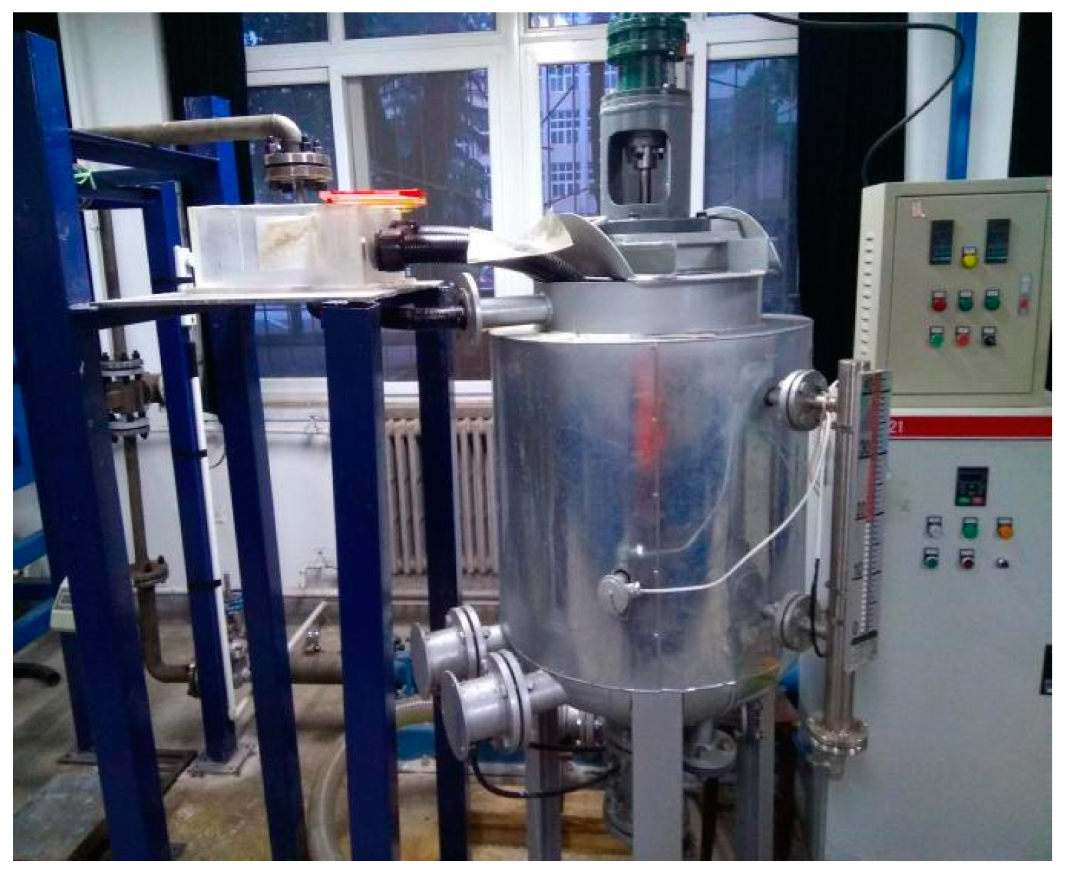
2.1. Experimental Device and Processes
- (1)
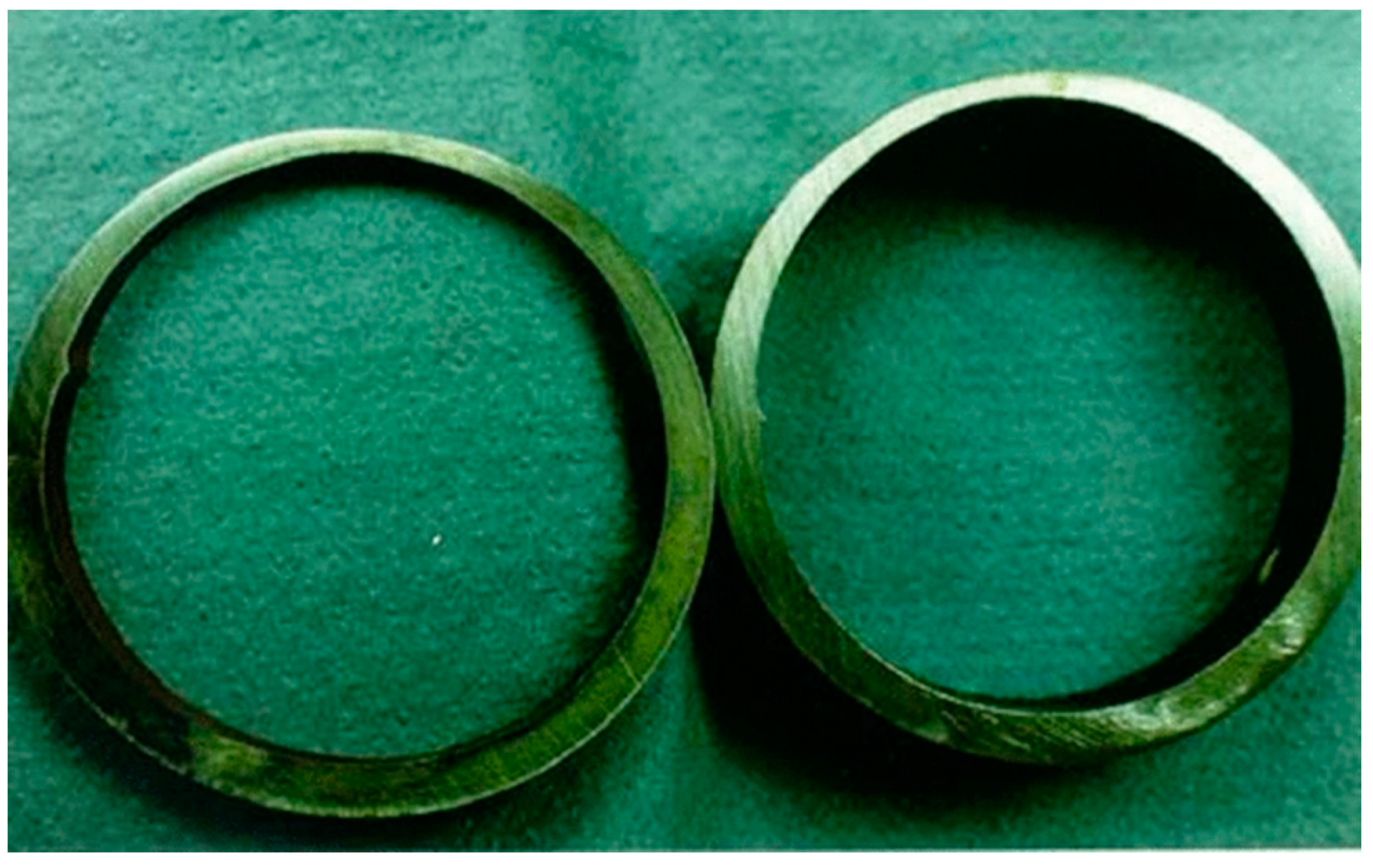
- Multiple sets of samples were cut from Φ50.8 mm × 4.4 mm coiled tubing with dimensions of 20 mm × 20 mm × 2 mm.
- (2)
- Unique identification numbers were assigned to the samples and they were weighed using a balance with a capacity of 100 g and an accuracy of 0.1 mg.
- (3)
- The samples were secured in the fixture and distance and angle were adjusted accordingly.
- (4)
- A 1 wt% KCl aqueous solution was poured into the sand-mixing barrel.
- (5)
- The mortar pump was started and the rotation speed was adjusted.
- (6)
- The 40–70 mesh silica sand was gradually added to achieve a sand concentration of 15–75 kg/m3.
- (7)
- The frequency converter was slowly adjusted to reach the predetermined impact velocity.
- (8)
- After the experiment was completed, the samples were removed, cleaned, and reweighed.
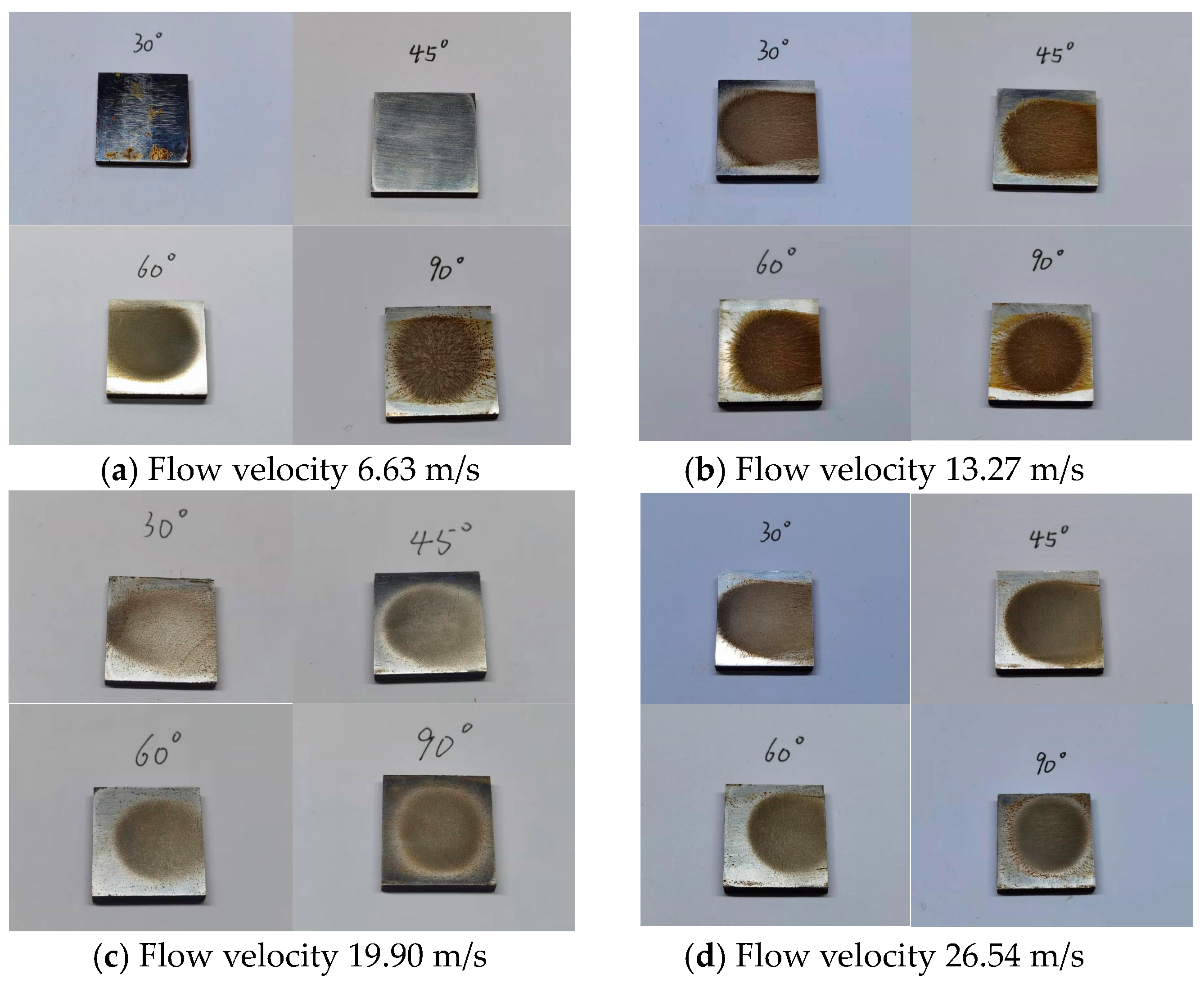
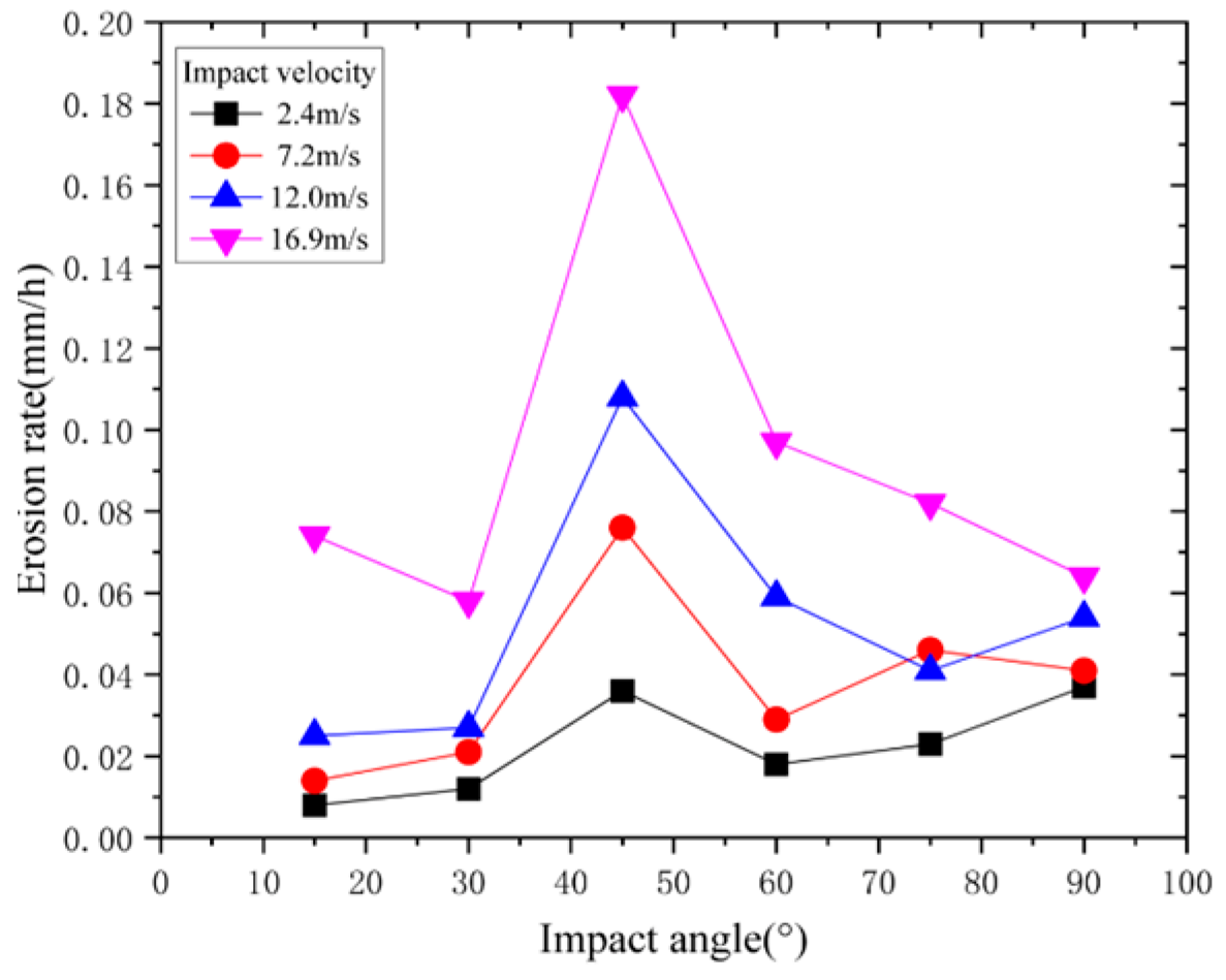
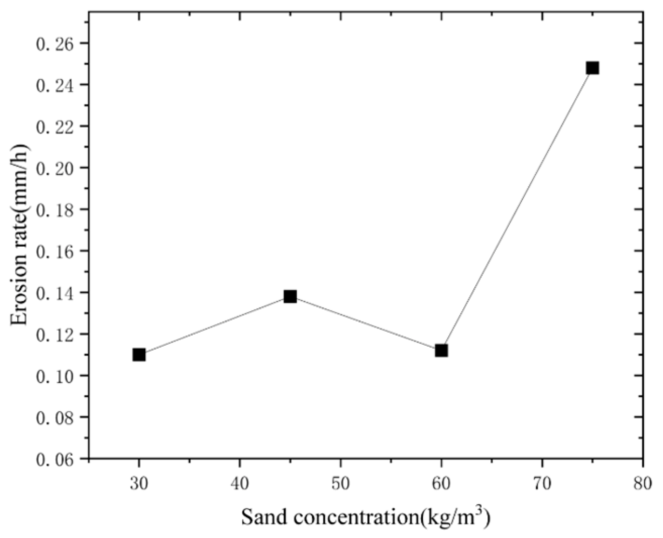
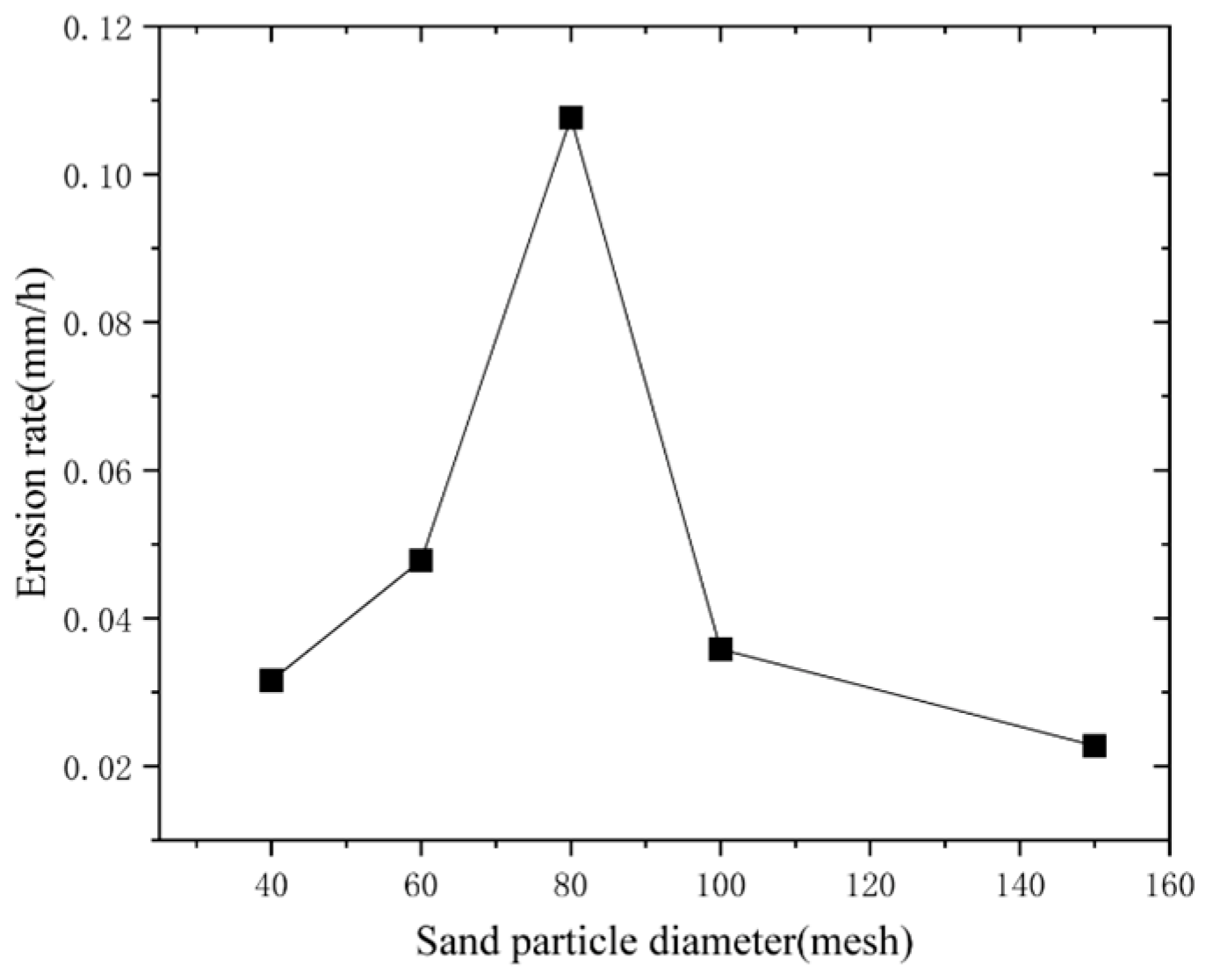
2.2. Experimental Results
3. GRA of Influencing Factors of Coiled Tubing Erosion Rate
- (1)
- Taking the erosion rate as the reference sequence, the impact angle, impact velocity, sand diameter, and sand concentration are used as the comparison sequence.
- (2)
- Perform dimensionless processing.
- (3)
- Calculate the relational coefficient between the comparison sequence xi and the reference sequence x0, as shown in Equation (1), where i is the index of features, i = 1, 2, ..., m, indicating different features; k is the index of samples, k = 1, 2, ..., n, representing distinct samples; [0, 1] is the resolution coefficient, usually 0.5.
- (4)
- Calculate the relational degree of the ith feature, as shown in Equation (2), where n denotes the total number of samples.
4. Methodology
4.1. Basic Principle of BPNN
4.2. Basic Principle of SSA
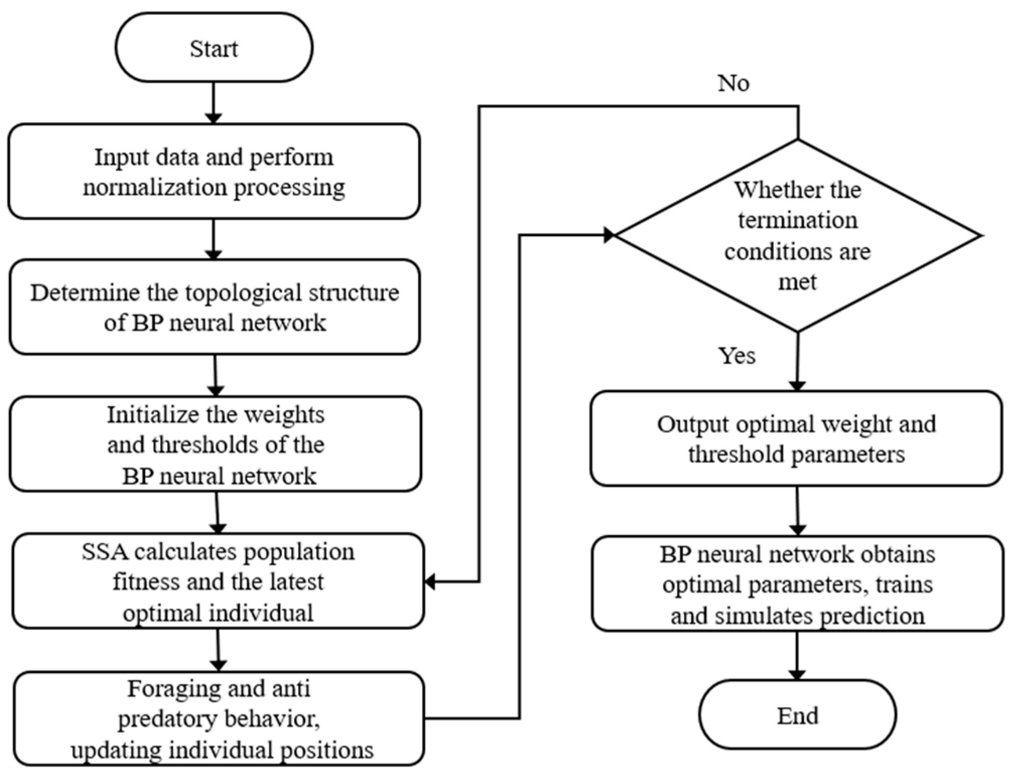
4.3. SSA-BPNN Model
- (1)
- Determine the structure of the BPNN according to the functional requirements.
- (2)
- The SSA is used to optimize the weight and threshold of the BPNN, and the initial optimal parameters are obtained.
- (3)
- The optimized optimal weights and thresholds are given to the BPNN to keep the network structure unchanged. Then, the optimized network is verified by experimental data.
5. Case Analysis
5.1. Data Selection
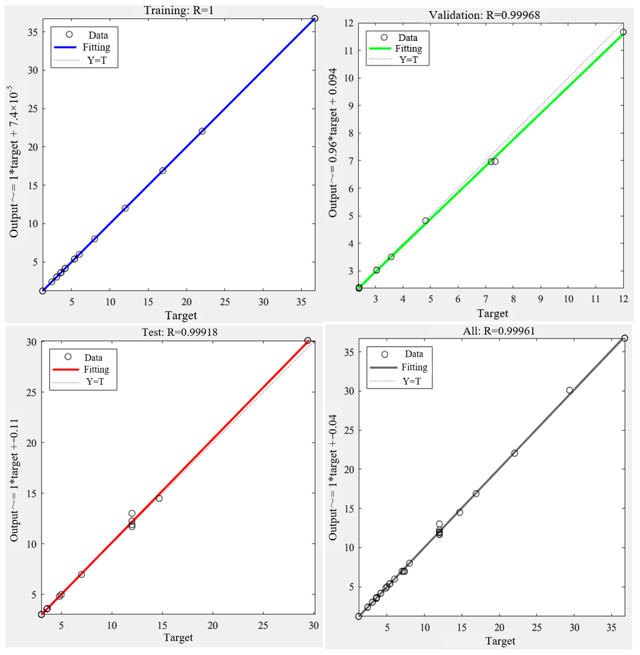
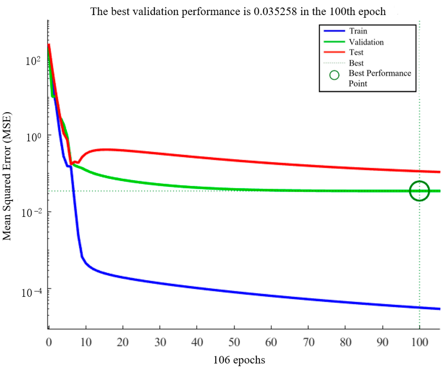
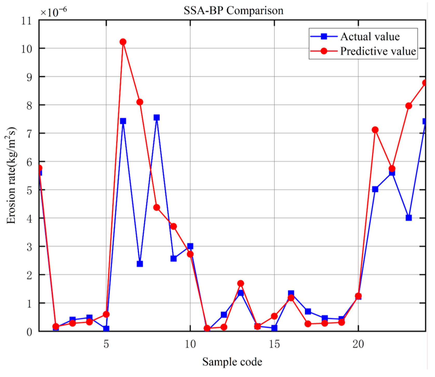
5.2. Results Analysis
6. Conclusions
- (1)
- Based on the experimental results, it is evident that the maximum erosion rate of the coiled tubing occurs at a 45° impact angle.
- (2)
- According to the GRA results, the impact velocity, impact angle, and sand concentration of the sand-carrying fluid have a strong influence on the erosion rate of coiled tubing, and the impact velocity has the greatest influence on the erosion rate of coiled tubing.
- (3)
- The SSA-BPNN model is reliable in predicting the erosion rate of coiled tubing, which can provide guidance for coiled tubing hydraulic sand blasting operation.
- (4)
- This method can provide a reference for the erosion rate of coiled tubing. In the future, influence factors such as the defect size and working conditions of coiled tubing can be considered.
- (5)
- The feature selection of the model is limited, because only five influencing parameters are selected as input parameters to predict the erosion rate of coiled tubing. This indicates that the influence of other parameters on the erosion rate may not be considered, which makes the model unable to fully explain the complexity of the erosion rate. In future model optimization, it is recommended to expand the scope of the dataset and consider a wider range of impact parameters.
Author Contributions
Funding
Institutional Review Board Statement
Informed Consent Statement
Data Availability Statement
Conflicts of Interest
References
- Jiang, G.C.; Li, Y.Z.; He, Y.B.; Dong, T.F.; Sheng, K.M.; Sun, Z. Subsection and Superposition Method for Reservoir Formation Damage Evaluation of Complex-Structure Wells. Pet. Sci. 2023, 20, 1843–1856. [Google Scholar] [CrossRef]
- Wang, Z.H.; Xu, Y.F.; Khan, N.; Zhu, C.L.; Gao, Y.H. Effects of the Surfactant, Polymer, and crude oil properties on the formation and stabilization of oil-based foam liquid films: Insights from the microscale. J. Mol. Liq. 2023, 373, 121194. [Google Scholar] [CrossRef]
- Xu, A.R.; Dou, Y.H.; Feng, C.X.; Zheng, J.; Cui, X.K. Coiled Tubing Erosion Prediction and Fracturing Fluid Parameters Optimization During Hydraulic Jet Fracturing. J. Fail. Anal. Prev. 2022, 22, 1276–1292. [Google Scholar] [CrossRef]
- Jia, P.; Zhu, X.X.; Xue, S.F.; Fang, J. Numerical Simulation on Coiled Tubing Erosion During Hydraulic Fracturing. J. Fail. Anal. Prev. 2020, 20, 1928–1938. [Google Scholar] [CrossRef]
- Cui, L.; Li, Z.; Dou, Y.H. Erosion–Corrosion Behavior of 20Cr Steel in Corrosive Solid–Liquid Two-Phase Flow Conditions. J. Fail. Anal. Prev. 2018, 18, 640–646. [Google Scholar] [CrossRef]
- Cheng, J.R.; Li, Z.; Zhang, N.S.; Dou, Y.H.; Cui, L. Experimental Study on Erosion-Corrosion of TP140 Casing Steel and 13Cr Tubing Steel in Gas–Solid and Liquid–Solid Jet Flows Containing 2 wt % NaCl. Materials 2019, 12, 358. [Google Scholar] [CrossRef]
- Zhou, H.; Ji, Q.F.; Liu, W.; Ma, H.Y.; Lei, Y.; Zhu, K.Q. Experimental Study on Erosion-Corrosion Behavior of Liquid–Solid Swirling Flow in Pipeline. Mater. Des. 2022, 214, 110376. [Google Scholar] [CrossRef]
- Xie, Z.Q.; Cao, X.W.; Li, Q.P.; Yao, H.Y.; Qin, R.; Sun, X. Experimental Study on Particle Movement and Erosion Behavior of the Elbow in Liquid-Solid Flow. Heliyon 2023, 9, e21275. [Google Scholar] [CrossRef]
- Beccati, N.; Ferrari, C.; Parma, M.; Semrrin, M. Euerian Multi-Phase CFD model for predicting the performance of a centrifugal dredge pump. Int. J. Comp. Meth. Exp. Meas. 2019, 7, 316–326. [Google Scholar]
- Marinack, M.C., Jr.; Mpagazehe, J.N.; Higgs, C.F., III. An Eulerian, lattice-based cellular automata approach for modeling multiphase flows. Powder Technol. 2012, 221, 47–56. [Google Scholar] [CrossRef]
- Sedrez, T.A.; Shirazi, S.A.; Rajkumar, Y.R.; Sambath, K.; Subramani, H.J. Experiments and CFD Simulations of Erosion of a 90° Elbow in Liquid-Dominated Liquid-Solid and Dispersed-Bubble-Solid Flows. Wear 2019, 426–427, 570–580. [Google Scholar] [CrossRef]
- Wang, G.; Gao, Q.F.; Kou, L.Y.; Zhang, P.; Wang, W.H.; Deng, J.F.; Zhu, X.J. Study on Liquid-Solid Jet Erosion Characteristics of 316L Stainless Steel. J. Mech. Sci. Technol. 2023, 37, 1871–1882. [Google Scholar] [CrossRef]
- Zhu, X.H.; Peng, P.; Jing, J.; Song, W. Research on Casing Erosion in Reservoir Section of Gas Storage Wells Based on Gas-Solid Two-Phase Flow. Eng. Fail. Anal. 2022, 142, 106688. [Google Scholar] [CrossRef]
- Bilal, F.S.; Sedrez, T.A.; Shirazi, S.A. Experimental and CFD Investigations of 45 and 90 Degrees Bends and Various Elbow Curvature Radii Effects on Solid Particle Erosion. Wear 2021, 476, 203646. [Google Scholar] [CrossRef]
- Liu, S.H.; Zhang, Y.W.; Tu, Y.L. Erosion Wear Law of Coiled Tubing Outer Wall. China Powder Sci. Technol. 2016, 22, 80–83. [Google Scholar]
- Cao, Y.P.; Chen, Z.T.; Dou, Y.H.; Zheng, J.; Kang, Z.F. Erosion Factor Analysis of Coiled Tubing with Helical Buckling. China Pet. Mach. 2023, 51, 143–148+156. [Google Scholar]
- Lai, F.; Wang, Y.; EI-Shahat, S.A.; Li, G.J.; Zhu, X.Y. Numerical Study of Solid Particle Erosion in a Centrifugal Pump for Liquid–Solid Flow. J. Fluid. Eng. 2019, 141, 121302. [Google Scholar] [CrossRef]
- Shah, S.N.; Jain, S. Coiled Tubing Erosion During Hydraulic Fracturing Slurry Flow. Wear 2008, 264, 279–290. [Google Scholar] [CrossRef]
- Zhao, X.Y.; Cao, X.W.; Xie, Z.Q.; Cao, H.G.; Wu, C.; Bian, J. Numerical Study on the Particle Erosion of Elbows Mounted in Series in the Gas-Solid Flow. J. Nat. Gas. Sci. Eng. 2022, 99, 104423. [Google Scholar] [CrossRef]
- Li, B.C.; Zeng, M.; Wang, Q.W. Numerical Simulation of Erosion Wear for Continuous Elbows in Different Directions. Energies 2022, 15, 1901. [Google Scholar] [CrossRef]
- Hong, B.Y.; Li, Y.B.; Li, X.P.; Ji, S.P.; Yu, Y.F. Numerical Simulation of Gas-Solid Two-Phase Erosion for Elbow and Tee Pipe in Gas Field. Energies 2021, 14, 6609. [Google Scholar] [CrossRef]
- Ahn, J.H.; Asif, R.; Lee, H.W.; Hwang, I.J.; Hu, J.W. Design and Material Optimization of Oil Plant Piping Structure for Mitigating Erosion Wear. Appl. Sci. 2024, 14, 5234. [Google Scholar] [CrossRef]
- Pandya, D.A.; Dennis, B.H.; Russell, R.D. A Computational Fluid Dynamics Based Artificial Neural Network Model to Predict Solid Particle Erosion. Wear 2017, 378–379, 198–210. [Google Scholar] [CrossRef]
- Shamshirband, S.; Malvandi, A.; Karimipour, A.; Goodarzi, M.; Afrand, M.; Petković, D.; Mahmoodian, N. Performance Investigation of Micro- and Nano-Sized Particle Erosion in a 90° Elbow Using an ANFIS Model. Powder Technol. 2015, 284, 336–343. [Google Scholar] [CrossRef]
- Deng, F.H.; Deng, Z.Q.; Liang, H.; Wang, L.H.; Hu, H.T.; Xu, Y. Life Prediction of Slotted Screen Based on Back-Propagation Neural Network. Eng. Fail. Anal. 2021, 119, 104909. [Google Scholar] [CrossRef]
- Wang, Q.; Sun, C.; Li, Y.L.; Liu, Y.C. Numerical Simulation of Erosion Characteristics and Residual Life Prediction of Defective Pipelines Based on Extreme Learning Machine. Energies 2022, 15, 3750. [Google Scholar] [CrossRef]
- Zangenehmadar, Z.; Moselhi, O. Assessment of Remaining Useful Life of Pipelines Using Different Artificial Neural Networks Models. J. Perform. Constr. Facil. 2016, 30, 04016032. [Google Scholar] [CrossRef]
- Shaik, N.B.; Pedapati, S.R.; Taqvi, S.A.A.; Othman, A.R.; Dzubir, F.A.A. A Feed-Forward Back Propagation Neural Network Approach to Predict the Life Condition of Crude Oil Pipeline. Processes 2020, 8, 661. [Google Scholar] [CrossRef]
- Shaik, N.B.; Pedapati, S.R.; Othman, A.R.; Bingi, K.; Dzubir, F.A.A. An Intelligent Model to Predict the Life Condition of Crude Oil Pipelines Using Artificial Neural Networks. Neural. Comput. Appl. 2021, 33, 14771–14792. [Google Scholar] [CrossRef]
- Macchini, R.; Bradley, M.S.A.; Deng, T. Influence of particle size, density, particle concentration on bend erosive wear in pneumatic conveyors. Wear 2013, 1–2, 21–29. [Google Scholar] [CrossRef]
- Huang, C.H.; Chang, H.Y.; Yang, C.H. A Novel Grey-Based Feature Ranking Method for Feature Subset Selection. J. Chin. Inst. Eng. 2021, 33, 14771–14792. [Google Scholar]
- Liao, K.X.; Yao, Q.K.; Wu, X.; Jia, W.L. A Numerical Corrosion Rate Prediction Method for Direct Assessment of Wet Gas Gathering Pipelines Internal Corrosion. Energies 2012, 5, 3892–3907. [Google Scholar] [CrossRef]
- Zhang, P.; Zhang, X.M.; Zhang, Y.M.; Zheng, Y.X.; Wang, T.Y. Gray Correlation Analysis of Factors Influencing Compressive Strength and Durability of Nano-SiO2 and PVA Fiber Reinforced Geopolymer Mortar. Nanotechnol. Rev. 2022, 11, 3195–3206. [Google Scholar] [CrossRef]
- Han, Y.L. Artificial Neural Network Technology as a Method to Evaluate the Fatigue Life of Weldments with Welding Defects. Int. J. Press. Vessels. Pip. 1995, 63, 205–209. [Google Scholar] [CrossRef]
- Nasiri, N.; Khosravani, M.R.; Weinberg, K. Fracture Mechanics and Mechanical Fault Detection by Artificial Intelligence Methods: A review. Eng. Fail. Anal. 2017, 81, 270–293. [Google Scholar] [CrossRef]
- Rumelhart, D.E.; Hinton, G.E.; Williams, R.J. Learning Representations by Back-Propagating Errors. Nature 1986, 323, 533–536. [Google Scholar] [CrossRef]
- Xue, J.K.; Shen, B. A Novel Swarm Intelligence Optimization Approach: Sparrow Search Algorithm. Syst. Sci. Control. Eng. 2020, 8, 22–34. [Google Scholar] [CrossRef]
- Hamey, L.G.C. XOR has No Local Minima: A Case Study in Neural Network Error Surface Analysis. Neural. Netw. 1998, 11, 669–681. [Google Scholar] [CrossRef]
- Nitta, T. Local Minima in Hierarchical Structures of Complex-Valued Neural Networks. Neural. Netw. 2013, 43, 1–7. [Google Scholar] [CrossRef]
- Cheng, J.R.; Yang, X.T.; Li, Z. Numerical simulation of Erosion for API Round Thread Connection in a Solid-liquid Two-phase Flow. China Pet. Mach. 2013, 34, 1067–1071. [Google Scholar]
- Cui, L.; Yang, Y.Q.; Li, J.W.; Li, M.F.; Chang, W.Q.; Cheng, J.R. Study on the Erosion Performance of QT1100 Coiled Tubing Steel in Liquid-Solid Two-phase Flow. China Pet. Mach. 2024, 10, 1–9. [Google Scholar]
- Vasić, M.V.; Jantunen, H.; Mijatović, N.; Nelo, M.; Velasco, P.M. Influence of coal ashes on fired clay brick quality: Random forest regression and artificial neural networks modeling. J. Clean. Product. 2023, 407, 137153. [Google Scholar] [CrossRef]


| Impact Velocity (m/s) | Impact Angle (°) | Weight Before (g) | Weight After (g) | Weight Loss (g) | Erosion Rate (mm/h) |
|---|---|---|---|---|---|
| 6.63 | 30 | 9.8391 | 9.8128 | 0.0263 | 0.042 |
| 6.63 | 45 | 9.7657 | 9.7165 | 0.0492 | 0.078 |
| 6.63 | 60 | 9.8689 | 9.8132 | 0.0557 | 0.089 |
| 6.63 | 90 | 9.8403 | 9.7979 | 0.0424 | 0.068 |
| 13.27 | 30 | 9.8521 | 9.8177 | 0.0344 | 0.055 |
| 13.27 | 45 | 9.8734 | 9.8208 | 0.0526 | 0.084 |
| 13.27 | 60 | 9.88 | 9.8185 | 0.0615 | 0.098 |
| 13.27 | 90 | 9.8573 | 9.8088 | 0.0485 | 0.077 |
| 19.90 | 30 | 9.8451 | 9.8008 | 0.0443 | 0.071 |
| 19.90 | 45 | 9.86 | 9.7976 | 0.0624 | 0.099 |
| 19.90 | 60 | 9.8485 | 9.8056 | 0.0429 | 0.068 |
| 19.90 | 90 | 9.841 | 9.7978 | 0.0432 | 0.069 |
| 26.54 | 30 | 9.7894 | 9.7101 | 0.0793 | 0.126 |
| 26.54 | 45 | 9.8898 | 9.8187 | 0.0711 | 0.113 |
| 26.54 | 60 | 9.8791 | 9.8137 | 0.0654 | 0.104 |
| 26.54 | 90 | 9.8601 | 9.8063 | 0.0538 | 0.086 |
| Rank of Relational Degree | Influencing Factor | Degree of Association |
|---|---|---|
| 1 | Impact velocity (15° impact angle) | 0.5975 |
| 2 | Impact velocity (30° impact angle) | 0.6420 |
| 3 | Impact velocity (45° impact angle) | 0.6290 |
| 4 | Impact velocity (60° impact angle) | 0.8124 |
| 5 | Impact velocity (75° impact angle) | 0.6465 |
| 6 | Impact velocity (90° impact angle) | 0.6989 |
| 7 | Impact angle (2.4 m/s impact velocity) | 0.6727 |
| 8 | Impact angle (7.2 m/s impact velocity) | 0.6336 |
| 9 | Impact angle (12 m/s impact velocity) | 0.7218 |
| 10 | Impact angle (16.9 m/s impact velocity) | 0.6839 |
| 11 | Sand concentration | 0.6636 |
| 12 | Sand particle diameter | 0.1827 |
| Parameter | Input Parameter Values |
|---|---|
| Number of nodes in the hidden layer | 3 |
| Transfer function | trainscg |
| Training method | SSA-BPNN |
| Maximum number of iterations | 1500 |
| Learning rate | 0.005 |
| Training convergence requirement | 10−4 |
| Sample Number | Input Parameters | Output Parameters | ||||
|---|---|---|---|---|---|---|
| Exhaust Volume (L/min) | Sand Ratio (%) | Impact velocity (m/s) | Sand diameter (mm) | Sand mass flow (kg/s) | Erosion rate (kg/(m2·s)) | |
| 1 | 100 | 10 | 1.21 | 0.1 | 0.3 | 5.27 × 10⁻⁸ |
| 2 | 200 | 10 | 2.41 | 0.1 | 0.598 | 1.47 × 10⁻⁷ |
| 3 | 250 | 10 | 3.04 | 0.1 | 0.755 | 4.17 × 10⁻⁷ |
| 4 | 300 | 10 | 3.62 | 0.1 | 0.894 | 4.44 × 10⁻⁷ |
| 5 | 350 | 10 | 4.17 | 0.1 | 1.035 | 5.66 × 10⁻⁷ |
| 6 | 400 | 10 | 4.82 | 0.1 | 1.197 | 9.21 × 10⁻⁷ |
| 7 | 450 | 10 | 5.4 | 0.1 | 1.341 | 1.21 × 10⁻⁶ |
| 8 | 250 | 5 | 3.04 | 0.1 | 0.587 | 1.14 × 10⁻⁷ |
| 9 | 300 | 5 | 3.62 | 0.1 | 0.399 | 1.33 × 10⁻⁷ |
| 10 | 250 | 10 | 3.04 | 0.1 | 0.755 | 4.17 × 10⁻⁷ |
| ··· | ··· | ··· | ··· | ··· | ··· | ··· |
| 55 | 300 | 10 | 3.57 | 0.7 | 4.5 | 7.43 × 10⁻⁶ |
| 56 | 300 | 10 | 3.57 | 0.9 | 4.5 | 8.05 × 10⁻⁶ |
| 57 | 300 | 10 | 3.57 | 0.3 | 4.5 | 5.63 × 10⁻⁶ |
| 58 | 300 | 15 | 3.57 | 0.3 | 6.75 | 8.44 × 10⁻⁶ |
| 59 | 300 | 20 | 3.57 | 0.3 | 9 | 1.21 × 10⁻⁵ |
| r2 | X2 | RMSE | MBE | MPE | Skew. | Kurt. | Mean Deviation | Standard Deviation | |
|---|---|---|---|---|---|---|---|---|---|
| SSA-BPNN | 0.998 | 1.76 | 1.25 × 10⁻⁶ | 5.83 × 10⁻⁷ | 0.1 | 1.648 | 4.971 | 0.056 | 1.25 |
Disclaimer/Publisher’s Note: The statements, opinions and data contained in all publications are solely those of the individual author(s) and contributor(s) and not of MDPI and/or the editor(s). MDPI and/or the editor(s) disclaim responsibility for any injury to people or property resulting from any ideas, methods, instructions or products referred to in the content. |
© 2024 by the authors. Licensee MDPI, Basel, Switzerland. This article is an open access article distributed under the terms and conditions of the Creative Commons Attribution (CC BY) license (https://creativecommons.org/licenses/by/4.0/).
Share and Cite
Cao, Y.; Fang, F.; Wang, G.; Zhu, W.; Hu, Y. Prediction of Coiled Tubing Erosion Rate Based on Sparrow Search Algorithm Back-Propagation Neural Network Model. Appl. Sci. 2024, 14, 9519. https://doi.org/10.3390/app14209519
Cao Y, Fang F, Wang G, Zhu W, Hu Y. Prediction of Coiled Tubing Erosion Rate Based on Sparrow Search Algorithm Back-Propagation Neural Network Model. Applied Sciences. 2024; 14(20):9519. https://doi.org/10.3390/app14209519
Chicago/Turabian StyleCao, Yinping, Fengying Fang, Guowei Wang, Wenyu Zhu, and Yijie Hu. 2024. "Prediction of Coiled Tubing Erosion Rate Based on Sparrow Search Algorithm Back-Propagation Neural Network Model" Applied Sciences 14, no. 20: 9519. https://doi.org/10.3390/app14209519
APA StyleCao, Y., Fang, F., Wang, G., Zhu, W., & Hu, Y. (2024). Prediction of Coiled Tubing Erosion Rate Based on Sparrow Search Algorithm Back-Propagation Neural Network Model. Applied Sciences, 14(20), 9519. https://doi.org/10.3390/app14209519