Research on Section Coal Pillar Deformation Prediction Based on Fiber Optic Sensing Monitoring and Machine Learning Algorithms

Abstract

The mining face under the close coal seam group is affected by the superposition of the concentrated stress of the overlying residual diagonally intersecting coal pillar and the mining stress, which can easily cause the instability and damage of the section coal pillars during the process of mining back to the downward face. Additionally, the traditional methods of monitoring such as numerical simulation, drilling peeping, and acoustic emission fail to realize the real-time and accurate deformation monitoring of the internal deformation of the section coal pillars. The introduction of the drill-hole-implanted fiber-optic grating monitoring method can realize real-time deformation monitoring for the whole area inside the coal pillar, which solves the short board problem of coal pillar deformation monitoring. However, fiber-optic monitoring is easily disturbed by the external environment, which is especially sensitive to the background noise of the complex underground mining environment. Therefore, taking the live chicken and rabbit well of Shaanxi Daliuta Coal Mine as the engineering background, the ensemble empirical modal decomposition (EEMD) is introduced for primary noise reduction and signal reconstruction by the threshold determination (DE) algorithm, and then the singular matrix decomposition (SVD) is introduced for secondary noise reduction. Finally, a machine learning algorithm is combined with the noise reduction algorithm for the prediction of the fiber grating strain signals of coal pillar in a zone, and DBO-LSTM-BP is constructed as the prediction model. The experimental results demonstrate that compared with the other two noise reduction prediction models, the SNR of the EEMD-DE-SVD-DBO-LSTM-BP model is improved by 0.8–2.3 dB on average, and the prediction accuracy is in the range of 88–99%, which realizes the over-advanced prediction of the deformation state of the coal column in the section.

1. Introduction

In the northern region of Shaanxi, many mines face the issue of close-distance coal seam group mining [1,2,3]. As a typical representative of shallow coal seam group mining, Daliuta Coal Mine [4] has numerous residual goaf coal pillars after mining, with the coal pillars and the roadway layout of the lower mining face arranged in an oblique crossing. Due to the influence of the oblique crossing angle of the overlying goaf residual coal pillars, the damage and deformation pattern of the section coal pillars during the mining of the underlying face are not well understood, posing uncertain safety risks to underground operations [5]. Therefore, it is crucial to clarify the deformation of section coal pillars under the influence of residual oblique coal pillars in the overlying goaf and to construct a prediction model for section coal pillar deformation using advanced technologies such as machine learning. This can help predict the deformation and damage state of section coal pillars during mining stages, enabling timely support measures and ensuring the real-time perception of coal pillar structure status and safe coal mine production [6].

Currently, monitoring the deformation of section coal pillars is an important part of underground face mining, and various monitoring methods have been extensively studied by scholars. Zhang [7] utilized the discrete element numerical simulation software FLAC3D 6.0-PFC 6.0 to establish a coupled model, meticulously studying the temporal and spatial processes of surrounding rock deformation and its deformation and failure characteristics, revealing the deformation and failure mechanisms of coal pillars and influencing factors. Bao [8] used similar simulation tests to study the deformation and failure mechanisms of overlying surrounding rocks and coal pillars in steeply inclined goafs. Shuli W. [9] employed the SOS microseism monitoring system to collect microseism events and data during the multi-seam mining process, revealing the spatiotemporal distribution and evolution patterns of microseism events, analyzing the differences and correlations of microseisms under high-position thick hard rock layers during multi-seam mining, and exploring the impact mechanism and differences of thick hard rock layers at high positions. Gong Shuang [10] observed the fracture forms and damage degrees of coal pillars through borehole peeping, finding that the crack formation rate in the charge section during deep hole blasting exceeds 85%, and, during shallow hole blasting, it exceeds 90%. Hongru Hao [11] analyzed the relationship between the Brillouin gain spectral characteristics and the inhomogeneity of strain distribution at different sampling points and proposed a new method to determine the fiber response length to improve the accuracy of embedded fiber displacement monitoring. Vlastimil Kajzar [12] monitored the deformation of the coal pillar and the displacement of the roof plate by means of 3D laser technology, and all the scans corresponded well with the results of elongation measurements and other measuring instruments. These studies, although making progress in monitoring the internal fracture forms of coal pillars, stress distribution in return airways, microseism monitoring of coal pillar areas, numerical simulation, and similar simulation tests, still face limitations in long-term monitoring and under the influence of complex underground conditions. Therefore, it is necessary to introduce monitoring methods that adapt to the complex underground mining conditions of coal mines and monitor the internal stress–strain characteristics of coal pillars.

To address these issues, current fiber-optic sensing technology has achieved long-distance real-time monitoring, overcoming the complex and variable on-site underground environment and discontinuous monitoring problems [13,14,15]. However, this technology has not yet been applied to monitor the internal deformation of section coal pillars. In the field of coal mine safety, there has been considerable research on deformation monitoring using fiber-optic sensing. Moffat [16] proposed a fiber-optic-based PVC pipe strain monitoring system, installing the proposed sensor in mine tunnels to monitor rock mass movement. Yugay [17] used fiber-optic sensors on mine support elements to monitor pressure changes on the support, equipped with visual displays for monitoring results, and conducted emergency predictions based on these results. Yurchenko et al. [18] proposed a fiber-optic sensor model for monitoring the stress of mine working machinery, ensuring a new generation of computer-aided measurement for underground mining. Hu Yanbo [19] introduced fiber-optic sensing technology to monitor the deformation of roadway surrounding rock, timely grasping the internal deformation characteristics of deep roadway surrounding rock and providing a scientific basis for stability control decisions of deep roadway surrounding rock. Chai J et al. [20] proposed a fiber-optic sensing-based method for partitioning voids in mining overlying rock mass, and combined with physical model tests, systematically investigated the size, distribution, and deformation characteristics of rock-mass voids, concluding that the rate of void expansion is affected by the change of stress and that stress regulation is a key factor in preventing void expansion and rock mass destabilization. Piao C et al. [21] studied the stress distribution law and motion characteristics of the strata under reamer pillar mining by physical similarity simulation experiments using distributed fiber-optic sensing technology and concluded that the deformation of the coal pillar would go through three stages under the safety critical state. Hu Y et al. [22] used the Brillouin light time-domain reflection method for dynamic deep coal seam mine floor mining damage and concluded that the accuracy of this method is improved by 7~10% compared with the traditional monitoring method.

Simultaneously, fiber-optic grating monitoring encounters certain noise redundancy issues, and accurate deformation data prediction is crucial for safe underground mining [23,24]. Therefore, it is essential to select suitable and efficient noise reduction algorithms to filter and reduce noise from the monitored signals, thereby improving the accuracy of data prediction. Common noise reduction methods include f-x domain predictive filtering [25], wavelet transform [26], data denoising methods based on empirical mode decomposition (EMD) [27], and ensemble empirical mode decomposition (EEMD) [28,29,30,31,32]. These studies have explored denoising decomposition algorithms in terms of the modal aliasing, decomposition completeness, and signal distortion of the IMF components after algorithm decomposition. However, there is a lack of appropriate threshold selection for the decomposed IMF components.

In summary, based on the deformation of section coal pillars in the Huojitu District of Daliuta Coal Mine, as the engineering background, this study uses fiber-optic grating sensing technology for real-time monitoring. It introduces the distribution entropy (DE) [33] combined with EEMD to construct a denoising algorithm model. The DE algorithm is used to filter the effective IMF components from the EEMD decomposed IMF components, eliminating the components with a high noise ratio, and reconstructing a signal with high fidelity. Subsequently, singular value decomposition (SVD) is employed for secondary noise reduction, laying the groundwork for subsequent optical fiber grating sensing prediction studies of section coal pillar deformation. This study aims to optimize the long short-term memory neural network with the dung beetle optimization (DBO) algorithm to construct a deformation prediction model for section coal pillars. It aims to achieve the real-time monitoring and prediction of section coal pillar deformation under shallow-buried close-distance residual oblique coal pillars, improving the safety factor of underground face mining, and providing guidance for roadway support and decision-making.

2. Background Overview

2.1. Work Conditions

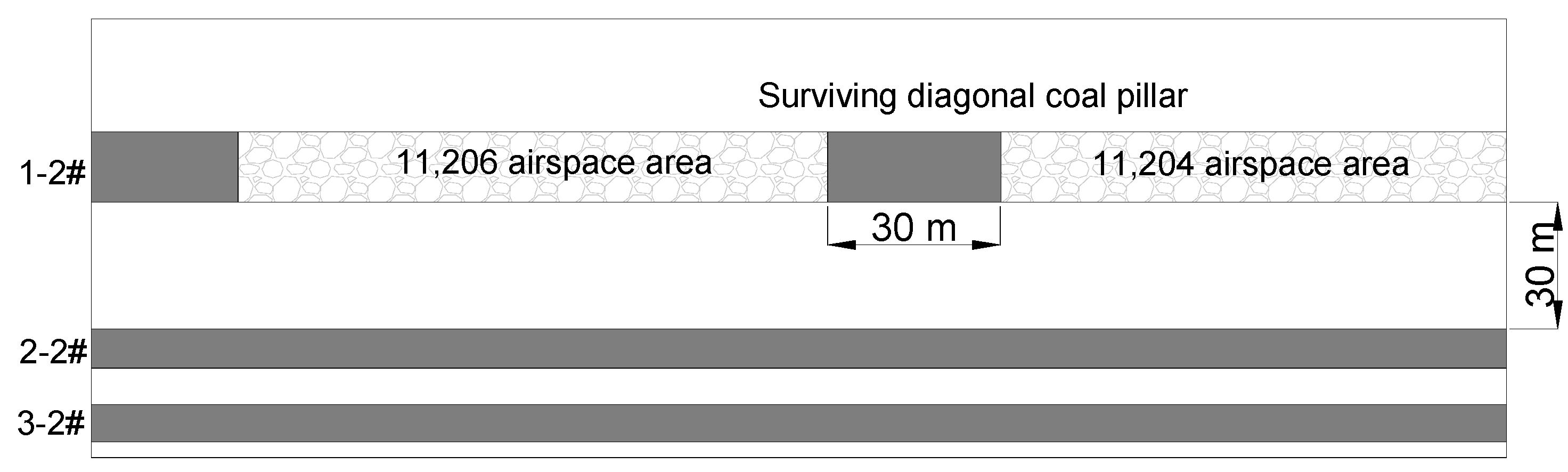
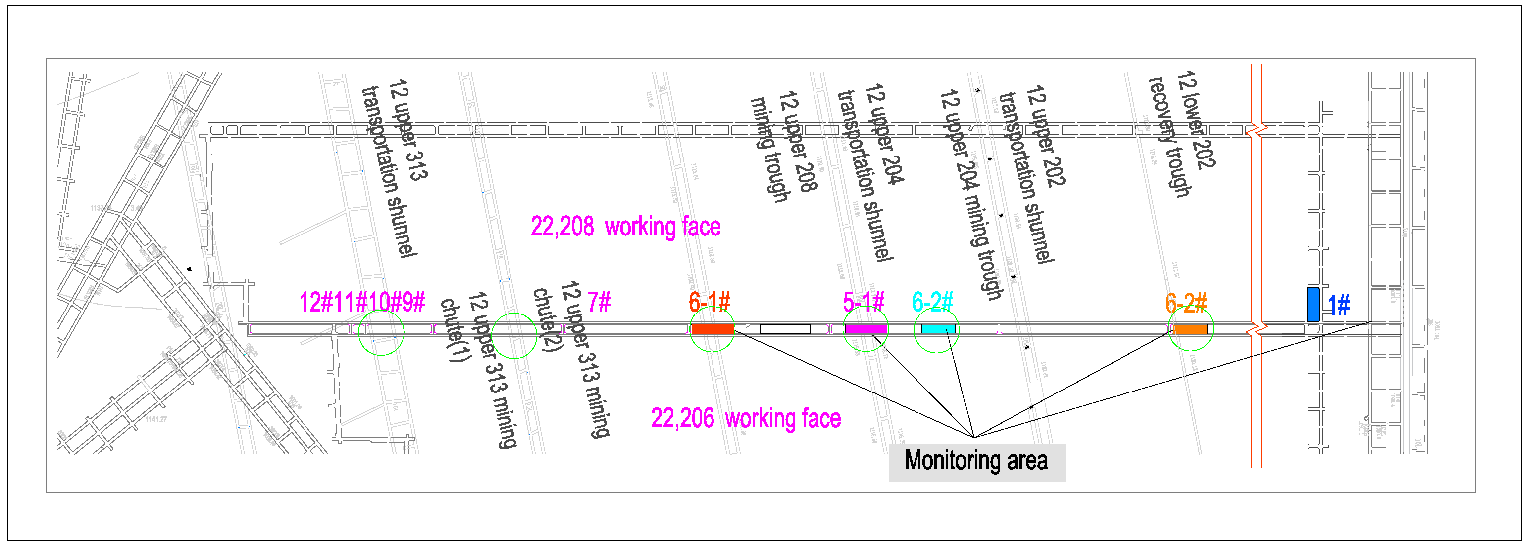
The Huojitu Mine in Daliuta is a typical example of close-distance coal seam mining, located on the Shaanxi side of the border between Shaanxi Province and the Inner Mongolia Autonomous Region, under the jurisdiction of Zhongji Township, Shenmu County. The eastern side of the 22,206 and 22,208 working faces is adjacent to the 2-2# coal seam’s south wing auxiliary transport main roadway in the second panel area, while the western side is adjacent to the 2-2# coal seam’s upper 301 return air measure roadway. The northern side borders solid coal seams, and the southern side is adjacent to the 22,204 working face. Influenced by the mining of the overlying 1-2# coal seam, numerous obliquely intersecting coal pillars, approximately 30 m wide, remain in the goaf. These oblique coal pillars overlap with the transportation roadway of the 22,206 working face and the return air roadway of the 22,208 working face in the underlying 2-2# coal seam, along with the section coal pillars laid out between them.

The layout of the working faces and the positions of the section coal pillars in the 2-2# coal seam are shown in Figure 1. The mine field contains seven mineable coal seams within the coal-bearing strata, with a total mineable thickness of 24.22 m, a minimum thickness of 5.87 m, and an average total thickness of 17.02 m. After the preliminary mining of the 1-2# coal seam, the remaining oblique coal pillars in the goaf affect the subsequent mineable 2-2# coal seam, which has an average interlayer spacing of 30 m from the overlying goaf. The schematic distribution of the coal seams is illustrated in Figure 2.

2.2. Fiber Bragg Grating Deployment

Fiber Bragg Gratings (FBGs) were inserted through boreholes into the section coal pillars located beneath the overlying goaf’s oblique coal pillars. Four monitoring stations were set up to observe the deformation of these section coal pillars, located between the 22,206 transportation roadway and the 22,208 return air roadway as shown in Figure 3. Upon completing the installation of the FBG sensors underground, communication fiber-optic cables were connected to the control room, forming a complete FBG strain monitoring loop for collecting the strain data of the section coal pillars.

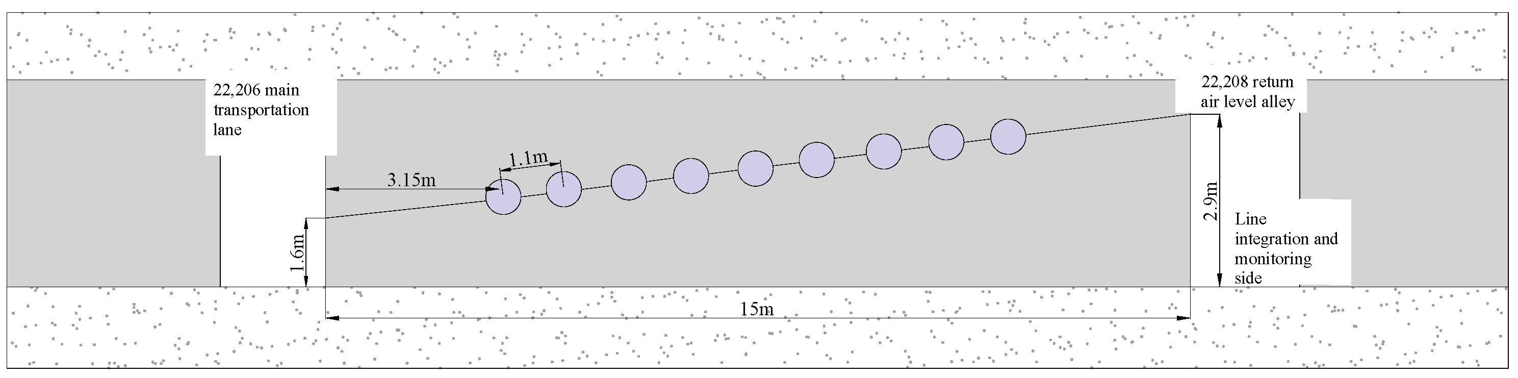
In practical engineering applications, to monitor the deformation of the section coal pillars in the 2-2# coal seam, FBG sensors were inserted into boreholes drilled at a 5° upward angle into the section coal pillars between the main transportation roadway of the 22,206 working face and the return air roadway of the 22,208 working face. Nine FBG strain monitoring points were arranged along the 15 m width of the section coal pillars, with the profile and layout of these nine points shown in Figure 4.

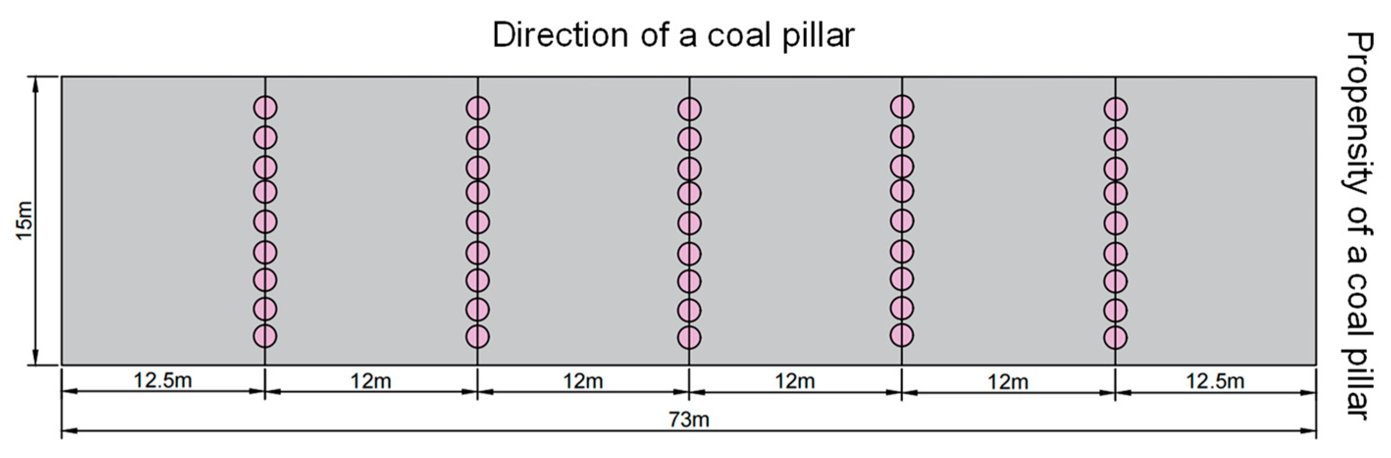
Five FBG arrays were installed along the strike direction of the section coal pillars. One array was placed in the center, with two arrays on each side in an axially symmetrical manner to monitor the shoulder areas of the bell-shaped load, aiming to capture deformation data from different positions along the inclination direction of the coal pillars. Based on the calculation of the influence range of the overlying oblique coal pillars from the 22,208 working face, which is 72.26 m, the 5-1# section coal pillar is located directly below these oblique pillars and within their influence range, exhibiting a bell-shaped load distribution. Enhanced monitoring was conducted at the central position of the 5-1# section coal pillar, with the process layout along its strike direction illustrated in Figure 5.

2.3. Monitoring Results and Analysis

According to the similarity laws, relevant site parameters were converted, resulting in an equivalent tunnel radius of α = 0.0342 m and an initial ground stress of P₀ = 156 kPa. Mechanical tests on the similar materials for coal yielded an elastic modulus E = 3.21 GPa, a Poisson’s ratio of 0.35, an expansion coefficient of the fracture zone of 1.4, an internal friction angle of 27.83°, and a residual cohesion of 0.624 MPa. These parameters were substituted into theoretical formulas for calculations, and the radial strain at the boundary between the elastic and plastic zones of the section coal pillar was determined to be 560 με, while the radial strain at the boundary between the fracture zone and the plastic zone was determined to be 1040 με. These values served as reference points for analyzing the distribution characteristics of the elastic–plastic regions of the coal pillar strain monitored by the Fiber Bragg Gratings (FBGs).

$$\left\{\begin{array}{c}{\mu }_e={\displaystyle \frac{1+\mu }{E}}\left[(1-2\mu )P_{0}r+(P_0-{\sigma }_r\left|r=R_s){\displaystyle \frac{R_s^2}{r}}\right.\right]\\ {\epsilon }_{re}={\displaystyle \frac{1+\mu }{E}}\left[\left(1-2\mu \right)P_0-(P_0-{\sigma }_r\left|r=R_s){\displaystyle \frac{R_s^2}{r^2}}\right.\right]\\ {\epsilon }_{\theta e}={\displaystyle \frac{1+\mu }{E}}\left[\left(1-2\mu \right)P_0+(P_0-{\sigma }_r\left|r=R_s){\displaystyle \frac{R_s^2}{r^2}}\right.\right]\end{array}\right.$$

(1)

$$\left\{\begin{array}{c}{\epsilon }_{rs}={\displaystyle \frac{1+\mu }{E}}(P_0-{\sigma }_r\left|r=R_s)\right.\left[{\displaystyle \frac{{\eta }_s-1}{{\eta }_s+1}}-{\displaystyle \frac{{2\eta }_s}{{\eta }_s+1}}({\displaystyle \frac{R_s}{r}}{)}^{1+{\eta }_s}\right]\\ {\epsilon }_{\theta s}={\displaystyle \frac{1+\mu }{E}}(P_0-{\sigma }_r\left|r=R_s)\right.\left[{\displaystyle \frac{{\eta }_s-1}{{\eta }_s+1}}-{\displaystyle \frac{2}{{\eta }_s+1}}({\displaystyle \frac{R_s}{r}}{)}^{1+{\eta }_s}\right]\end{array}\right.$$

(2)

$$\left\{\begin{array}{c}{\epsilon }_{rb}=-{\displaystyle \frac{1+\mu }{E}}(P_0-{\sigma }_r\left|r=R_s)\right.{\eta }_b\left[{\displaystyle \frac{{\eta }_s-1}{{\eta }_s+1}}-{\displaystyle \frac{2}{{\eta }_s+1}}({\displaystyle \frac{R_s}{R_b}}{)}^{1+{\eta }_s}\right]({\displaystyle \frac{R_b}{r}}{)}^{1+{\eta }_s}\\ {\epsilon }_{\theta b}={\displaystyle \frac{1+\mu }{E}}(P_0-{\sigma }_r\left|r=R_b)\right.\left[{\displaystyle \frac{{\eta }_s-1}{{\eta }_s+1}}-{\displaystyle \frac{2}{{\eta }_s+1}}({\displaystyle \frac{R_s}{R_b}}{)}^{1+{\eta }_s}\right]({\displaystyle \frac{R_b}{r}}{)}^{1+{\eta }_s}\end{array}\right.$$

(3)

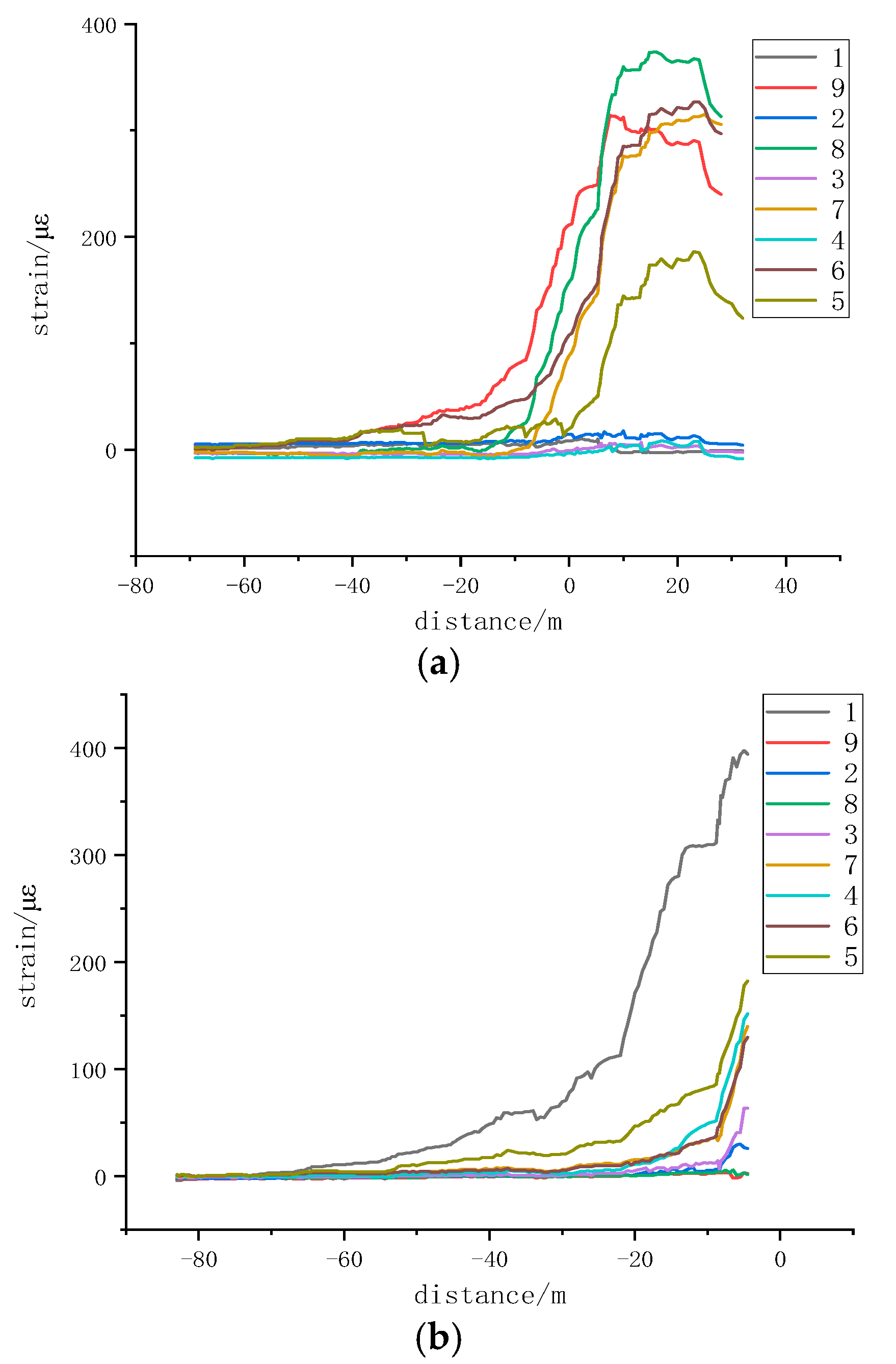
Figure 6 shows the deformation monitoring results of the 5-1# section coal pillar from 9 July to 29 July, based on monitoring points 1–9 from five FBG boreholes. The strain variation curve at monitoring points 1–9 in borehole 1 shows that with the advancement of the working face, the strain near the 22,208 working face rapidly increased due to the impact of mining stress on the underlying coal seam working face. The stress concentration effect gradually increased within about 10 m in front of the working face. Subsequently, the strain curve quickly decreased, indicating that the 5-1# section coal pillar was affected by the concentrated stress of the overlying oblique residual coal pillars. The deformation influence range was from the monitoring points 5 to 9 on the left side at 12.5 m, while there was almost no noticeable change in the range from monitoring points 1 to 4, differing from the strain variation patterns under vertical or parallel conditions of the overlying and underlying coal pillars.

The strain variation curve at monitoring points 1–9 in borehole 2 showed a steep increase in strain with the advancement of the working face. However, due to issues arising during actual construction, the monitoring point in borehole 2 broke about 5 m before the 22,208 working face reached the borehole opening, resulting in abnormal data collection. Given the bell-shaped load distribution of the 5-1# section coal pillar, the strain variation trend at borehole 4, which symmetrically aligns with borehole 2, was used for reference.

As the 22,208 working face advanced, the 5-1# section coal pillar was influenced by the advanced support pressure and lateral support pressure. The strain curves measured by the nine monitoring points in borehole 5 showed a sharp increase approximately 100 m from the coal wall. Using the theoretical values to analyze the elastic–plastic zoning range within the coal pillar width, the monitoring points 8 and 9 reached the plastic zone approximately 178 m from the borehole opening. It was determined that the entire area of borehole 3 along the width of the section coal pillar was affected by the concentrated stress of the overlying oblique residual coal pillars, covering the left side at 36.5 m.

From the strain monitoring data of borehole 4, it was observed that during the retreat of the 22,208 working face, the strain monitoring values showed small variations. The strain curve first increased steeply, then dropped sharply, and later increased before leveling off. The position of borehole 4, located in the central right region of the 5-1# section coal pillar, showed a stress trend of first increasing and then decreasing, consistent with the actual measured strain variation trend.

The strain monitoring data of borehole 5 indicated a gradual increase in strain with the mining activities of the 22,208 working face. At this stage, the 22,208 working face was farther from the overlying oblique residual coal pillars, resulting in minimal deformation, suggesting it was at the edge of the influence zone of the overlying oblique residual coal pillars. This area of the section coal pillar showed minor deformation, remaining relatively stable. It was also inferred that the 5-1# section coal pillar was influenced by the concentrated stress of the overlying oblique residual coal pillars, with the deformation influence range at 12.5 m on the right side between monitoring points 4 and 7. However, unlike the symmetrically arranged borehole 1, the monitoring range included point 4 but excluded points 8 and 9, indicating that the influence zone of the overlying oblique residual coal pillars shifted towards the goaf on the 22,206 side.

3. Data Denoising

3.1. Data Decomposition

One drawback of the empirical mode decomposition (EMD) method is the presence of mode mixing, which means that multiple frequency components can exist within a single intrinsic mode function (IMF). Ensemble empirical mode decomposition (EEMD) is a novel decomposition algorithm that improves upon EMD based on empirical validation. EEMD involves adding Gaussian white noise to the original signal sequence and then averaging the intrinsic mode function components. The intermittent phenomena of the original signal can be eliminated by the statistical characteristics of the white noise’s uniform frequency distribution, thereby suppressing the mode mixing effect of EMD and improving the decomposition efficiency and accuracy. The principle is as follows:

Step 1: Add a random Gaussian white noise sequence to the original signal, i.e.,

$$x_n\left(t\right)=x\left(t\right)+k{m}_n(t)$$

(4)

In the equation, k is the amplitude coefficient of the added Gaussian white noise sequence.

Step 2: Decompose the signal with the added Gaussian white noise using EMD to obtain a set of the IMF.

Step 3: Repeat the above two steps n times and compute the average of the IMF components obtained from each decomposition to eliminate the influence of Gaussian white noise on the true IMF components. The final obtained IMF components and the residual r(t) are, respectively, as follows:

$$c_j\left(t\right)={\displaystyle \frac{1}{n}}\sum _{i=1}^n{c}_{ij}\left(t\right)$$

(5)

$$r\left(t\right)={\displaystyle \frac{1}{n}}\sum _{i=1}^n{r}_i\left(t\right)$$

(6)

In the equation, c_j(t) is the j-th IMF component obtained from the ensemble empirical mode decomposition of the original signal.

Step 4: Finally, the original signal is represented as follows:

$$x\left(t\right)=\sum _{j=1}^k{c}_j\left(t\right)+r(t)$$

(7)

3.2. Threshold Determination (DE) Algorithm

In signal reconstruction, handling inappropriate IMF components can cause signal distortion and reduce data accuracy. Therefore, dispersion entropy is introduced to assess the proportion of noise in high-frequency and low-frequency components of sample data. The DE algorithm is fast and considers the relationship between amplitudes, effectively addressing issues such as abrupt changes in similarity measures and discrepancies between amplitude means and values. The calculation process is as follows:

• Map the time series x, x= {x_i = 1, 2, …, N} to y, y = {y_j}, using a normal distribution function as shown in Equation (8), where uuu represents the mean and σ represents the variance.

$$y_i={\displaystyle \frac{1}{\sigma \sqrt{2\pi }}}{\int }_{-\infty }^{x_i}{e}^{{\displaystyle \frac{-(t-\mu {)}^2}{2{\sigma }^2}}}dt$$

(8)

2.

Use linear transformation to map y to the range {1, 2, …, x} as shown in Equation (9), where R is the rounding function and c is the number of categories.

$$Z_j^c=R(c·y_j+0.5)$$

(9)

3.

Calculate the embedding vector $Z_i^{\left(m,c\right)}$ as shown in Equation (10). m is the embedding dimension, and d is the time delay, where $i=1, 2, ...,N-(m-1)d$.

$$Z_i^{(m,c)}=\{Z_i^c,Z_{i+d}^c,\dots ,Z_{i+\left(m-1\right)d}^c\}$$

(10)

4.

Calculate the probability of each dispersion pattern, as shown in Equation (11), where Number(π_{v0, v1,…,vm-1}) represents the number of embedding vectors mapped to the dispersion pattern.

$$p\left({\pi }_{v_0{, v}_1,\dots , v_m}\right)={\displaystyle \frac{Number({\pi }_{v_0,v_1,\dots , v_m})}{N-(m-1)d}}$$

(11)

5.

According to the definition of Shannon entropy, the dispersion entropy value of the original signal x is defined as shown in Equation (12):

$$DE\left(x,m,c,d\right)=-\sum _{\pi =1}^{c^m}p({\pi }_{v_{0,}{v}_1,\dots , v_{m-1}})·\mathrm{l}\mathrm{n}(p({\pi }_{v_{0,}{v}_1,\dots , v_{m-1}}))$$

(12)

The larger the dispersion entropy value, the higher the complexity of the time series; conversely, a smaller value indicates lower complexity. If the dispersion entropy value of the IMF components of the strain data is large, it proves that the complexity of the IMF components is higher and contains more noise signals. Conversely, it proves that the IMF component contains useful information from the original time series. Therefore, when the dispersion entropy values of adjacent IMFs change abruptly, it indicates a sharp increase or decrease in the noise content between the two IMF components. In this paper, the threshold point is denoted as M. The dispersion entropy values and the ratio of the dispersion entropy values of adjacent IMFs are calculated for each IMF component obtained from the EEMD decomposition.

3.3. Singular Value Decomposition (SVD)

Singular value decomposition (SVD) is a numerical processing method. According to mathematical linear theory, for any real matrix $A\in R^{m\times n}$ of arbitrary dimensions with rank r = min(m, n), there exist orthogonal matrices $U\in R^{m\times n}$ and $V\in R^{m\times n}$ such that the following equation holds:

$$A=US{V}^T$$

(13)

In the equation, A is the matrix to be decomposed, $U=\left(u_1,u_2,...,u_m\right)\in R^{m\times n},\mathrm{and}{u}_i$ are the column vectors of U, forming the left singular matrix; $V=\left(v_1,v_2,...,v_m\right)\in R^{m\times n},\mathrm{a}\mathrm{n}\mathrm{d} v_i$ are the column vectors of V, known as the right singular matrix; S is the diagonal matrix composed of singular values. $S=\left[\begin{array}{cc}{S}_1& 0\\ 0& 0\end{array}\right],S_1=diag({\sigma }_1,{\sigma }_2,...,{\sigma }_r)$, and ${\sigma }_1\ge {\sigma }_2\ge ...\ge {\sigma }_r>0$. Singular values have good stability, scale invariance, and rotation invariance, and they are intrinsic features of the matrix.

4. Denoising and Prediction of Optical Fiber Monitoring Signals Based on EEMD-DE-SVD and DBO-LSTM-BP

4.1. Denoising Model

This paper uses the actual deformation optical fiber grating monitoring data from the 5-1# coal pillar between the 22,206 and 22,208 working faces of the Huojitu Well 2-2# coal seam in the Daliuta Coal Mine during secondary mining as experimental data. The optical fiber grating at borehole 3 is located in the center of the 5-1# coal pillar, i.e., the middle of the bell-shaped load distribution area, where the impact of the residual inclined coal pillar from the overlying mined-out area is more extensive and the concentrated stress effect is stronger. From the deformation monitoring strain curve of the above section coal pillar, it is evident that the initial optical fiber grating monitoring data are disturbed by noise, resulting in spikes and redundant signals, requiring the denoising of the original optical fiber grating signal. However, the optical fiber grating at boreholes 1–5 is located at different positions under the residual inclined coal pillar from the overlying mined-out area, leading to varying levels of noise interference in the deformation monitoring of the coal pillar section. Additionally, the noise interference in curves with larger strain variations can increase the complexity of the noise signal.

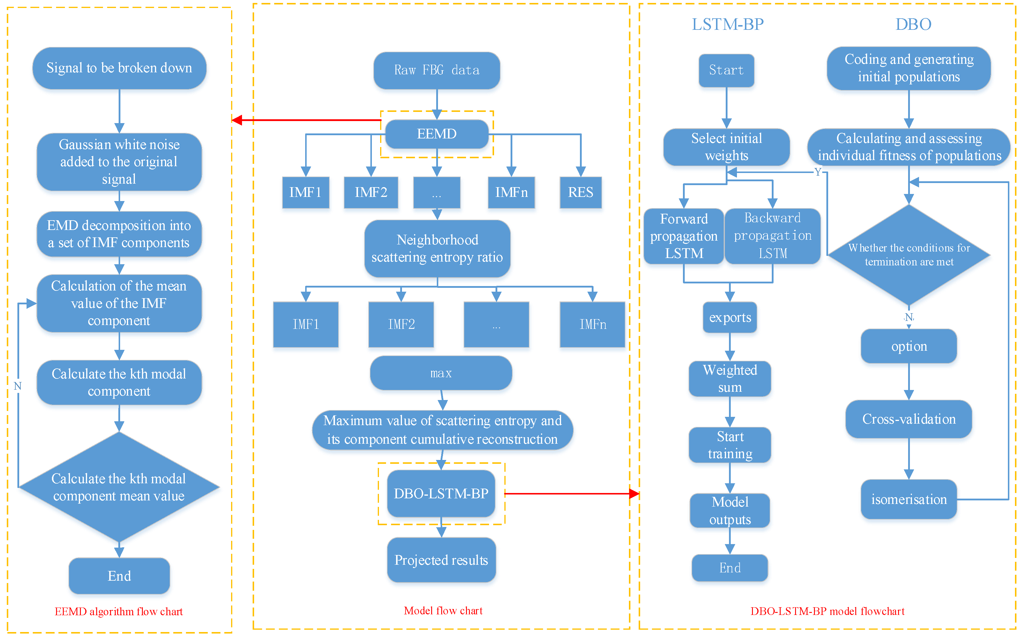
Denoising steps for optical fiber signals based on EEMD-DE-SVD are as follows:

Step 1: Collect vibration signals under various working conditions.

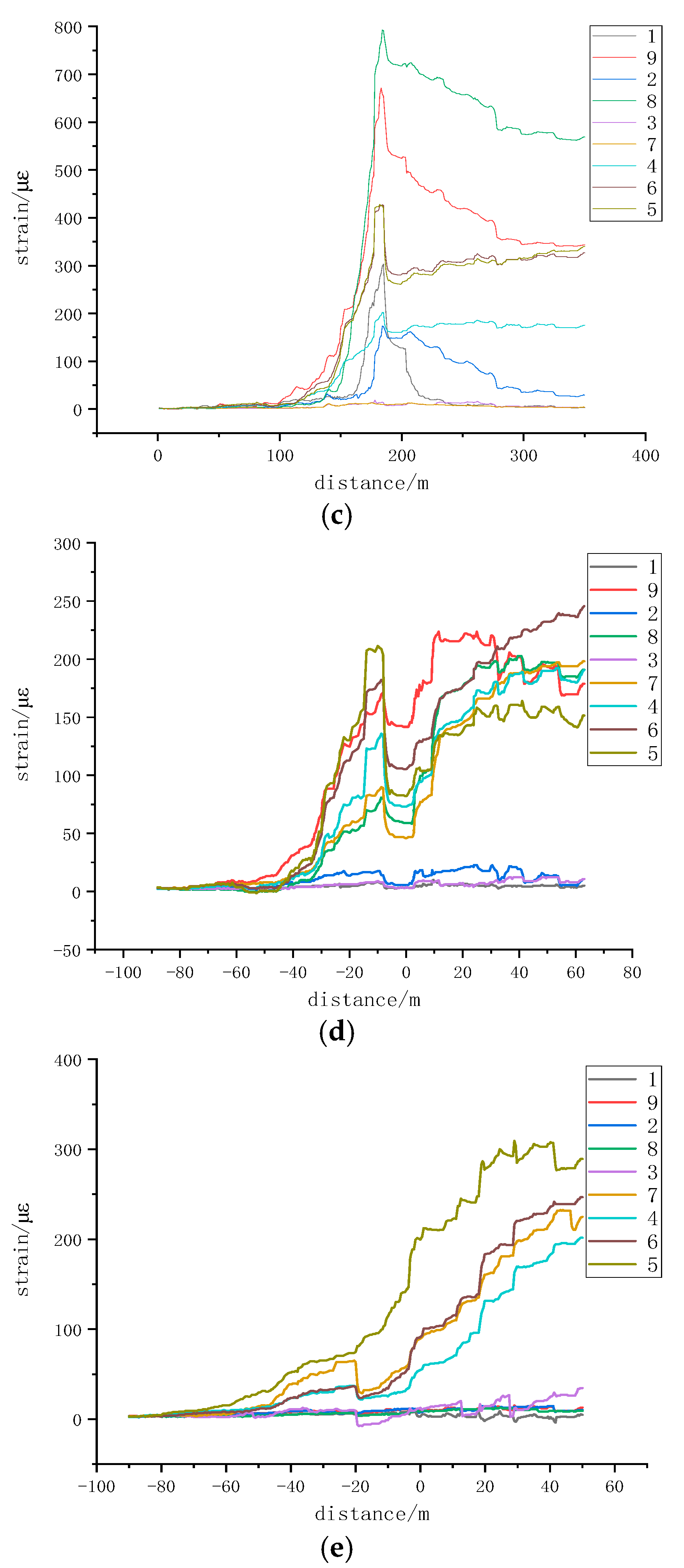
Step 2: Use EEMD to decompose vibration signals under different working conditions. For example, perform ensemble empirical mode decomposition on the signal from borehole 1, measurement point 8, and obtain the first 6 IMF components as shown in Figure 7.

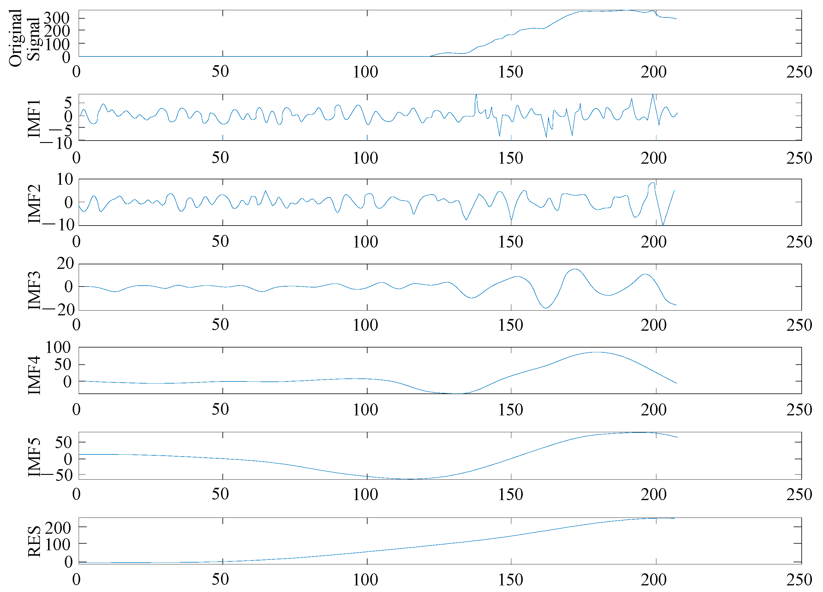
Step 3: Calculate the dispersion entropy values of each IMF component using the DE algorithm, as shown in Figure 8.

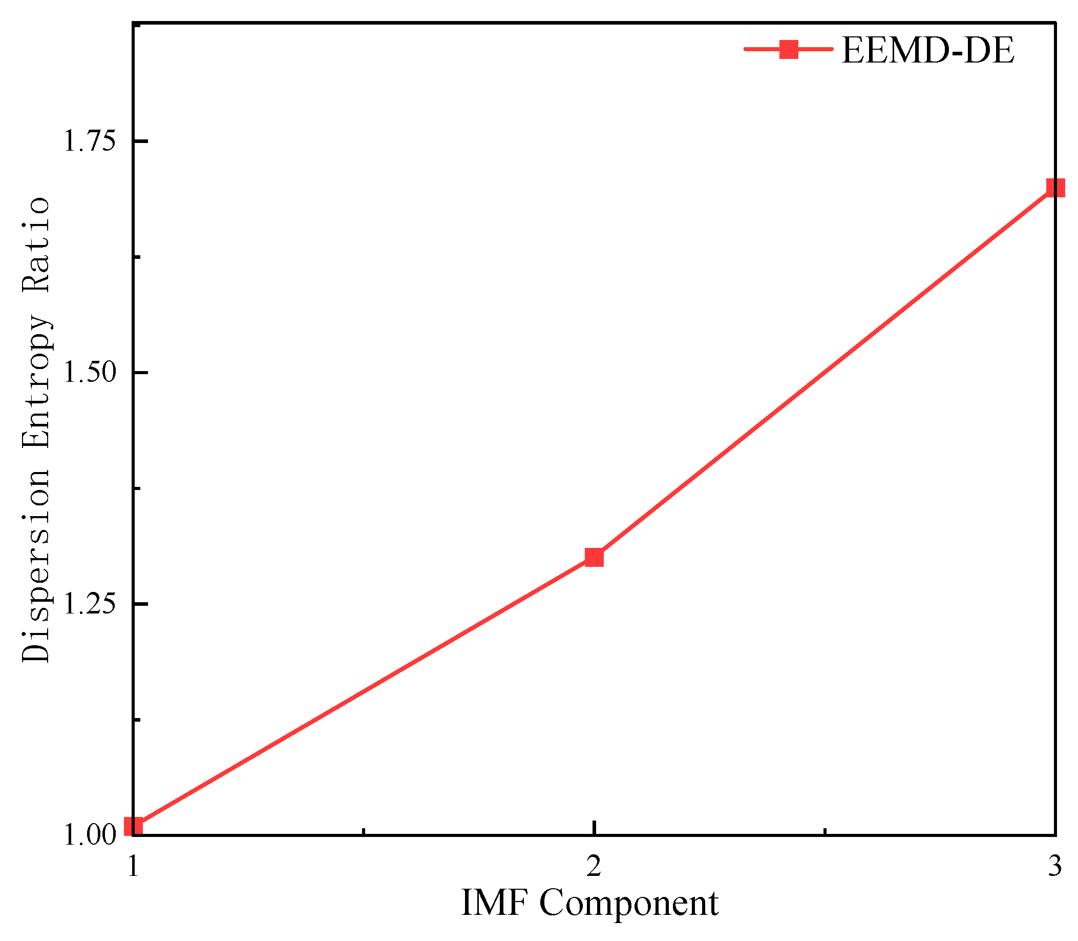
Step 4: Calculate the ratio of adjacent IMF dispersion entropy values, as shown in Figure 9.

Step 5: The threshold critical point M1 for the EEMD denoising algorithm is 1.700. M1 is the dispersion entropy ratio between IMF3 and IMF4. The maximum ratio indicates a sharp decrease in noise content, suggesting that IMF4 and subsequent components contain less noise. Therefore, IMF1–IMF3, which contain higher noise levels, should be discarded. Use IMF4–IMF5 and the residual component RES for data reconstruction.

Step 6: Perform singular value decomposition (SVD) on the matrix constructed from the denoised signal using the DE algorithm, and use the results as feature vectors.

4.2. Prediction Model

This paper combines LSTM and BP neural network algorithms. The computer is configured with Windows 10, using PyCharm 2021.2.2 and the TensorFlow 2.2 deep learning framework, with training and testing sets divided in an 8:2 ratio. The model employs a three-layer LSTM network structure and a two-layer BP neural network structure. Due to the difficulty of manual parameter optimization under these conditions, the dung beetle optimization (DBO) algorithm is introduced to optimize the parameters of the combined neural network structure.

The goal of the DBO algorithm is to find the x that minimizes (or maximizes) the objective function f(x). This algorithm is known for its strong search capabilities and adaptability, making it widely used in machine learning, deep learning, and other fields.

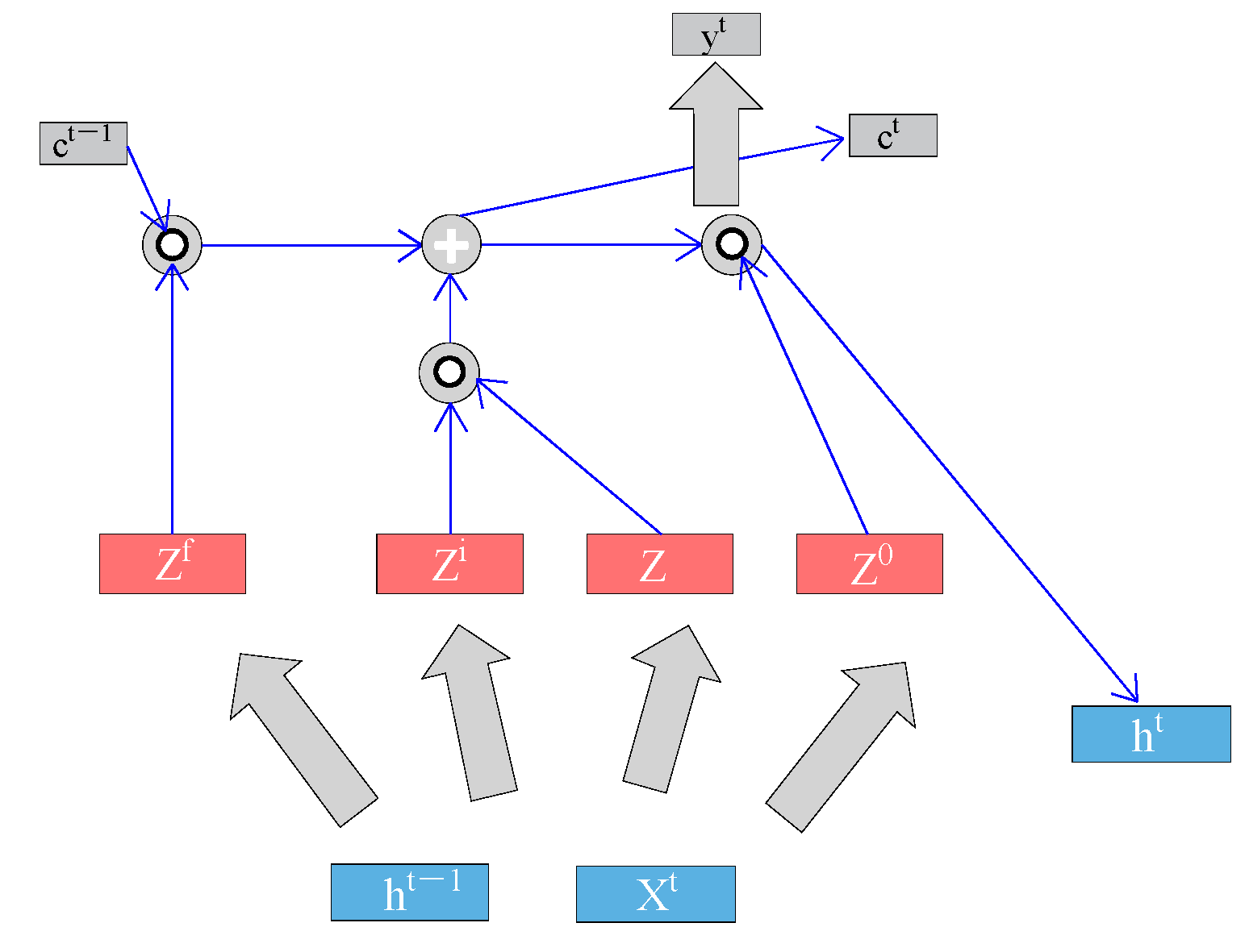
LSTM (long short-term memory) is a special type of recurrent neural network (RNN) with a structure designed to learn long-term dependencies, as shown in Figure 10. The LSTM introduces three special “gates” that provide its long-term memory capability. The input gate updates the cell state based on the current input and the previous hidden state, while the forget gate selectively forgets information to prevent minor details from affecting the predictions. The output gate outputs a hidden state that includes information from the previous input, which, along with the current input, is passed to the input gate of the next unit, facilitating the information transfer and enabling the model to maintain memory.

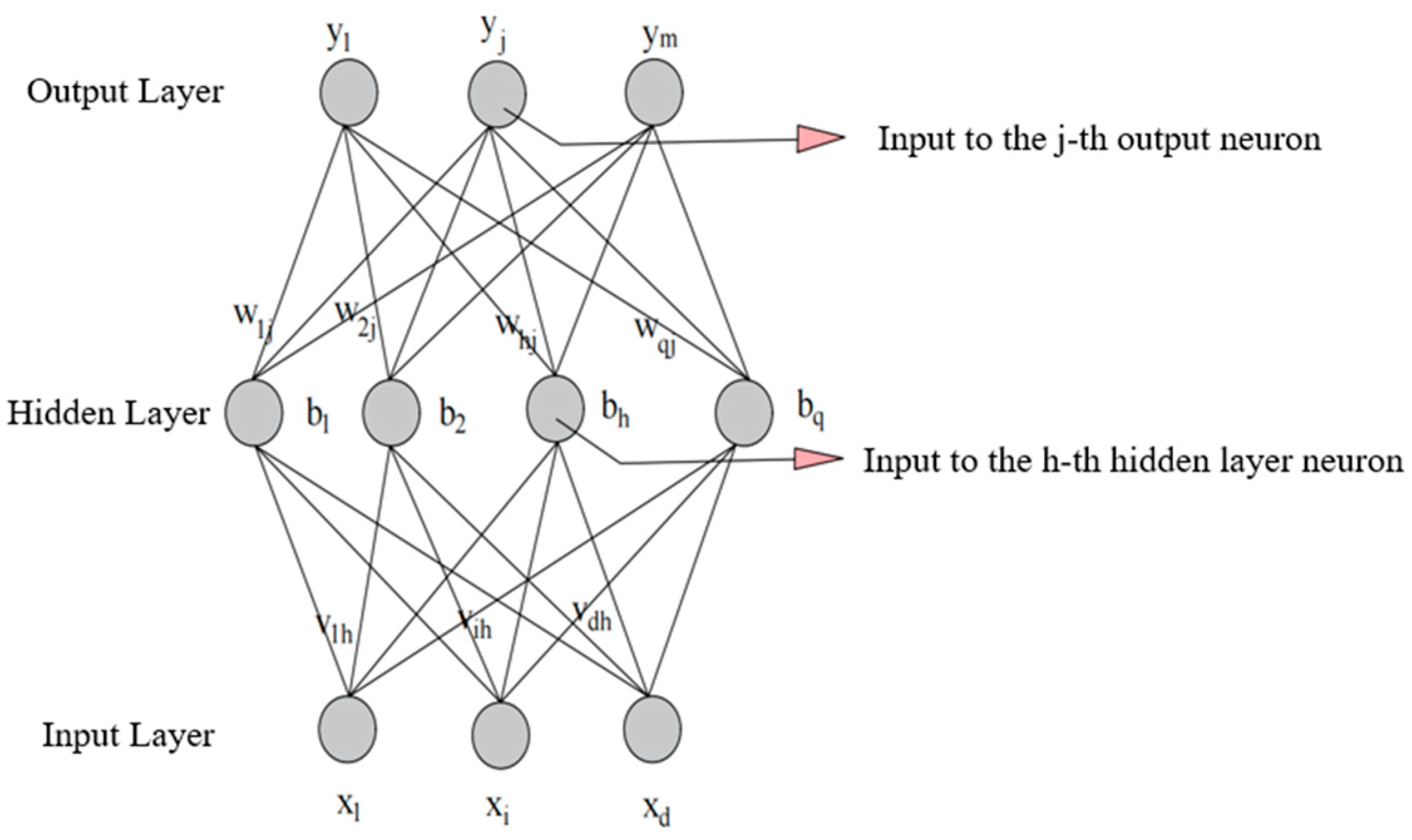
The BP neural network consists of an input layer, a hidden layer, and an output layer. The input layer is the entry point for information, the hidden layer is where information is processed, and the output layer provides the final result. The process of the BP neural network is mainly divided into two stages: the first stage is the forward propagation of the signal, from the input layer through the hidden layer to the output layer; the second stage is the backward propagation of the error, from the output layer to the hidden layer and finally to the input layer, sequentially adjusting the weights and biases from the hidden layer to the output layer and from the input layer to the hidden layer. Figure 11 is a schematic diagram of the neural network layers.

The BP neural network model has high requirements for the quality of data preprocessing and requires a large number of iterative calculations during the training process, which can easily lead to local optima and difficulty in converging to the global optimum. Section 2.1 describes that the EEMD-DE-SVD algorithm can decompose and denoise the signal, improving the quality of data preprocessing. The DBO algorithm can find the global optimum in the search space. However, when applying genetic algorithms to specific problems, there is no standard hyperparameter setting rule, so hyperparameter optimization is needed during model training iterations to find suitable hyperparameters. Additionally, the BP neural network model faces the problem of gradient disappearance due to gradient propagation, which causes slow convergence between the actual values and error values. Therefore, this paper introduces the LSTM (long short-term memory) network to avoid the gradient disappearance problem.

Figure 12 shows the combined neural network prediction model incorporating the above four algorithms. To verify the prediction performance of this model, the actual deformation optical fiber monitoring data from the 5-1# coal pillar section of the Daliuta Huojitu Well is used for model training and testing.

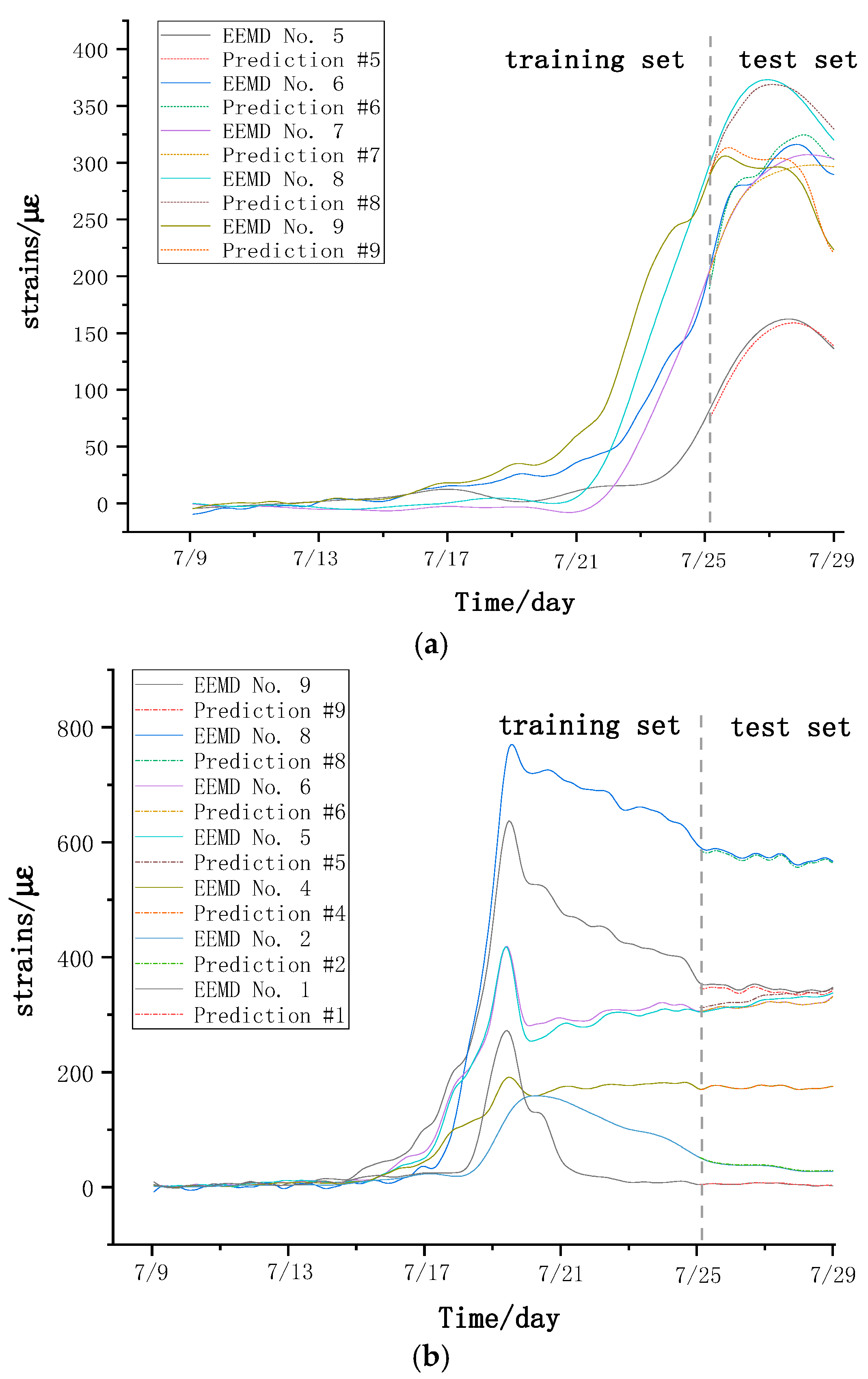
4.3. Prediction Results

The computer is configured with Windows 10, 32 GB of RAM, using the PyCharm 2021.2.2 and TensorFlow 2.2 deep learning framework. The training and testing sets are divided in an 8:2 ratio. The deformation of the 5-1# coal pillar section affected by secondary mining and the residual inclined coal pillar from 25 July to 29 July has been predicted. This section divides the mining of the 22,208 working face into three stages: the advance, passing, and retreat of the overlying residual inclined coal pillar. The prediction model established in Section 4.1 is used to forecast the deformation strain trend of the 5-1# coal pillar section for the current mining stage. The prediction results are shown in Figure 13.

4.4. Accuracy Evaluation Metrics

According to the model prediction results, the denoising prediction model’s output strain curve is closely aligned with the original curve and shows minimal deviation from the actual values. To evaluate the accuracy of the prediction model, four common error metrics are used: Absolute Error (MAE), Mean Squared Error (MSE), Root Mean Squared Error (RMSE), and the Linear Regression Correlation Coefficient (R²). The calculation formulas are shown in Equations (14)–(17). Among them, smaller values for MAE, MSE, and RMSE are better, while R² values range from 0 to 1, with values closer to 1 indicating better curve fitting. The metric values reflect how well the prediction curve fits the actual curve and indicate the prediction accuracy, where $y_i$ represents the original data and ${\hat{y}}_i$ represents the fitted data.

$$MAE={\displaystyle \frac{1}{n}}\sum _{i=1}^n\left|y_i-\widehat{y_i}\right|$$

(14)

$$MSE={\displaystyle \frac{1}{n}}\sum _{i=1}^m{(y}_i-\widehat{y_i}{)}^2$$

(15)

$$RMSE=\sqrt{{\displaystyle \frac{1}{n}}\sum _{i=1}^n{(y}_i-\widehat{y_i}{)}^2}$$

(16)

$$R^2=1-{\displaystyle \frac{\sum _{i=1}^n{(y}_i-\widehat{y_i}{)}^2}{\sum _{i=1}^n{(y}_i-\overline{y_i}{)}^2}}$$

(17)

4.5. Result Analysis

The evaluation metric results for strain monitoring boreholes 1, 3, 4, and 5 are shown in

Table 1. Evaluation index of strain prediction result of No.1 hole of coal pillar in 5-1# section.

Monitoring Point	MAE	MSE	RMSE	R2
5	6.25	50.99	7.14	0.88
6	7.76	82.16	9.06	0.89
7	4.96	37.12	6.09	0.88
8	6.03	44.01	6.63	0.89
9	6.93	55.31	7.44	0.89

,

Table 2. Evaluation index of strain prediction result of No.3 hole of coal pillar in 5-1# section.

Monitoring Point	MAE	MSE	RMSE	R2
1	0.29	0.13	0.36	0.94
2	1.19	1.75	1.32	0.95
4	0.53	0.40	2.63	0.93
5	1.20	1.96	1.40	0.95
6	1.16	1.86	1.36	0.92
8	1.01	1.63	1.22	0.95
9	1.13	0.98	1.52	0.94

,

Table 3. Evaluation index of strain prediction result of No.4 hole of coal pillar in 5-1# section.

Monitoring Point	MAE	MSE	RMSE	R2
4	1.15	0.15	1.51	0.94
5	1.02	1.12	1.06	0.95
6	1.86	1.91	0.22	0.95
7	0.29	0.10	0.31	0.98
8	1.05	1.51	1.23	0.96
9	1.34	2.80	1.67	0.97

and

Table 4. Evaluation index of strain prediction result of No.5 hole of coal pillar in 5-1# section.

Monitoring Point	MAE	MSE	RMSE	R2
4	0.56	0.98	0.42	0.99
5	1.52	0.33	0.54	0.98
6	0.24	0.62	0.35	0.99
7	0.81	1.42	0.63	0.98

.

Figure 13 shows the comparison between predicted and actual monitoring values at different advancement distances of the working face. When the working face advanced to approximately 1360.5 m, a small peak in strain at monitoring point 9, close to the 22,208 working face mining side, was observed. At this point, the MAE, MSE, RMSE, and R² were 6.93, 55.31, 7.44, and 0.89, respectively. The MAE, MSE, and RMSE values were relatively small, and the R² value of 0.89 was close to 1, indicating an accuracy of approximately 88%.

When the working face advanced to 1382.5 m, entering the stage of passing the residual inclined coal pillar, the strain trend prediction curves for the seven monitoring points had R² values around 0.95, with an accuracy of about 95%.

When the working face advanced to 1436.5 m, entering the stage of retreating from the residual inclined coal pillar, the strain curves showed an increasing trend. However, the deformation of the coal pillar in this area was relatively small and remained in a stable range. The actual strain curve and the predicted curve had minimal deviation, with the R² values for the strain trend prediction curves around 0.96, indicating an accuracy of about 96%.

When the working face advanced to 1440 m, despite being in the retreat stage, it was still on the edge of the residual inclined coal pillar influence zone. At this stage, the R² values for the strain trend prediction curves were around 0.99, with an accuracy of approximately 99%.

The predicted strain trend results for the coal pillar section ranged between 88% and 99%, confirming the feasibility and accuracy of the EEMD-DE-SVD-DBO-LSTM-BP denoising prediction model for forecasting the optical fiber strain monitoring data of the underlying coal pillar section when passing through the residual inclined coal pillar. This model can achieve a certain degree of the advanced prediction of coal pillar deformation strain.

5. Conclusions

In this paper, the internal deformation of section coal pillar is monitored by fiber grating sensing technology, and a prediction model of section coal pillar deformation is constructed by combining machine learning. The model is applicable to the conditions of shallow buried close coal seam section coal pillar stability monitoring, working face mining on section coal pillar internal deformation monitoring and broken ring prediction. In addition, the model combines two noise reduction algorithms, which helps to improve the prediction accuracy of the model. The accuracy and reliability of the DBO-LSTM-BP prediction model is confirmed by comparing it with the measured data in the field. The main findings of this study are summarized as follows:

(1)

Background and Monitoring: Using the 22,206 and 22,208 working faces of the Daliuta Huojitu Well as the background, embedded optical fiber grating sensors were introduced to achieve the real-time monitoring of internal deformation strain changes in the coal pillar section.

(2)

Stress Influence and Deformation Trends: As the working face advanced beneath the overlying residual inclined coal pillar, the area of concentrated stress influence further shifted towards the inclined coal pillar side. The overall impact area exhibited an approximately “diamond-shaped” influence, with the width of the peak strain region initially increasing and then decreasing.

(3)

Effectiveness of Denoising Algorithm: Using the EEMD-DE-SVD denoising algorithm, the Signal-to-Noise Ratio (SNR) increased by an average of 0.8 dB to 2.3 dB, and the Root Mean Square Error (RMSE) decreased by an average of 1.02 to 2.33, validating the effectiveness of the EEMD-DE-SVD denoising algorithm.

(4)

Prediction Model Accuracy: The EEMD-DE-SVD-DBO-LSTM-BP model was used to predict optical fiber grating strain signals. According to the results, the prediction accuracy of the EEMD-DE-SVD-DBO-LSTM-BP model ranged from 88% to 99%, demonstrating the effectiveness of this denoising prediction model.