
RSTSRN: Recursive Swin Transformer Super-Resolution Network for Mars Images


Abstract
1. Introduction
2. Related Works
2.1. Multiple-Image SR Algorithms
2.2. Single-Image SR Algorithms
2.2.1. Shallow Learning-Based SR Algorithms
2.2.2. Deep Learning-Based SR Algorithms
3. Materials and Methods
3.1. RSTSRN Architecture
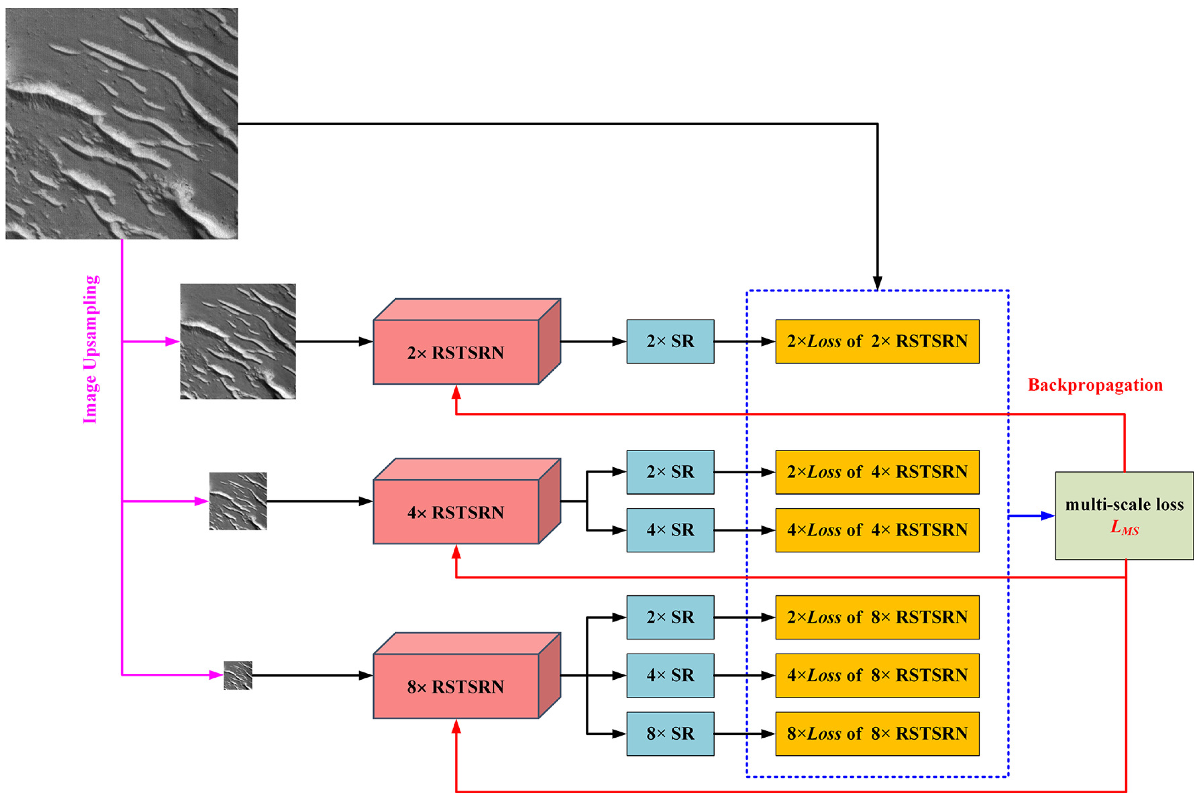
3.2. Loss Functions and Multi-Scale Training Strategy
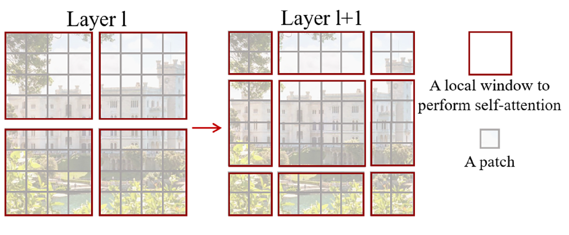
3.3. Shifted Window
3.4. Training and Testing
4. Results
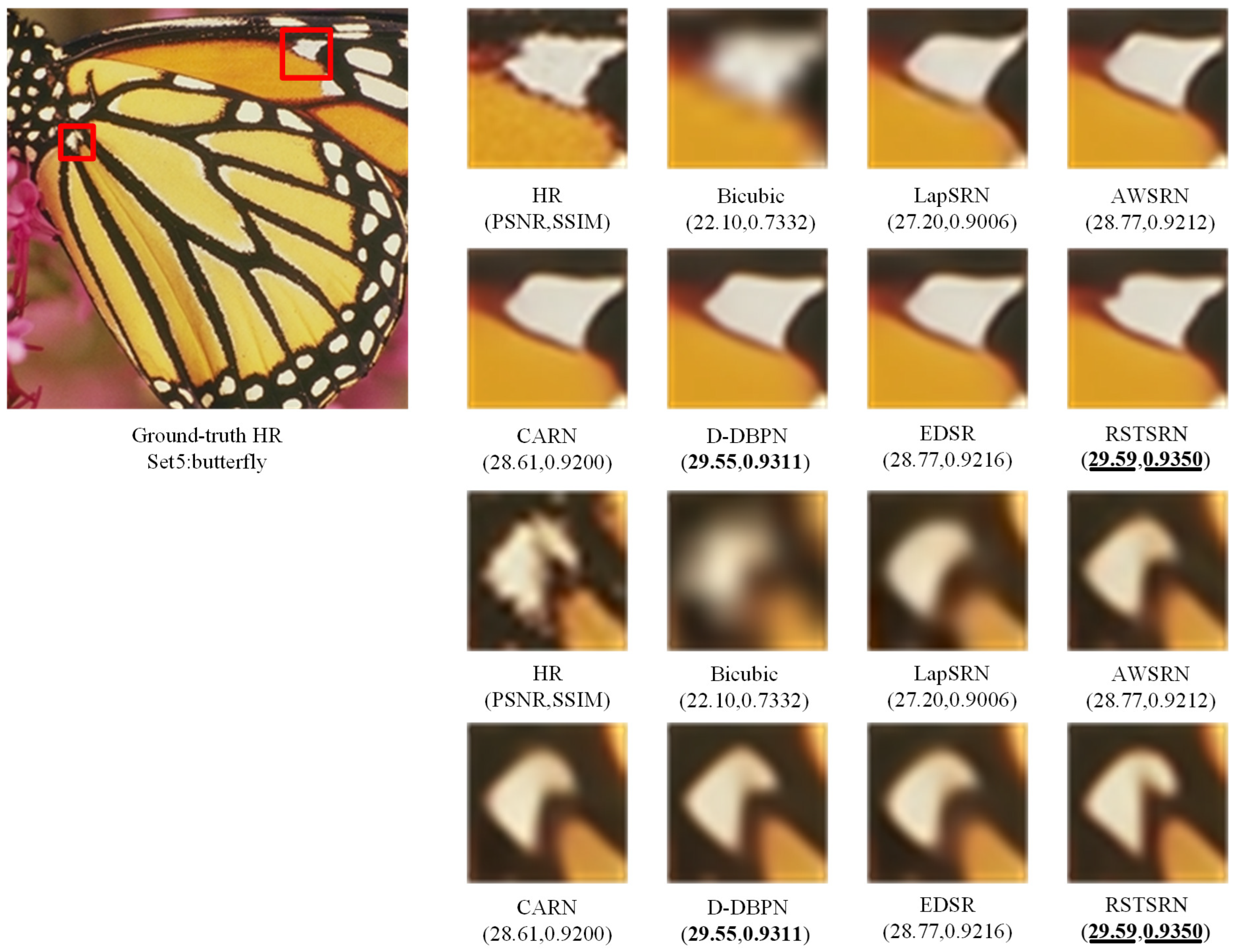
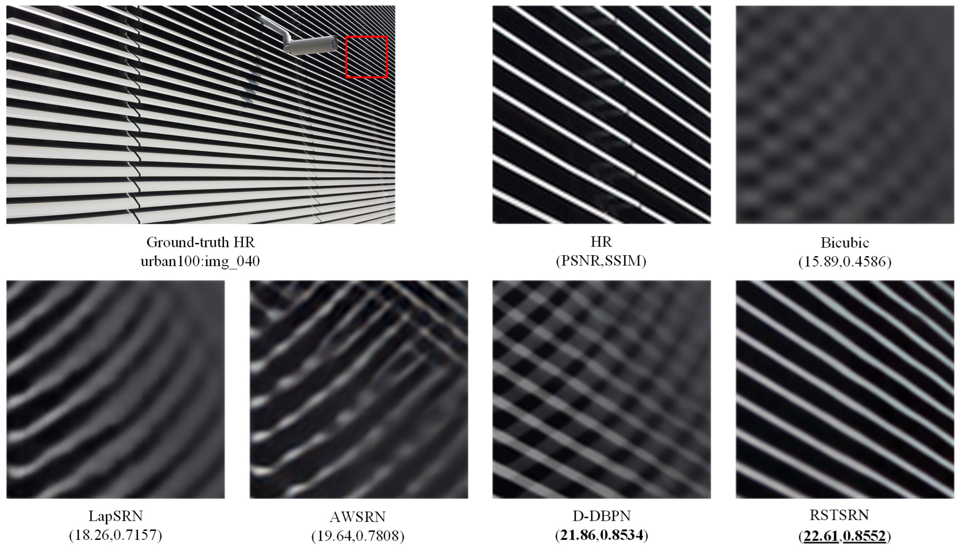
4.1. RSTSRN Results for Natural Images
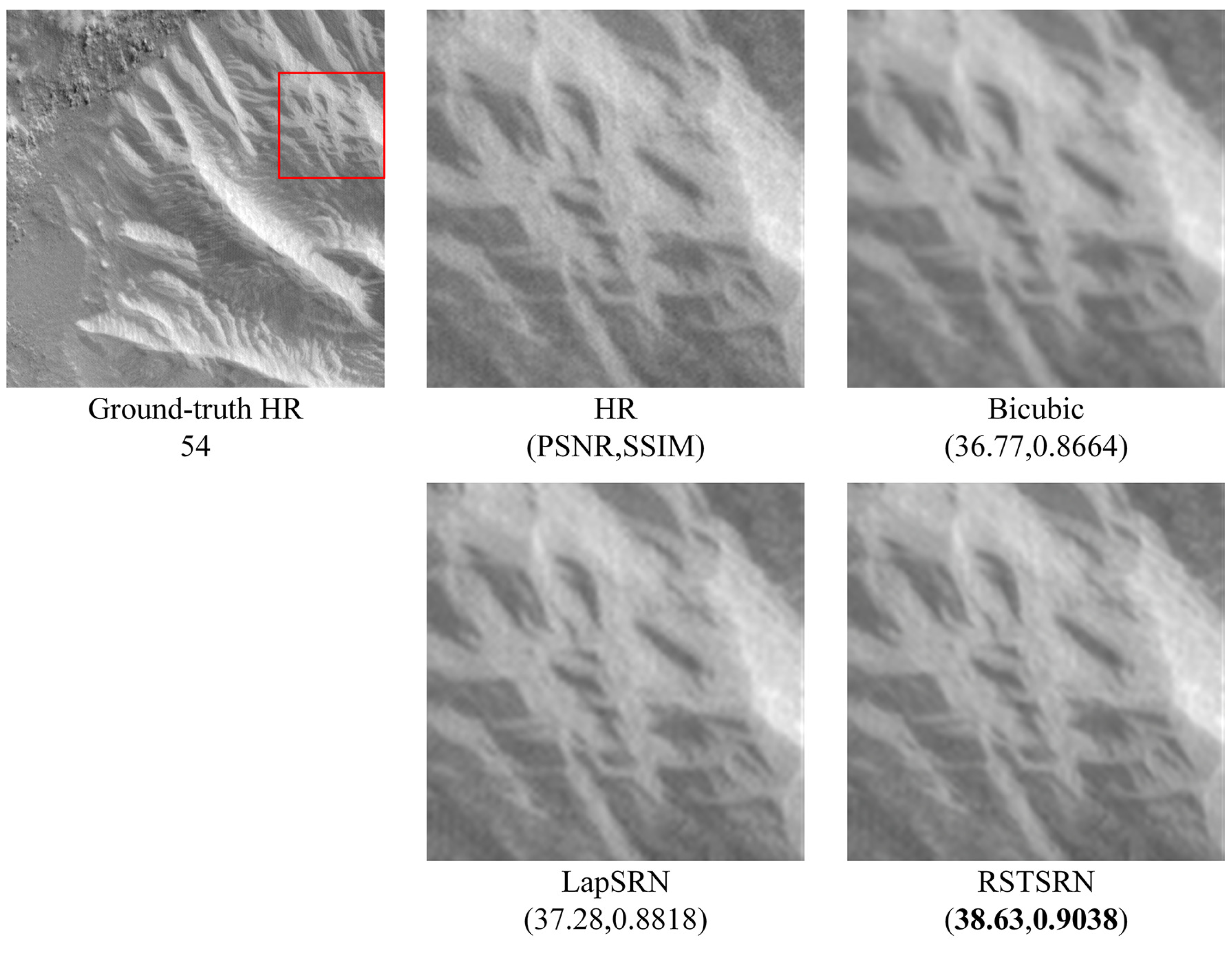
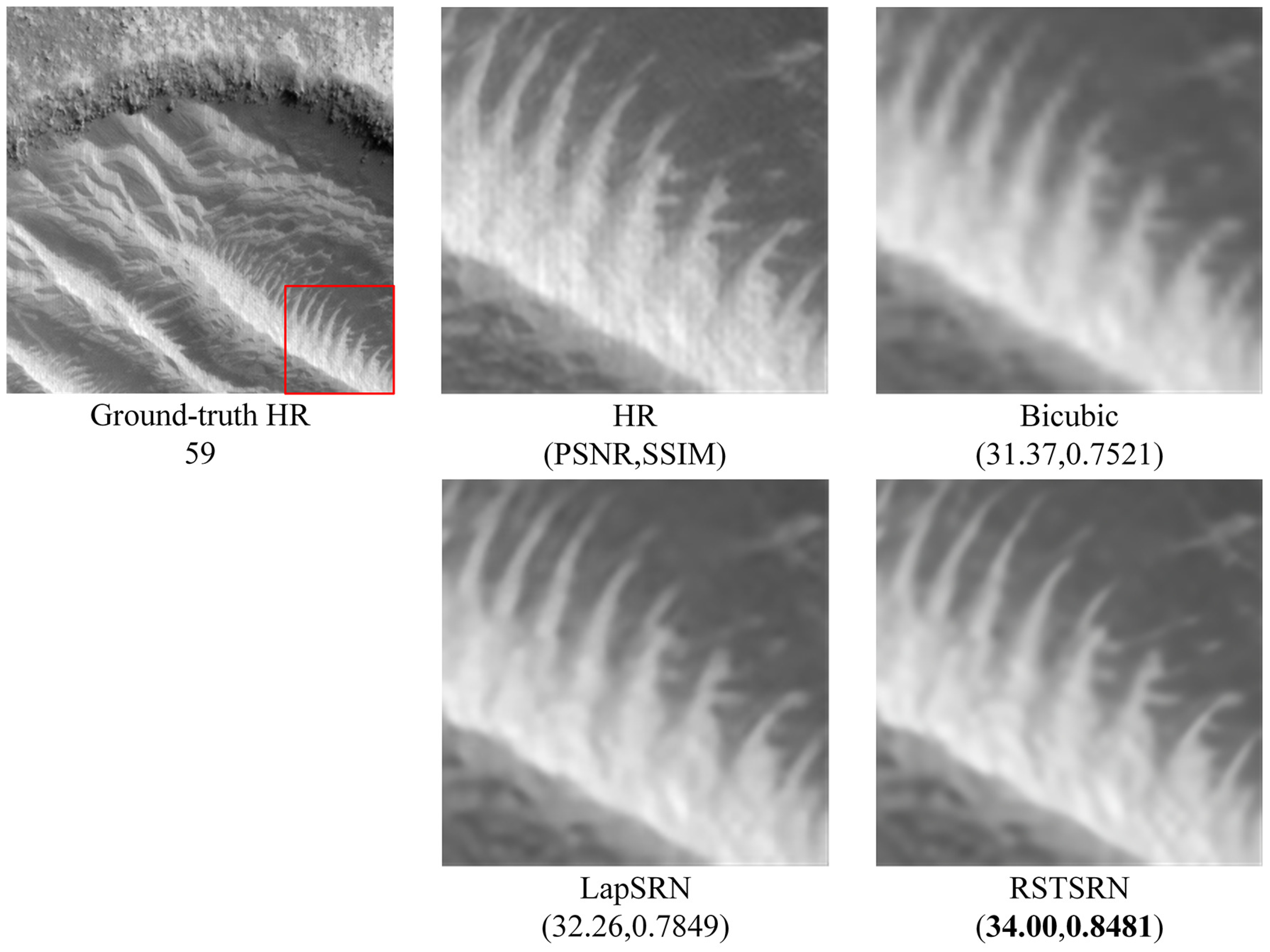
4.2. RSTSRN Results for Mars Image
5. Conclusions
Author Contributions
Funding
Institutional Review Board Statement
Informed Consent Statement
Data Availability Statement
Conflicts of Interest
Abbreviations
| AWSRN | Adaptive Weighted Super-Resolution Network |
| CARN | CAscading Residual Network |
| CNN | Convolutional Neural Network |
| DAT | Dual Aggregation Transformer |
| DEGREE | Deep Edge Guided REcurrent rEsidual |
| DIV2K | DIVerse 2K resolution image dataset |
| DiVANet | Directional Variance Attention Network |
| DRCN | Deeply Recursive Convolutional Network |
| DRRN | Deep Recursive Residual Network |
| D-DBPN | Dense Deep Back-Projection Networks |
| EDSR | Enhanced Deep Super-Resolution |
| ELAN | Efficient Long-range Attention Network |
| ESPCN | Efficient Sub-Pixel Convolutional neural Network |
| ESRT | Efficient Super-Resolution Transformer |
| FSRCNN | Fast Super-Resolution Convolutional Neural Network |
| HiRISE | High-Resolution Imaging Science Experiment |
| HNCT | Hybrid Network of CNN and Transformer |
| HR | High Resolution |
| IBP | Iterative Back-Projection |
| IMDN | Information Multi-Distillation Network |
| LapSRN | Laplacian pyramid Super-Resolution Network |
| LR | Low-Resolution |
| LRN | Laplacian Pyramid Recursive and Residual Network |
| MAP | Maximum A Posteriori |
| MemNet | Memory Network |
| MGS | Mars Global Surveyor |
| MISR | Multiple-Image Super-Resolution |
| MRO | Mars Reconnaissance Orbiter |
| MSRN | Multi-Scale Residual Network |
| NGswin | N-Gram Swin Transformer |
| POCS | Projection Onto Convex Sets |
| PSNR | Peak Signal-to-Noise Ratio |
| RDN | Residual Dense Network |
| RED-Net | very deep Residual Encoder–Decoder Networks |
| RFDN | Residual Feature Distillation Network |
| RIEB | Residual Image Extraction Block |
| RSTB | Residual Swin Transformer Block |
| RSTSRN | Recursive Swin Transformer Super-Resolution Network |
| SCN | Sparse-Coding-based Network |
| ScSR | Sparse-coding-based SR |
| SISR | Single-Image Super-Resolution |
| SPIN | Super Token Interaction Network |
| SR | Super-Resolution |
| SRCNN | Super-Resolution Convolutional Neural Network |
| SRDenseNet | Super-Resolution Dense convolutional Network |
| SRGAN | Super-Resolution Generative Adversarial Network |
| SSIM | Structural SIMilarity |
| STB | Swin Transformer Block |
| VDSR | Very Deep networks for Super-Resolution |
References
- Bell, J.F.; Squyres, S.W.; Arvidson, R.E.; Arneson, H.M.; Bass, D.; Blaney, D.; Cabrol, N.; Calvin, W.; Farmer, J.; Farrand, W.H.; et al. Pancam Multispectral Imaging Results from the Spirit Rover at Gusev Crater. Science 2004, 305, 800–806. [Google Scholar] [CrossRef]
- Bell, J.F.; Squyres, S.W.; Arvidson, R.E.; Arneson, H.M.; Bass, D.; Calvin, W.; Farrand, W.H.; Goetz, W.; Golombek, M.; Greeley, R.; et al. Pancam Multispectral Imaging Results from the Opportunity Rover at Meridiani Planum. Science 2004, 306, 1703–1709. [Google Scholar] [CrossRef]
- Blake, D.F.; Morris, R.V.; Kocurek, G.; Morrison, S.M.; Downs, R.T.; Bish, D.; Ming, D.W.; Edgett, K.S.; Rubin, D.; Goetz, W.; et al. Curiosity at Gale Crater, Mars: Characterization and Analysis of the Rocknest Sand Shadow. Science 2013, 341, 1239505. [Google Scholar] [CrossRef]
- Grotzinger, J.P.; Sumner, D.Y.; Kah, L.C.; Stack, K.; Gupta, S.; Edgar, L.; Rubin, D.; Lewis, K.; Schieber, J.; Mangold, N.; et al. A Habitable Fluvio-Lacustrine Environment at Yellowknife Bay, Gale Crater, Mars. Science 2014, 343, 1242777. [Google Scholar] [CrossRef]
- McEwen, A.S.; Eliason, E.M.; Bergstrom, J.W.; Bridges, N.T.; Hansen, C.J.; Delamere, W.A.; Grant, J.A.; Gulick, V.C.; Herkenhoff, K.E.; Keszthelyi, L.; et al. Mars Reconnaissance Orbiter’s High Resolution Imaging Science Experiment (HiRISE). J. Geophys. Res. Planets 2007, 112, E05S02. [Google Scholar] [CrossRef]
- Kirk, R.L.; Howington-Kraus, E.; Rosiek, M.R.; Anderson, J.A.; Archinal, B.A.; Becker, K.J.; Cook, D.A.; Galuszka, D.M.; Geissler, P.E.; Hare, T.M.; et al. Ultrahigh resolution topographic mapping of Mars with MRO HiRISE stereo images: Meter-scale slopes of candidate Phoenix landing sites. J. Geophys. Res. Planets 2008, 113, E00A24. [Google Scholar] [CrossRef]
- Keszthelyi, L.; Jaeger, W.; McEwen, A.; Tornabene, L.; Beyer, R.A.; Dundas, C.; Milazzo, M. High Resolution Imaging Science Experiment (HiRISE) images of volcanic terrains from the first 6 months of the Mars Reconnaissance Orbiter Primary Science Phase. J. Geophys. Res. Planets 2008, 113, E04005. [Google Scholar] [CrossRef]
- Lefort, A.; Russell, P.S.; Thomas, N.; McEwen, A.S.; Dundas, C.M.; Kirk, R.L. Observations of periglacial landforms in Utopia Planitia with the High Resolution Imaging Science Experiment (HiRISE). J. Geophys. Res. Planets 2009, 114, E04005. [Google Scholar] [CrossRef]
- Dundas, C.M.; McEwen, A.S.; Diniega, S.; Byrne, S.; Martinez-Alonso, S. New and recent gully activity on Mars as seen by HiRISE. Geophys. Res. Lett. 2010, 37, L07202. [Google Scholar] [CrossRef]
- Lai, W.S.; Huang, J.B.; Ahuja, N.; Yang, M.H. Deep Laplacian Pyramid Networks for Fast and Accurate Super-Resolution. In Proceedings of the 2017 IEEE Conference on Computer Vision and Pattern Recognition (CVPR), Honolulu, HI, USA, 21–26 July 2017; pp. 5835–5843. [Google Scholar] [CrossRef]
- Wu, F.L.; Wang, X.J. Example-based super-resolution for single-image analysis from the Chang’e-1 Mission. Res. Astron. Astrophys. 2016, 16, 172. [Google Scholar] [CrossRef]
- Zhang, H.; Yang, Z.; Zhang, L.; Shen, H. Super-Resolution Reconstruction for Multi-Angle Remote Sensing Images Considering Resolution Differences. Remote Sens. 2014, 6, 637–657. [Google Scholar] [CrossRef]
- Tao, Y.; Muller, J.P. Super-Resolution Restoration of MISR Images Using the UCL MAGiGAN System. Remote Sens. 2019, 11, 52. [Google Scholar] [CrossRef]
- Ma, J.; Zhang, L.; Zhang, J. SD-GAN: Saliency-Discriminated GAN for Remote Sensing Image Superresolution. IEEE Geosci. Remote Sens. Lett. 2020, 17, 1973–1977. [Google Scholar] [CrossRef]
- Yu, Y.; Li, X.; Liu, F. E-DBPN: Enhanced Deep Back-Projection Networks for Remote Sensing Scene Image Superresolution. IEEE Trans. Geosci. Remote Sens. 2020, 58, 5503–5515. [Google Scholar] [CrossRef]
- Wang, Y.H.; Qiao, J.; Li, J.B.; Fu, P.; Chu, S.C.; Roddick, J.F. Sparse representation-based MRI super-resolution reconstruction. Measurement 2014, 47, 946–953. [Google Scholar] [CrossRef]
- Lyu, Q.; Shan, H.; Steber, C.; Helis, C.; Whitlow, C.; Chan, M.; Wang, G. Multi-Contrast Super-Resolution MRI through a Progressive Network. IEEE Trans. Med Imaging 2020, 39, 2738–2749. [Google Scholar] [CrossRef]
- Wu, Z.; Chen, X.; Xie, S.; Shen, J.; Zeng, Y. Super-resolution of brain MRI images based on denoising diffusion probabilistic model. Biomed. Signal Process. Control 2023, 85, 104901. [Google Scholar] [CrossRef]
- Gunturk, B.; Batur, A.; Altunbasak, Y.; Hayes, M.; Mersereau, R. Eigenface-domain super-resolution for face recognition. IEEE Trans. Image Process. 2003, 12, 597–606. [Google Scholar] [CrossRef]
- Grm, K.; Scheirer, W.J.; Struc, V. Face Hallucination Using Cascaded Super-Resolution and Identity Priors. IEEE Trans. Image Process. 2020, 29, 2150–2165. [Google Scholar] [CrossRef]
- Hou, H.; Xu, J.; Hou, Y.; Hu, X.; Wei, B.; Shen, D. Semi-Cycled Generative Adversarial Networks for Real-World Face Super-Resolution. IEEE Trans. Image Process. 2023, 32, 1184–1199. [Google Scholar] [CrossRef]
- Hardie, R.; Barnard, K.; Armstrong, E. Joint MAP registration and high-resolution image estimation using a sequence of undersampled images. IEEE Trans. Image Process. 1997, 6, 1621–1633. [Google Scholar] [CrossRef]
- Farsiu, S.; Robinson, M.; Elad, M.; Milanfar, P. Fast and Robust Multiframe Super Resolution. IEEE Trans. Image Process. 2004, 13, 1327–1344. [Google Scholar] [CrossRef]
- Yuan, Q.; Zhang, L.; Shen, H. Multiframe Super-Resolution Employing a Spatially Weighted Total Variation Model. IEEE Trans. Circuits Syst. Video Technol. 2012, 22, 379–392. [Google Scholar] [CrossRef]
- Freeman, W.; Jones, T.; Pasztor, E. Example-based super-resolution. IEEE Comput. Graph. Appl. 2002, 22, 56–65. [Google Scholar] [CrossRef]
- Wang, Z.; Chen, J.; Hoi, S.C.H. Deep Learning for Image Super-Resolution: A Survey. IEEE Trans. Pattern Anal. Mach. Intell. 2021, 43, 3365–3387. [Google Scholar] [CrossRef]
- Tao, Y.; Conway, S.J.; Muller, J.P.; Putri, A.R.D.; Thomas, N.; Cremonese, G. Single Image Super-Resolution Restoration of TGO CaSSIS Colour Images: Demonstration with Perseverance Rover Landing Site and Mars Science Targets. Remote Sens. 2021, 13, 1777. [Google Scholar] [CrossRef]
- Stark, H.; Oskoui, P. High-resolution image recovery from image-plane arrays, using convex projections. J. Opt. Soc. Am. A 1989, 6, 1715–1726. [Google Scholar] [CrossRef]
- Patti, A.; Sezan, M.; Tekalp, A.M. Superresolution video reconstruction with arbitrary sampling lattices and nonzero aperture time. IEEE Trans. Image Process. 1997, 6, 1064–1076. [Google Scholar] [CrossRef]
- Patti, A.; Altunbasak, Y. Artifact reduction for set theoretic super resolution image reconstruction with edge adaptive constraints and higher-order interpolants. IEEE Trans. Image Process. 2001, 10, 179–186. [Google Scholar] [CrossRef]
- Irani, M.; Peleg, S. Improving resolution by image registration. CVGIP Graph. Model. Image Process. 1991, 53, 231–239. [Google Scholar] [CrossRef]
- Irani, M.; Peleg, S. Motion Analysis for Image Enhancement: Resolution, Occlusion, and Transparency. J. Vis. Commun. Image Represent. 1993, 4, 324–335. [Google Scholar] [CrossRef]
- Schultz, R.; Stevenson, R. A Bayesian approach to image expansion for improved definition. IEEE Trans. Image Process. 1994, 3, 233–242. [Google Scholar] [CrossRef] [PubMed]
- Schultz, R.; Stevenson, R. Extraction of high-resolution frames from video sequences. IEEE Trans. Image Process. 1996, 5, 996–1011. [Google Scholar] [CrossRef] [PubMed]
- Shen, H.; Zhang, L.; Huang, B.; Li, P. A MAP Approach for Joint Motion Estimation, Segmentation, and Super Resolution. IEEE Trans. Image Process. 2007, 16, 479–490. [Google Scholar] [CrossRef]
- Belekos, S.P.; Galatsanos, N.P.; Katsaggelos, A.K. Maximum a Posteriori Video Super-Resolution Using a New Multichannel Image Prior. IEEE Trans. Image Process. 2010, 19, 1451–1464. [Google Scholar] [CrossRef]
- Elad, M.; Feuer, A. Restoration of a single superresolution image from several blurred, noisy, and undersampled measured images. IEEE Trans. Image Process. 1997, 6, 1646–1658. [Google Scholar] [CrossRef]
- Yang, J.; Wright, J.; Huang, T.S.; Ma, Y. Image Super-Resolution Via Sparse Representation. IEEE Trans. Image Process. 2010, 19, 2861–2873. [Google Scholar] [CrossRef]
- Tao, Y.; Xiong, S.; Song, R.; Muller, J.P. Towards Streamlined Single-Image Super-Resolution: Demonstration with 10 m Sentinel-2 Colour and 10–60 m Multi-Spectral VNIR and SWIR Bands. Remote Sens. 2021, 13, 2614. [Google Scholar] [CrossRef]
- Tao, Y.; Xiong, S.; Muller, J.P.; Michael, G.; Conway, S.J.; Paar, G.; Cremonese, G.; Thomas, N. Subpixel-Scale Topography Retrieval of Mars Using Single-Image DTM Estimation and Super-Resolution Restoration. Remote Sens. 2022, 14, 257. [Google Scholar] [CrossRef]
- Zou, H.; He, S.; Cao, X.; Sun, L.; Wei, J.; Liu, S.; Liu, J. Rescaling-Assisted Super-Resolution for Medium-Low Resolution Remote Sensing Ship Detection. Remote Sens. 2022, 14, 2566. [Google Scholar] [CrossRef]
- Dong, C.; Loy, C.C.; He, K.; Tang, X. Image Super-Resolution Using Deep Convolutional Networks. IEEE Trans. Pattern Anal. Mach. Intell. 2016, 38, 295–307. [Google Scholar] [CrossRef]
- Dong, C.; Loy, C.C.; Tang, X. Accelerating the Super-Resolution Convolutional Neural Network. In Computer Vision—ECCV 2016; Springer International Publishing: Cham, Switzerland, 2016; pp. 391–407. [Google Scholar] [CrossRef]
- Shi, W.; Caballero, J.; Huszar, F.; Totz, J.; Aitken, A.P.; Bishop, R.; Rueckert, D.; Wang, Z. Real-Time Single Image and Video Super-Resolution Using an Efficient Sub-Pixel Convolutional Neural Network. In Proceedings of the 2016 IEEE Conference on Computer Vision and Pattern Recognition (CVPR), Las Vegas, NV, USA, 27–30 June 2016; pp. 1874–1883. [Google Scholar] [CrossRef]
- Kim, J.; Lee, J.K.; Lee, K.M. Accurate Image Super-Resolution Using Very Deep Convolutional Networks. In Proceedings of the 2016 IEEE Conference on Computer Vision and Pattern Recognition (CVPR), Las Vegas, NV, USA, 27–30 June 2016; pp. 1646–1654. [Google Scholar] [CrossRef]
- Kim, J.; Lee, J.K.; Lee, K.M. Deeply-Recursive Convolutional Network for Image Super-Resolution. In Proceedings of the 2016 IEEE Conference on Computer Vision and Pattern Recognition (CVPR), Las Vegas, NV, USA, 27–30 June 2016; pp. 1637–1645. [Google Scholar] [CrossRef]
- Wang, Z.; Liu, D.; Yang, J.; Han, W.; Huang, T. Deep Networks for Image Super-Resolution with Sparse Prior. In Proceedings of the 2015 IEEE International Conference on Computer Vision (ICCV), Santiago, Chile, 7–13 December 2015; pp. 370–378. [Google Scholar] [CrossRef]
- Yang, W.; Feng, J.; Yang, J.; Zhao, F.; Liu, J.; Guo, Z.; Yan, S. Deep Edge Guided Recurrent Residual Learning for Image Super-Resolution. IEEE Trans. Image Process. 2017, 26, 5895–5907. [Google Scholar] [CrossRef]
- Tai, Y.; Yang, J.; Liu, X.; Xu, C. MemNet: A Persistent Memory Network for Image Restoration. In Proceedings of the 2017 IEEE International Conference on Computer Vision (ICCV), Venice, Italy, 22–29 October 2017; pp. 4549–4557. [Google Scholar] [CrossRef]
- Tai, Y.; Yang, J.; Liu, X. Image Super-Resolution via Deep Recursive Residual Network. In Proceedings of the 2017 IEEE Conference on Computer Vision and Pattern Recognition (CVPR), Honolulu, HI, USA, 21–26 July 2017; pp. 2790–2798. [Google Scholar] [CrossRef]
- Tong, T.; Li, G.; Liu, X.; Gao, Q. Image Super-Resolution Using Dense Skip Connections. In Proceedings of the 2017 IEEE International Conference on Computer Vision (ICCV), Venice, Italy, 22–29 October 2017; pp. 4809–4817. [Google Scholar] [CrossRef]
- Ledig, C.; Theis, L.; Huszar, F.; Caballero, J.; Cunningham, A.; Acosta, A.; Aitken, A.; Tejani, A.; Totz, J.; Wang, Z.; et al. Photo-Realistic Single Image Super-Resolution Using a Generative Adversarial Network. In Proceedings of the 2017 IEEE Conference on Computer Vision and Pattern Recognition (CVPR), Honolulu, HI, USA, 21–26 July 2017; pp. 105–114. [Google Scholar] [CrossRef]
- Zhang, Y.; Tian, Y.; Kong, Y.; Zhong, B.; Fu, Y. Residual Dense Network for Image Super-Resolution. In Proceedings of the 2018 IEEE/CVF Conference on Computer Vision and Pattern Recognition, Salt Lake City, UT, USA, 18–23 June 2018; pp. 2472–2481. [Google Scholar] [CrossRef]
- Liang, J.; Cao, J.; Sun, G.; Zhang, K.; Gool, L.V.; Timofte, R. SwinIR: Image Restoration Using Swin Transformer. arXiv 2021, arXiv:2108.10257. [Google Scholar] [CrossRef]
- Choi, H.; Lee, J.; Yang, J. N-Gram in Swin Transformers for Efficient Lightweight Image Super-Resolution. In Proceedings of the 2023 IEEE/CVF Conference on Computer Vision and Pattern Recognition (CVPR), Vancouver, BC, Canada, 17–24 June 2023; pp. 2071–2081. [Google Scholar] [CrossRef]
- Chen, Z.; Zhang, Y.; Gu, J.; Kong, L.; Yang, X.; Yu, F. Dual Aggregation Transformer for Image Super-Resolution. In Proceedings of the 2023 IEEE/CVF International Conference on Computer Vision (ICCV), Paris, France, 1–6 October 2023; pp. 12278–12287. [Google Scholar] [CrossRef]
- Tao, Y.; Douté, S.; Muller, J.P.; Conway, S.J.; Thomas, N.; Cremonese, G. Ultra-High-Resolution 1 m/pixel CaSSIS DTM Using Super-Resolution Restoration and Shape-from-Shading: Demonstration over Oxia Planum on Mars. Remote Sens. 2021, 13, 2185. [Google Scholar] [CrossRef]
- Tao, Y.; Muller, J.P. Super-Resolution Restoration of Spaceborne Ultra-High-Resolution Images Using the UCL OpTiGAN System. Remote Sens. 2021, 13, 2269. [Google Scholar] [CrossRef]
- Delgado-Centeno, J.I.; Sanchez-Cuevas, P.J.; Martinez, C.; Olivares-Mendez, M. Enhancing Lunar Reconnaissance Orbiter Images via Multi-Frame Super Resolution for Future Robotic Space Missions. IEEE Robot. Autom. Lett. 2021, 6, 7721–7727. [Google Scholar] [CrossRef]
- Wang, C.; Zhang, Y.; Zhang, Y.; Tian, R.; Ding, M. Mars Image Super-Resolution Based on Generative Adversarial Network. IEEE Access 2021, 9, 108889–108898. [Google Scholar] [CrossRef]
- Tewari, A.; Prateek, C.; Khanna, N. In-Orbit Lunar Satellite Image Super Resolution for Selective Data Transmission. arXiv 2021, arXiv:2110.10109. [Google Scholar] [CrossRef]
- Zhang, N.; Wang, Y.; Zhang, X.; Xu, D.; Wang, X. An Unsupervised Remote Sensing Single-Image Super-Resolution Method Based on Generative Adversarial Network. IEEE Access 2020, 8, 29027–29039. [Google Scholar] [CrossRef]
- Zhang, N.; Wang, Y.; Zhang, X.; Xu, D.; Wang, X.; Ben, G.; Zhao, Z.; Li, Z. A Multi-Degradation Aided Method for Unsupervised Remote Sensing Image Super Resolution With Convolution Neural Networks. IEEE Trans. Geosci. Remote Sens. 2022, 60, 5600814. [Google Scholar] [CrossRef]
- Geng, M.; Wu, F.; Wang, D. Lightweight Mars remote sensing image super-resolution reconstruction network. Opt. Precis. Eng. 2022, 30, 1487–1498. [Google Scholar] [CrossRef]
- Liu, Z.; Lin, Y.; Cao, Y.; Hu, H.; Wei, Y.; Zhang, Z.; Lin, S.; Guo, B. Swin Transformer: Hierarchical Vision Transformer using Shifted Windows. arXiv 2021, arXiv:2103.14030. [Google Scholar] [CrossRef]
- Agustsson, E.; Timofte, R. NTIRE 2017 Challenge on Single Image Super-Resolution: Dataset and Study. In Proceedings of the 2017 IEEE Conference on Computer Vision and Pattern Recognition Workshops (CVPRW), Honolulu, HI, USA, 21–26 July 2017; pp. 1122–1131. [Google Scholar] [CrossRef]
- Bevilacqua, M.; Roumy, A.; Guillemot, C.; Alberi Morel, M.-L. Low-Complexity Single-Image Super-Resolution based on Nonnegative Neighbor Embedding. In Proceedings of the British Machine Vision Conference 2012, Surrey, UK, 3–7 September 2012; pp. 135.1–135.10. [Google Scholar] [CrossRef]
- Zeyde, R.; Elad, M.; Protter, M. On Single Image Scale-Up Using Sparse-Representations. In Curves and Surfaces; Springer: Berlin/Heidelberg, Germany, 2012; pp. 711–730. [Google Scholar] [CrossRef]
- Arbeláez, P.; Maire, M.; Fowlkes, C.; Malik, J. Contour Detection and Hierarchical Image Segmentation. IEEE Trans. Pattern Anal. Mach. Intell. 2011, 33, 898–916. [Google Scholar] [CrossRef]
- Huang, J.B.; Singh, A.; Ahuja, N. Single image super-resolution from transformed self-exemplars. In Proceedings of the 2015 IEEE Conference on Computer Vision and Pattern Recognition (CVPR), Boston, MA, USA, 7–12 June 2015; pp. 5197–5206. [Google Scholar] [CrossRef]
- Matsui, Y.; Ito, K.; Aramaki, Y.; Fujimoto, A.; Ogawa, T.; Yamasaki, T.; Aizawa, K. Sketch-based manga retrieval using manga109 dataset. Multimed. Tools Appl. 2017, 76, 21811–21838. [Google Scholar] [CrossRef]
- Lim, B.; Son, S.; Kim, H.; Nah, S.; Lee, K.M. Enhanced Deep Residual Networks for Single Image Super-Resolution. In Proceedings of the 2017 IEEE Conference on Computer Vision and Pattern Recognition Workshops (CVPRW), Honolulu, HI, USA, 21–26 July 2017; pp. 1132–1140. [Google Scholar] [CrossRef]
- Ahn, N.; Kang, B.; Sohn, K.A. Fast, Accurate, and Lightweight Super-Resolution with Cascading Residual Network. In Computer Vision—ECCV 2018; Springer International Publishing: Cham, Switzerland, 2018; pp. 256–272. [Google Scholar] [CrossRef]
- Haris, M.; Shakhnarovich, G.; Ukita, N. Deep Back-Projection Networks for Super-Resolution. In Proceedings of the 2018 IEEE/CVF Conference on Computer Vision and Pattern Recognition, Salt Lake City, UT, USA, 18–23 June 2018; pp. 1664–1673. [Google Scholar] [CrossRef]
- Li, J.; Fang, F.; Mei, K.; Zhang, G. Multi-scale Residual Network for Image Super-Resolution. In Computer Vision—ECCV 2018; Springer International Publishing: Cham, Switzerland, 2018; pp. 527–542. [Google Scholar] [CrossRef]
- Hui, Z.; Gao, X.; Yang, Y.; Wang, X. Lightweight Image Super-Resolution with Information Multi-distillation Network. In Proceedings of the Proceedings of the 27th ACM International Conference on Multimedia, Nice, France, 21–25 October 2019; pp. 2024–2032. [Google Scholar] [CrossRef]
- Wang, C.; Li, Z.; Shi, J. Lightweight Image Super-Resolution with Adaptive Weighted Learning Network. arXiv 2019, arXiv:1904.02358. [Google Scholar] [CrossRef]
- Liu, J.; Tang, J.; Wu, G. Residual Feature Distillation Network for Lightweight Image Super-Resolution. In Computer Vision—ECCV 2020 Workshops; Springer International Publishing: Cham, Switzerland, 2020; pp. 41–55. [Google Scholar] [CrossRef]
- Luo, X.; Xie, Y.; Zhang, Y.; Qu, Y.; Li, C.; Fu, Y. LatticeNet: Towards Lightweight Image Super-Resolution with Lat-tice Block. In Computer Vision—ECCV 2020; Springer International Publishing: Cham, Switzerland, 2020; pp. 272–289. [Google Scholar] [CrossRef]
- Fang, J.; Lin, H.; Chen, X.; Zeng, K. A Hybrid Network of CNN and Transformer for Lightweight Image Super-Resolution. In Proceedings of the 2022 IEEE/CVF Conference on Computer Vision and Pattern Recognition Workshops (CVPRW), New Orleans, LA, USA, 19–20 June 2022; pp. 1102–1111. [Google Scholar] [CrossRef]
- Zhang, X.; Zeng, H.; Guo, S.; Zhang, L. Efficient Long-Range Attention Network for Image Super-Resolution. In Computer Vision—ECCV 2022; Springer Nature: Cham, Switzerland, 2022; pp. 649–667. [Google Scholar] [CrossRef]
- Lu, Z.; Li, J.; Liu, H.; Huang, C.; Zhang, L.; Zeng, T. Transformer for Single Image Super-Resolution. In Proceedings of the 2022 IEEE/CVF Conference on Computer Vision and Pattern Recognition Workshops (CVPRW), New Orleans, LA, USA, 19–20 June 2022; pp. 456–465. [Google Scholar] [CrossRef]
- Zhang, A.; Ren, W.; Liu, Y.; Cao, X. Lightweight Image Super-Resolution with Superpixel Token Interaction. In Proceedings of the 2023 IEEE/CVF International Conference on Computer Vision (ICCV), Paris, France, 1–6 October 2023; pp. 12682–12691. [Google Scholar] [CrossRef]
- Behjati, P.; Rodriguez, P.; Fernández, C.; Hupont, I.; Mehri, A.; Gonzàlez, J. Single image super-resolution based on directional variance attention network. Pattern Recognit. 2023, 133, 108997. [Google Scholar] [CrossRef]
- Wang, Z.; Bovik, A.; Sheikh, H.; Simoncelli, E. Image Quality Assessment: From Error Visibility to Structural Similarity. IEEE Trans. Image Process. 2004, 13, 600–612. [Google Scholar] [CrossRef]


| Algorithm | Scale | Year | Parameters | Set5 PSNR/SSIM | Set14 PSNR/SSIM | BSDS100 PSNR/SSIM | Urban100 PSNR/SSIM | MANGA109 PSNR/SSIM |
|---|---|---|---|---|---|---|---|---|
| Bicubic | 2× | - | - | 33.66/0.9284 | 30.34/0.8675 | 29.57/0.8434 | 26.88/0.8438 | 30.82/0.9332 |
| VDSR [45] | 2× | 2016 | 665K | 37.53/0.9587 | 33.03/0.9124 | 31.90/0.8960 | 30.76/0.9140 | 37.22/0.9729 |
| DRCN [46] | 2× | 2016 | 1774K | 37.63/0.9588 | 33.04/0.9118 | 31.85/0.8942 | 30.75/0.9133 | 37.63/0.9723 |
| MemNet [49] | 2× | 2017 | 677K | 37.78/0.9597 | 33.28/0.9142 | 32.08/0.8978 | 31.31/0.9195 | 37.72/0.9740 |
| LapSRN [10] | 2× | 2017 | 813K | 37.52/0.9581 | 33.08/0.9109 | 31.80/0.8949 | 30.41/0.9112 | 37.27/0.9745 |
| EDSR [72] | 2× | 2017 | 43000K | 38.11/0.9601 | 33.92/0.9195 | 32.32/0.9013 | 32.93/0.9351 | 39.10/0.9773 |
| CARN [73] | 2× | 2018 | 1592K | 37.76/0.9590 | 33.52/0.9166 | 32.09/0.8978 | 31.51/0.9312 | 38.36/0.9764 |
| D-DBPN [74] | 2× | 2018 | 5819K | 38.09/0.9600 | 33.85/0.9190 | 32.27/0.9000 | 32.55/0.9324 | 38.89/0.9775 |
| MSRN [75] | 2× | 2018 | 5930K | 38.08/0.9605 | 33.74/0.9170 | 32.23/0.9013 | 32.22/0.9326 | 38.69/0.9772 |
| IMDN [76] | 2× | 2019 | 694K | 38.00/0.9605 | 33.63/0.9177 | 32.19/0.8996 | 32.17/0.9283 | 38.88/0.9774 |
| AWSRN [77] | 2× | 2019 | 1397K | 38.11/0.9608 | 33.78/0.9189 | 32.26/0.9006 | 32.49/0.9316 | 38.87/0.9776 |
| RFDN-L [78] | 2× | 2020 | 626K | 38.08/0.9606 | 33.67/0.9190 | 32.18/0.8996 | 32.24/0.9290 | 38.95/0.9773 |
| LatticeNet [79] | 2× | 2020 | 756K | 38.15/0.9610 | 33.78/0.9193 | 32.25/0.9005 | 32.43/0.9302 | - |
| HNCT [80] | 2× | 2022 | 356K | 38.08/0.9608 | 33.65/0.9182 | 32.22/0.9001 | 32.22/0.9294 | 38.87/0.9774 |
| ELAN-light [81] | 2× | 2022 | 582K | 38.17/0.9611 | 33.94/0.9207 | 32.30/0.9012 | 32.76/0.9340 | 39.11/0.9782 |
| ESRT [82] | 2× | 2022 | 677K | 38.03/0.9600 | 33.75/0.9184 | 32.25/0.9001 | 32.58/0.9318 | 39.12/0.9783 |
| SPIN [83] | 2× | 2023 | 497K | 38.20/0.9615 | 33.90/0.9215 | 32.31/0.9015 | 32.79/0.9340 | 39.18/0.9784 |
| DiVANet [84] | 2× | 2023 | 902K | 38.16/0.9612 | 33.80/0.9195 | 32.29/0.9012 | 32.60/0.9325 | 39.08/0.9775 |
| NGswin [55] | 2× | 2023 | 998K | 38.05/0.9610 | 33.79/0.9199 | 32.27/0.9008 | 32.53/0.9324 | 38.97/0.9777 |
| RSTSRN (ours) | 2× | - | 1830K | 38.11/0.9619 | 33.92/0.9209 | 32.30/0.9012 | 32.68/0.9340 | 39.04/0.9779 |
| Bicubic | 4× | - | - | 28.43/0.8022 | 26.10/0.6936 | 25.97/0.6517 | 23.14/0.6599 | 24.91/0.7826 |
| VDSR [45] | 4× | 2016 | 665K | 31.35/0.8838 | 28.01/0.7674 | 27.29/0.7251 | 25.18/0.7524 | 28.83/0.8809 |
| DRCN [46] | 4× | 2016 | 1774K | 31.53/0.8840 | 28.04/0.7700 | 27.24/0.7240 | 25.14/0.7520 | 28.97/0.8860 |
| MemNet [49] | 4× | 2017 | 677K | 31.74/0.8893 | 28.26/0.7723 | 27.40/0.7281 | 25.50/0.7630 | 29.42/0.8942 |
| LapSRN [10] | 4× | 2017 | 813K | 31.54/0.8856 | 28.19/0.7720 | 27.32/0.7280 | 25.21/0.7560 | 29.09/0.8900 |
| EDSR [72] | 4× | 2017 | 43000K | 32.46/0.8968 | 28.80/0.7876 | 27.71/0.7420 | 26.64/0.8033 | 31.02/0.9148 |
| CARN [73] | 4× | 2018 | 1592K | 32.13/0.8937 | 28.60/0.7806 | 27.58/0.7349 | 26.07/0.7837 | 30.36/0.9082 |
| D-DBPN [74] | 4× | 2018 | 10291K | 32.47/0.8970 | 28.82/0.7860 | 27.72/0.7400 | 26.38/0.7946 | 30.91/0.9137 |
| MSRN [75] | 4× | 2018 | 6078K | 32.07/0.8903 | 28.60/0.7751 | 27.52/0.7273 | 26.04/0.7896 | 30.17/0.9034 |
| IMDN [76] | 4× | 2019 | 715K | 32.21/0.8948 | 28.58/0.7811 | 27.56/0.7353 | 26.04/0.7838 | 30.45/0.9075 |
| AWSRN [77] | 4× | 2019 | 1587K | 32.27/0.8960 | 28.69/0.7843 | 27.64/0.7385 | 26.29/0.7930 | 30.72/0.9109 |
| RFDN-L [78] | 4× | 2020 | 643K | 32.28/0.8957 | 28.61/0.7818 | 27.58/0.7363 | 26.20/0.7883 | 30.61/0.9096 |
| LatticeNet [79] | 4× | 2020 | 777K | 32.30/0.8962 | 28.68/0.7830 | 27.62/0.7367 | 26.25/0.7873 | - |
| HNCT [80] | 4× | 2022 | 372K | 32.31/0.8957 | 28.71/0.7834 | 27.63/0.7381 | 26.20/0.7896 | 30.70/0.9112 |
| ELAN-light [81] | 4× | 2022 | 601K | 32.43/0.8975 | 28.78/0.7858 | 27.69/0.7406 | 26.54/0.7982 | 30.92/0.9150 |
| ESRT [82] | 4× | 2022 | 751K | 32.19/0.8947 | 28.69/0.7833 | 27.69/0.7379 | 26.39/0.7962 | 30.75/0.9100 |
| SPIN [83] | 4× | 2023 | 555K | 32.48/0.8983 | 28.80/0.7862 | 27.70/0.7415 | 26.55/0.7998 | 30.98/0.9156 |
| DiVANet [84] | 4× | 2023 | 939K | 32.41/0.8973 | 28.70/0.7844 | 27.65/0.7391 | 26.42/0.7958 | 30.73/0.9119 |
| NGswin [55] | 4× | 2023 | 1019K | 32.33/0.8963 | 28.78/0.7859 | 27.66/0.7396 | 26.45/0.7963 | 30.80/0.9128 |
| RSTSRN (ours) | 4× | - | 1830K | 32.63/0.9008 | 28.89/0.7895 | 27.77/0.7435 | 26.78/0.8075 | 31.40/0.9192 |
| Bicubic | 8× | - | - | 24.40/0.6045 | 23.19/0.5110 | 23.67/0.4808 | 20.74/0.4841 | 21.46/0.6138 |
| VDSR [45] | 8× | 2016 | 665K | 25.73/0.6743 | 23.20/0.5110 | 24.34/0.5169 | 21.48/0.5289 | 22.73/0.6688 |
| DRCN [46] | 8× | 2016 | 1774K | 25.93/0.6743 | 24.25/0.5510 | 24.49/0.5168 | 21.71/0.5289 | 23.20/0.6686 |
| MemNet [49] | - | 2017 | - | - | - | - | - | - |
| LapSRN [10] | 8× | 2017 | 813K | 26.15/0.7028 | 24.45/0.5792 | 24.54/0.5293 | 21.81/0.5555 | 23.39/0.7068 |
| EDSR [72] | 8× | 2017 | 43000K | 26.96/0.7762 | 24.91/0.6420 | 24.81/0.5985 | 22.51/0.6221 | 24.69/0.7841 |
| CARN [73] | - | 2018 | - | - | - | - | - | - |
| D-DBPN [74] | 8× | 2018 | 23071K | 27.21/0.7840 | 25.13/0.6480 | 24.88/0.6010 | 22.73/0.6312 | 25.14/0.7987 |
| MSRN [75] | 8× | 2018 | 6226K | 26.59/0.7254 | 24.88/0.5961 | 24.70/0.5410 | 22.37/0.5977 | 24.28/0.7517 |
| IMDN [76] | - | 2019 | - | - | - | - | - | - |
| AWSRN [77] | 8× | 2019 | 2348K | 26.97/0.7747 | 24.99/0.6414 | 24.80/0.5967 | 22.45/0.6174 | 24.60/0.7782 |
| RFDN-L [78] | - | 2020 | - | - | - | - | - | - |
| LatticeNet [79] | - | 2020 | - | - | - | - | - | - |
| HNCT [80] | - | 2022 | - | - | - | - | - | - |
| ELAN-light [81] | - | 2022 | - | - | - | - | - | - |
| ESRT [82] | - | 2022 | - | - | - | - | - | - |
| SPIN [83] | - | 2023 | - | - | - | - | - | - |
| DiVANet [84] | - | 2023 | - | - | - | - | - | - |
| NGswin [55] | - | 2023 | - | - | - | - | - | - |
| RSTSRN (ours) | 8× | - | 1830K | 27.30/0.7895 | 25.24/0.6498 | 24.96/0.6045 | 23.02/0.6458 | 25.23/0.8022 |
| Method | Year | 2× | 4× | 8× | Multi-Scales |
|---|---|---|---|---|---|
| VDSR [45] | 2016 | 665 K | 665 K | 665 K | 1995 K |
| DRCN [46] | 2016 | 1774 K | 1774 K | 1774 K | 5322 K |
| MemNet [49] | 2017 | 677 K | 677 K | - | 1354 K |
| LapSRN [10] | 2017 | 813 K | 813 K | 813 K | 2439 K |
| CARN [73] | 2018 | 1592 K | 1592 K | - | 3184 K |
| AWSRN [77] | 2019 | 1397 K | 1587 K | 2348 K | 5332 K |
| RSTSRN(ours) | - | 1830 K | 1830 K | 1830 K | 1830 K |
| Method | Scale | PSNR/dB | SSIM |
|---|---|---|---|
| Bicubic | 2× | 34.09 | 0.8228 |
| LapSRN [10] | 2× | 34.72 | 0.8477 |
| RSTSRN(ours) | 2× | 35.07 | 0.8525 |
| Bicubic | 4× | 31.31 | 0.7124 |
| LapSRN [10] | 4× | 31.94 | 0.7396 |
| RSTSRN(ours) | 4× | 32.82 | 0.7510 |
| Bicubic | 8× | 28.60 | 0.6128 |
| LapSRN [10] | 8× | 29.23 | 0.6327 |
| RSTSRN(ours) | 8× | 30.45 | 0.6638 |
Disclaimer/Publisher’s Note: The statements, opinions and data contained in all publications are solely those of the individual author(s) and contributor(s) and not of MDPI and/or the editor(s). MDPI and/or the editor(s) disclaim responsibility for any injury to people or property resulting from any ideas, methods, instructions or products referred to in the content. |
© 2024 by the authors. Licensee MDPI, Basel, Switzerland. This article is an open access article distributed under the terms and conditions of the Creative Commons Attribution (CC BY) license (https://creativecommons.org/licenses/by/4.0/).
Share and Cite
Wu, F.; Jiang, X.; Fu, T.; Fu, Y.; Xu, D.; Zhao, C. RSTSRN: Recursive Swin Transformer Super-Resolution Network for Mars Images. Appl. Sci. 2024, 14, 9286. https://doi.org/10.3390/app14209286
Wu F, Jiang X, Fu T, Fu Y, Xu D, Zhao C. RSTSRN: Recursive Swin Transformer Super-Resolution Network for Mars Images. Applied Sciences. 2024; 14(20):9286. https://doi.org/10.3390/app14209286
Chicago/Turabian StyleWu, Fanlu, Xiaonan Jiang, Tianjiao Fu, Yao Fu, Dongdong Xu, and Chunlei Zhao. 2024. "RSTSRN: Recursive Swin Transformer Super-Resolution Network for Mars Images" Applied Sciences 14, no. 20: 9286. https://doi.org/10.3390/app14209286
APA StyleWu, F., Jiang, X., Fu, T., Fu, Y., Xu, D., & Zhao, C. (2024). RSTSRN: Recursive Swin Transformer Super-Resolution Network for Mars Images. Applied Sciences, 14(20), 9286. https://doi.org/10.3390/app14209286