Efficient Estimation of Synthetic Indicators for the Assessment of Nonlinear Systems Quality

Abstract

The availability of synthetic indicators of the degree and type of nonlinearity in systems is used in various fields to assess system quality or to highlight possible malfunctions. Different distortion or damage indexes are synthetic measures designed (and standardized) to evaluate the frequency trend of specific aspects resulting from the nonlinear behavior of the system under consideration. The different measures of deviation from linear behavior quantitatively consider the system and its nonlinearity characteristics; they were defined according to practically feasible measurement methodologies and the various aspects of the system’s nonlinearity that needed to be highlighted. In parallel, techniques for representing and modeling nonlinear systems have been defined, capable of describing the system in a more general way, attempting to capture its input–output characteristics by varying the level of stress to which the system is subjected. Numerous modeling techniques have been proposed, aimed at representing the nonlinear behavior of physical devices. In this paper, after an extensive description of the Hammerstein model identification technique based on swept sinusoidal signals, we show how the nonlinear model of the system can be used to obtain accurate estimates of the parameter aimed at describing the nonlinearity characteristics of the system. This extensive description makes it possible to point out that the same Hammerstein model can be obtained not only from a single type of excitation, but it is shown that the identification technique can be extended to input signals of different types. The description of the method also makes clear the motivation behind the introduction of the proposed original technique for estimating, from a single measurement, the model parameters of the nonlinear system—and from these the synthetic estimators—relative to multiple values of the input signal amplitude, thus enabling a considerable increase in the estimation efficiency of these parameters. The proposed technique is verified with both synthetic and laboratory experiments, demonstrating the effectiveness of the method in evaluating nonlinear system parameters, distortion estimates, and parameters defined for an early detection of defects of the structure.

1. Introduction

The availability of synthetic indicators of the degree and type of nonlinearity in the system under consideration are used in various fields for an assessment of system quality or to highlight possible system malfunctions; different distortion or damage indexes are synthetic measures designed (and standardized) to evaluate the frequency trend of specific aspects consequent to the fact that the system being tested shows nonlinear behaviors. The different measures of deviation from the linearity quantitatively consider the system and its nonlinearity characteristics; they were defined according to the practically feasible measurement methodologies and the different aspects of the system’s nonlinearity that needed to be highlighted.

In parallel, techniques for representing and modeling nonlinear systems have been defined, capable of describing the system being tested in a more general way, attempting to capture its input–output characteristics as the level of stress to which the system is subjected changes. Numerous modeling techniques have been proposed, aimed at representing the nonlinear behavior of physical devices. For each of these procedures, techniques for identifying the parameters that characterize the model have been proposed. Modeling techniques can be grouped into three main categories, which differ in the level of knowledge of the physical phenomenon that is represented by the model itself: white box-type approaches require in-depth knowledge of the physics that govern the nonlinear system. Among white box-type modeling approaches, we can mention those that make use of differential equations [1] or use wave digital filters for the representation of the nonlinear system [2,3].

The white box-type approach often proves to be too difficult to be defined for the representation of physical systems of significant complexity. In these cases, simplifications are used, and depending on the degree of simplification, the modeling procedures are denoted as gray box-type models, which imply partial knowledge of the physical phenomenon [4,5], or black box-type models, which are based only on knowledge of the input–output relationship and imply no knowledge of the physics of the system. Among the latter models, the most widely adopted are the Volterra series [6,7] or models derived by simplifying the Volterra structure, such as the Hammerstein or the Wiener model. Numerous procedures for the identification of Volterra-like models have been proposed in the literature; in particular, the case of the Hammerstein model, a technique based on the use of exponential swept sine (chirp) signals and pulse compression, has been proposed [8,9,10,11,12], which has been shown to be particularly effective in a number of areas, such as acoustics and nondestructive diagnostics [13,14,15].

In the present work, we will show that for the vast class of nonlinear systems that can be adequately represented through a Hammerstein model, we can deduce global parameter estimators that represent the characteristics of the nonlinear system directly from the parameters of the identified model. The global parameters are useful in different application contexts: we will consider as examples (i) the degree of distortion introduced by the nonlinear system, widely used in the field of signal analysis, and (ii) an index that measures the degree of damage suffered by a metallic or concrete structure due to repeated stresses.

After a review of the identification technique of the Hammerstein model based on swept sinusoidal signals, we show how the nonlinear model of the system can be used to obtain estimates of the distortion or damage measures, by adopting a technique based on the use of exponential swept sine signals as an input. A variation of this technique is also recalled, which by making use of an appropriate input signal, allows the estimation of intermodulation distortion.

This extensive introduction provides the motivation for the original contributions of the present paper: the first original contribution shows in Section 2.2 that from the parameter identified by an excitation signal of a specific amplitude, it is possible to obtain the model parameters that would have been obtained from different amplitudes of the excitation signal. The second original contribution demonstrates in Section 2.3 that the two identification techniques cited above, the former being based on the use of exponential swept sine signals as input, and the latter on an input signal of a different type, can be viewed as implementations of a general technique for Hammerstein model identification by pulse compression. Indeed, we will show how, either by using a single exponential swept sine signal or by using the superposition of two such signals, as proposed for estimating the intermodulation distortion, the same Hammerstein model of the nonlinear system can be obtained. It follows from such a consideration, for example, the possibility of estimating the frequency trends of different types of indexes (harmonic or intermodulation distortion, damage index) from the Hammerstein model that has been identified, and these can be esitmated independently of how this model was derived. For example, the intermodulation distortion can be correctly estimated from the model obtained from measurements made by stressing the system with a single exponential swept sine signal; or harmonic distortion can be obtained from the results of stressing the system with a pair of overlapping exponential swept sine signals. We will show that the key aspect is to identify the relationship between the type of input signal chosen and its spectral composition. Based on this, the Hammerstein model can be identified, and from this all of the synthetic parameters describing the type and degree of nonlinearity can be obtained. Whichever way the Hammerstein model is identified, the trends of the distortion curves, or the damage indexes used for early detection of defects in a structure, are obtained directly from the model parameters, regardless of how they were obtained. The proposed techniques are verified in the present work with both synthetic and laboratory experiments.

The paper in organized as follows: after a description in Section 2.1 of the Hammerstein model identification procedure based on swept sine-type excitation and pulse compression, we analyze the role played by the amplitude of the exponential swept sine excitation signal in this identification technique in Section 2.2. We then describe, in Section 2.3, how the basic identification technique is modified in the case where the signal placed at the input is different from an exponential swept sine. We then describe in Section 2.4 how the functions that identify the model can be used to estimate synthetic parameters such as distortion or defect index. Section 3 is devoted to experimental verifications: in Section 3.1, we report results related to a synthetic experiment; in Section 3.2, we report results related to the estimation of a damage index on a simulated metal structure; and in Section 3.3, we report results of a crack identification experiment on concrete specimens. We then draw some conclusions and describe the future directions of the research subject.

2. Materials and Methods

In this section, after briefly recalling, in the first subsection, the Hammerstein model identification procedure based on swept sine-type excitation and pulse compression, we analyze the relationship between this procedure and the type of excitation signal considered as the input. In particular, in the second subsection we will show how the amplitude of the excitation signal is involved in the modeling procedure of the nonlinear system; we will describe a procedure that, starting from the model parameters identified by using the response to the amplitude actually used, allows us to define the models that can be associated with different excitation amplitudes.

This procedure can be used to obtain, from a single measurement, extrapolations of distortion or damage index parameters related to other signal levels.

In the third subsection, we analyze how the identification procedure is modified in the case in which a signal of higher complexity is considered as input, consisting of the superposition of two temporally shifted swept sine signals. Finally, the fourth subsection describes the procedure for estimating harmonic distortion and intermodulation distortion from the identified Hammerstein model: we will show that underlying all distortion parameters estimates is the identification of the Hammerstein model, identified through procedures that may be different from each other. Indeed, we will define the procedure for obtaining the Hammerstein model parameters, i.e., the vector of the impulse responses [h(t)], denoted in the following as the kernels which identify the Hammerstein model. The kernels [h(t)] can be derived not only from the single swept sine signal, but also from the double swept sine signal. By comparing the model estimation procedures obtained from swept sine and double swept sine excitations, an original procedure for estimating the intermodulation distortion from a single swept sine excitation is proposed, and the possibility of estimating the harmonic distortion from the excitation consisting of a double swept sine signal is derived.

2.1. Swept Sine Identification of the Hammerstein Model

Let us consider, to begin with, the case in which the nonlinear system is memoryless and can be adequately represented by the following polynomial expression:

$$y\left(t\right)=h_{1}x\left(t\right)+h_2{x}^2\left(t\right)+\cdots ={\left[x{\left(t\right)}^k\right]}^T\left[h\right]$$

(1)

where [h] is a vector of constant coefficients, $h_k\in \mathbb{R}$, and $\left[x{\left(t\right)}^k\right]$ is the vector of the powers of the input signal. If the input $x\left(t\right)$ consists of a harmonic signal of unitary amplitude, $x\left(t\right)=\mathrm{Cos}\left({\omega }_1\mathrm{t}\right)$, we can express its powers as functions of its harmonics through the matrix of coefficients of Chebyshev polynomials [12]:

$$\begin{gathered} \begin{array}{c}\left[\begin{array}{c}\begin{array}{c}\begin{array}{c}Cos\left[0 {\omega }_{1}t\right]=1\\ Cos\left[{\omega }_{1}t\right]\end{array}\\ Cos\left[2 {\omega }_{1}t\right]\\ Cos\left[3 {\omega }_{1}t\right]\end{array}\\ \\ ⋮\end{array}\right]=\left[\mathrm{A}\right]\left[\begin{array}{c}\begin{array}{c}\begin{array}{c}{\left[\mathrm{Cos}[{\omega }_1\mathrm{t}]\right]}^0=1\\ Cos\left[{\omega }_{1}t\right]\end{array}\\ {\left[\mathrm{Cos}[{\omega }_1\mathrm{t}]\right]}^2\\ {\left[\mathrm{Cos}[{\omega }_1\mathrm{t}]\right]}^3\end{array}\\ \\ ⋮\end{array}\right]\\ \\ \\ \left[\mathrm{A}\right]=\left[\begin{array}{ccccccc}1& 0& 0& 0& 0& 0& \cdots \\ 0& 1& 0& 0& 0& 0& \cdots \\ -1& 0& 2& 0& 0& 0& \cdots \\ 0& -3& 0& 4& 0& 0& \cdots \\ 1& 0& -8& 0& 8& 0& \cdots \\ 0& 5& 0& -20& 0& 16& \cdots \\ ⋮& ⋮& ⋮& ⋮& ⋮& ⋮& \ddots \end{array}\right]\end{array} \end{gathered}$$

(2)

where [A] is the matrix of coefficient of Chebyshev polynomials of the first type: Chebyshev polynomials of the first type make it possible to express the harmonics of the unit of amplitude $\mathrm{Cos}[{\omega }_1\mathrm{t}]$ function as functions of their integer powers ${\left[\mathrm{Cos}[{\omega }_1\mathrm{t}]\right]}^k ; k\in \mathbb{N}$.

In the case where we are not interested in the continuous component (for example, if we are analyzing a zero mean signal), we can neglect the first elements of both vectors of powers and harmonics, i.e., the constant elements over time. The resulting matrix, which we call [A_C], equals the matrix [A] that has been deprived of the first row and column.

The above relationships can be used to obtain, for example, the amplitude of the spectral components at the output of a memoryless nonlinear polynomial-type system, when a sinusoidal signal $x\left(t\right)=Cos\left[{\omega }_{1}t\right]$ is input:

$$\begin{array}{ll}\mathrm{y}\left(t\right)& ={\left[{\left[Cos\left[{\omega }_{1}t\right]\right]}^k\right]}^T\left[h\right]={\left[{\left[A_c\right]}^{-1}Cos{\left[k {\omega }_{1}t\right]}_c\right]}^T\left[h\right]=\\ & ={\left[Cos{\left[k {\omega }_{1}t\right]}_c\right]}^T{\left[{\left[A_c\right]}^{-1}\right]}^T\left[h\right]=\\ & ={\left[Cos{\left[k {\omega }_{1}t\right]}_c\right]}^T\left[g\right]\end{array}$$

(3)

where [g] is the vector of the constants denoting the amplitude of the respective harmonics $\left[g\right]={\left[{\left[A_c\right]}^{-1}\right]}^T \left[h\right]$. We note that the above relationship can be inverted to provide the vector [h], which identifies the model of the nonlinear system from the knowledge of the amplitude [g] of the harmonics of the sinusoidal signal:$\left[h\right]={\left[A_c\right]}^T\left[g\right]$.

All the above considerations can be easily extended to the case where the system is with memory, i.e., the polynomial model of the nonlinear system is not characterized by the multiplicative numeric coefficients [h] associated with the powers of the signal, but by the kernels $h_k\left(t\right)$, organized in the vector $\left[h\left(t\right)\right]$ and associated, for each index k, with the k-th power of the input signal. This is the Hammerstein model of order $N_H$ that we consider, whose structure is the one shown in Figure 1; the input–output relation of such a model can be expressed through the following equation:

$$y_H\left(t\right)=x\left(t\right)\otimes h_1\left(t\right)+x{\left(t\right)}^2\otimes h_2\left(t\right)+\dots +x{\left(t\right)}^{N_H}\otimes h_{N_H}\left(t\right)={\left[x{\left(t\right)}^k\right]}^T\otimes \left[h\left(t\right)\right]$$

(4)

in which the symbol $\otimes$ denotes convolution and $h_k\left(t\right)$ are the kernels identifying the model of the linear system; $\left[x{\left(t\right)}^k\right]$ is the $N_H$-dimension vector of the ordered powers of the input signal.

Assume that the input signal is of the harmonic type, $x\left(t\right)=Cos\left[\varphi \left(t\right)\right]$, where $\varphi \left(t\right)$ is the function defining the time course of the argument of the cosine function. $Cos\left[\varphi \left(t\right)\right]$ thus has an instantaneous time-varying angular frequency $\omega \left(t\right)={\displaystyle \raisebox{1ex}{$d \varphi \left(t\right)$}\!\left/ \!\raisebox{-1ex}{$d t$}\right.}$. The output $y_H\left(t\right)$ of the model, the sum of the convolutions of the signal powers with the elements of $\left[h\left(t\right)\right]$, in this case can be expressed as follows:

$$\begin{gathered} \begin{array}{ll}{y}_H\left(t\right)& ={\left[{\left[Cos\left[\varphi \left(t\right)\right]\right]}^k\right]}^T\otimes \left[h\left(t\right)\right]={\left[{\left[A_c\right]}^{-1}cos{\left[k\varphi \left(t\right)\right]}_c\right]}^T\otimes \left[h\left(t\right)\right]=\hfill \\ & ={\left[cos{\left[k\varphi \left(t\right)\right]}_c\right]}^T{\left[{\left[A_c\right]}^{-1}\right]}^T\otimes \left[h\left(t\right)\right]=\\ & ={\left[cos{\left[k\varphi \left(t\right)\right]}_c\right]}^T\otimes \left({\left[{\left[A_c\right]}^{-1}\right]}^T\right)\left[h\left(t\right)\right]=\\ & ={\left[cos{\left[k\varphi \left(t\right)\right]}_c\right]}^T\otimes \left[g\left(t\right)\right]\end{array} \\ \mathrm{where} \left[g\left(t\right)\right]=\left({\left[{\left[A_c\right]}^{-1}\right]}^T\right)\left[h\left(t\right)\right] \end{gathered}$$

(5)

The above observations form the basis of the procedure for identifying the Hammerstein model in the case where the excitation signals are exponential swept sine functions [8,9,10,11,12]. The identification step involves using the filter matched to the function $x\left(t\right)=Cos\left[\varphi \left(t\right)\right]$, whose impulse response $\psi \left(t\right)$ is such that its convolution with the exponential swept sine signal x(t) tat the input produces a band-limited approximation of Dirac’s delta function δ(t): $x\left(t\right)\otimes \psi \left(t\right)=\hat{\delta }\left(t\right)$. By passing the output $y_H\left(t\right)$ of the Hammerstein model through the matched filter $\psi \left(t\right)$, it can be shown that we obtain the following, for the output u(t) of the matched filter [13]:

$$\mathrm{u}\left(t\right)=y_H\left(t\right)\otimes \psi \left(t\right)={\left[cos{\left[k\varphi \left(t\right)\right]}_c\right]}^T\otimes \left[g\left(t\right)\right]\otimes \psi \left(t\right)=\left\{{\left[\hat{\delta }\left(t+\Delta t_k\right)\right]}^T\right\}\otimes \left[g\left(t\right)\right]$$

(6)

where each element $\hat{\delta }\left(t+\Delta t_k\right)$ is the band-limited approximation of the Dirac $\delta \left(t\right)$ function, delayed of a quantity $\Delta t_k$ associated with the order of the k-th harmonic [14]:

$$\left[\hat{\delta }\left(t+\Delta t_k\right)\right]=\left[\begin{array}{c}\widehat{{\delta }_1}\left(t+\Delta t_1\right)\\ \widehat{{\delta }_2}\left(t+\Delta t_2\right)\\ ⋮\\ \widehat{{\delta }_{N_H}}\left(t+\Delta t_{N_H}\right)\end{array}\right] ; \Delta t_k=L ln\left(k\right)$$

(7)

and L = ln(f_MAX/f_MIN)/T defines the variation rapidity in time of the instantaneous frequency of the exponential swept sine signal which sweeps between f_MIN and f_MAX in a time T [11,12].

We can then say that the k-th element of the vector $\left[g\left(t\right)\right]$ of (6) is associated with the k-th harmonic of the exponential swept sine signal input to the system. If the parameter L is large enough to keep the different $g_i\left(t\right)$ apart, each of the $g_i\left(t\right)$ functions can be obtained by simply extracting an appropriate section of the output signal u(t), starting at a time instant identified by ${\Delta \mathrm{t}}_{\mathrm{i}}$. Once the $\left[g\left(t\right)\right]$ functions have been obtained by sectioning the output u(t) of the matched filter, from the $\left[g\left(t\right)\right]$ it is possible to derive the [h(t)] functions that identify the Hammerstein model through a simple linear transformation:

$$\left[h\left(t\right)\right]={\left[A_c\right]}^T\left[g\left(t\right)\right]$$

(8)

In the following, we will denote the Hammerstein model identification technique based on processing the response to the exponential swept sine signal as the pulse compression (PuC) technique.

2.2. Amplitude of the Swept Sine Signal and Hammerstein Model

The response of a physical system depends on the system itself and on the characteristics of the excitation used to stimulate it: if the system is linear, the response can be derived from the knowledge of the excitation (described in the time or in the frequency domain) and the input–output relationship of the system; if the system is nonlinear, it becomes essential, in addition to the above data, to take into account the amplitude of the signal at the input.

In the case of nonlinear systems whose Hammerstein model is identified by the PuC technique, there is no a priori rule for defining the amplitude of the swept sine signal to be adopted as test signal for the identification phase: what we can check experimentally is, given the chirp amplitude, whether peaks related to harmonics from the second order onward are detectable at the output of the compression filter.

If the system was ideal and therefore not noisy, regardless of the amplitude of the input signal, we could detect all the peaks $g\left(t\right)$ associated with the harmonics being generated, however small. From these, we could derive the corresponding trends of the $h\left(t\right)$ functions which identify the Hammerstein model. Where the physical system is non-ideal, some level of noise will be present, which will tend to obscure the peaks of more limited amplitude and alter the tails of those of larger amplitude, making them less closely adhere to their ideal trends. The presence of noise limits the number of peaks that can actually be detected and thus the maximum order of the pattern that can be identified. In fact, there are several tools available to avoid noise-related problems: the identification technique we refer to in this work is based on a pulse compression procedure. This processing procedure involves, among other characteristics, an increase in the signal-to-noise ratio of the post-processing signal compared to the pre-processing signal. This peculiarity allows, in theory, to modify the signal-to-noise ratio of the signal obtained after processing without any limitation. In practice, the maximum values of the signal-to-noise ratio are linked to the maximum length and maximum amplitude level of the signal that can practically be managed by the measurement system. Furthermore, in very particular cases, situations may arise in which the presence of unwanted reflections in the propagation path between transmitter and receiver place limits on the maximum duration of the signal that can be used as excitation, and this translates into a limitation of the maximum increase in the signal-to-noise ratio that can practically be obtained in those particular situations. Although not frequently, limitations related to the available hardware or particular signal propagation conditions can lead, even in the case of this technique based on pulse compression, to limitations in the practically obtainable value of the signal-to-noise ratio. This problem has been addressed in the work [13], in which it is shown how filtering the different portions of the signal obtained at the output to the matched compression filter in appropriate frequency bands can significantly improve the signal-to-noise ratio.

Once the amplitude of the input signal has been chosen, it constitutes the reference amplitude of our experiment; in a sense, it becomes the unit of measurement of the amplitude of the input signal. Let us now consider two different amplitudes of the input chirp signal, amplitudes that we denote as $R_{\alpha }$ and $R_{\beta }$. By processing the response to the chirp signal of amplitude $R_{\alpha }$ with the matched filter, we obtain the functions $g\left(t\right)$ associated with the different harmonics; from these, we obtain the trends of the functions $h\left(t\right)$ through the well-known Chebyshev transformations (8). As they are obtained in correspondence to an input of amplitude $R_{\alpha }$ we denote these functions as $g_{\alpha }\left(t\right)$ and $h_{\alpha }\left(t\right)$.

If we had adopted a chirp of amplitude $R_{\beta }$-different from $R_{\alpha }$-(i.e., a different unit of measurement), we would have obtained functions $g_{\beta }\left(t\right)$ that, in general, are different from $g_{\alpha }\left(t\right)$; consequently, by adopting the Chebyshev transformations, again related to unit amplitude, we would obtain functions $h_{\beta }\left(t\right)$ different from the previous $h_{\alpha }\left(t\right)$. Again, the model represents the nonlinear system for an input signal of amplitude up to $R_{\beta }$ of the chirp used.

The $h_{\alpha }\left(t\right)$ and $h_{\beta }\left(t\right)$ are different, but the physical system is the same, so we look for the link between the representation obtained for the amplitude of chirp $R_{\beta }$ and that obtained for the amplitude of chirp $R_{\alpha }$: for this purpose, we modify the Chebyshev model representation to take into account the chirp amplitude. Let us start from the representation obtained with the chirp of higher amplitude: let it be $R_{\alpha }$ > $R_{\beta }$. We can express the output of the Hammerstein model as a function of $h_{\alpha }\left(t\right)$, as already shown in (5):

$$\begin{array}{ll}{y}_{H-\alpha }\left(t\right)& ={\left[{\left[Cos\left[\varphi \left(t\right)\right]\right]}^k\right]}^T\otimes \left[h_{\alpha }\left(t\right)\right]={\left[{\left[A_c\right]}^{-1}Cos{\left[k\varphi \left(t\right)\right]}_c\right]}^T\otimes \left[h_{\alpha }\left(t\right)\right]=\\ & ={\left[Cos{\left[k\varphi \left(t\right)\right]}_c\right]}^T{\left[{\left[A_c\right]}^{-1}\right]}^T\otimes \left[h_{\alpha }\left(t\right)\right]=\\ & ={\left[Cos{\left[k\varphi \left(t\right)\right]}_c\right]}^T\otimes \left({\left[{\left[A_c\right]}^{-1}\right]}^T\right)\left[h_{\alpha }\left(t\right)\right]=\\ & ={\left[Cos{\left[k\varphi \left(t\right)\right]}_c\right]}^T\otimes \left[g_{\alpha }\left(t\right)\right]\end{array}$$

(9)

Now imagine that we provide, as input to the Hammerstein model characterized by the $\left[h_{\alpha },\left(t\right)\right]$ kernels (referred to the amplitude $R_{\alpha }$ as unit of measurement, so $R_{\alpha }=1$ ), a chirp of amplitude $R_{\beta }$ = R × $R_{\alpha }$ = R < 1, where R = $R_{\beta }$ is the ratio the amplitudes of the two chirp signals: $R={\displaystyle \raisebox{1ex}{$R_{\beta }$}\!\left/ \!\raisebox{-1ex}{$R_{\alpha }$}\right.}$. The input–output relationship becomes the following:

$$\begin{array}{l}{y}_{H\_\beta }\left(t\right)={\left[{\left[R\mathrm{}Cos\left[\varphi \left(t\right)\right]\right]}^k\right]}^T\otimes \left[h_{\alpha }\left(t\right)\right]={\left[{\left[R_c\right]\left[Cos\left[\varphi \left(t\right)\right]\right]}^k\right]}^T\otimes \left[h_{\alpha }\left(t\right)\right]=\\ ={\left[\left[R_c\right]{\left[A_c\right]}^{-1}Cos{\left[k\varphi \left(t\right)\right]}_c\right]}^T\otimes \left[h_{\alpha }\left(t\right)\right]={\left[Cos{\left[k\varphi \left(t\right)\right]}_c\right]}^T{\left[\left[R_c\right]{\left[A_c\right]}^{-1}\right]}^T\otimes \left[h_{\alpha }\left(t\right)\right]=\\ ={\left[Cos{\left[k\varphi \left(t\right)\right]}_c\right]}^T\otimes \left({\left[{\left[A_c\right]}^{-1}\right]}^T\mathrm{}\left[R_c\right]\mathrm{}\left[h_{\alpha }\left(t\right)\right]\right)=\\ ={\left[Cos{\left[k\varphi \left(t\right)\right]}_c\right]}^T\otimes \left[g_{\beta }\left(t\right)\right]\end{array}$$

(10)

where $\left[R_c\right]$ is the diagonal matrix whose element $R_{i,i}$ is the $i$ -th power $R^i$.

Expression (10) highlights how we can use the model based on the kernels $h_{\alpha }\left(t\right)$ to estimate the $g_{\beta }\left(t\right)$ functions that we would obtain using a chirp of amplitude $R_{\beta }$ = ${\mathrm{R}\mathrm{}\times \mathrm{}R}_{\alpha }$ . We will see in the following sections that the functions $g\left(t\right)$ are the ones that underlie the estimation of both the distortion and damage indexes, so having a method available to estimate the functions $g\left(t\right)$ that would be obtained under stresses of amplitudes different from the one really adopted for the experiments allows us to estimate the distortions that would be obtained under a range of stresses of different amplitudes.

It is interesting to note that we can directly compute the functions $g_{\beta }\left(t\right)$ related to chirps of amplitude $R_{\beta }$ from the knowledge of the $g_{\alpha }\left(t\right)$ associated with chirps of amplitude $R_{\alpha }$ . By combining the two above equalities, $g_{\alpha }\left(t\right)=\left({\left[{\left[A_c\right]}^{-1}\right]}^T\right)\left[h_{\alpha }\left(t\right)\right]$ and $g_{\beta }\left(t\right)={\left[{\left[A_c\right]}^{-1}\right]}^T\mathrm{}\left[R_c\right]\mathrm{}\left[h_{\alpha }\left(t\right)\right]$ , we can write the following:

$$\left[g_{\beta }\left(t\right)\right]={\left[{\left[A_c\right]}^{-1}\right]}^T\left[R_c\right] {\left[A_c\right]}^T\left[g_{\alpha }\left(t\right)\right]$$

(11)

If the amplitude $R_{\alpha }$ is the reference amplitude actually used for the measurements ($R_{\alpha }=1$) and thus $g_{\alpha }\left(t\right)=g\left(t\right)$, the entries of the diagonal matrix $\left[R_c\right]$, the integer powers of $R={\displaystyle \raisebox{1ex}{$R_{\beta }$}\!\left/ \!\raisebox{-1ex}{$R_{\alpha }$}\right.}$, are the powers of $R_{\beta }$, and (11) becomes the following:

$$\left[g_{\beta }\left(t\right)\right]={\left[{\left[A_c\right]}^{-1}\right]}^T\left[R_{\beta }\right] {\left[A_c\right]}^T\left[g\left(t\right)\right]$$

(12)

We will see how the latter observation allows us to estimate the value of the different indexes (harmonic or intermodulation distortion, damage index) associated with signals of amplitude $R_{\beta }$ from signals of amplitude $R_{\alpha }$.

The expressions reported above have analytical validity both when the ratio R $={\displaystyle \raisebox{1ex}{$R_{\beta }$}\!\left/ \!\raisebox{-1ex}{$R_{\alpha }$}\right.}$ is less than unity (extrapolation towards lower amplitude values) and for values of the ratio larger than 1 (extrapolation towards a higher amplitude value than the one actually used). It should be emphasized, however, that all the experiments we have carried out show that the method is able to give accurate extrapolation results only for values of R < 1, therefore extrapolating towards a lower amplitude value than the one actually used. This observation appears consistent with what can be considered intuitive, since by moving to higher amplitude excitations, phenomena can occur in the system that are not evident at lower levels, and therefore cannot be represented in the model obtained for lower-level excitations.

2.3. Hammerstein Model Identification and Complexity of the Excitation Signal

All the considerations made so far refer to the functional relationship between the harmonics of the input signal and its integer powers and assume that the signal at the input is characterized, at each time instant, by a single harmonic component, both in the case of the single sine wave and in that of the chirp signal. The link between the powers of the input signal generated in the polynomial model, and its harmonics, is governed by the matrix $\left[A_c\right]$ appearing in (3), directly related to the coefficients of Chebyshev’s polynomials of the first kind.

This relationship must be reformulated in the case where the input signal has characteristics of a different type. For any input signal there will still be a linear relationship between integer powers and the harmonics of the input signal, as a consequence of Hammerstein’s model linearity in its parameters, but if the input signal becomes more complex, the harmonic components that are generated by a model of order $N_H$ will be different from the simple $N_H$ harmonics of a sine wave, and thus the matrix connecting the signal powers with the harmonics will no longer be the $\left[A_c\right]$ seen previously. In the case of multitone signals at the input, the number of harmonic components at the output of the nonlinear system will be larger than the order $N_H$ of the Hammerstein model, and the square matrix of order $N_H$ that identifies the linear link between input and output to the Hammerstein model will have to be calculated in relation to both the specific signal chosen as input and to which harmonics of the signal input we want to consider. Consequently, also the matrix connecting the kernels $h_k\left(t\right)$ to the peaks $g_k\left(t\right)$ associated with the harmonics will be directly related to the specific signal adopted as the input.

The number of harmonics generated as a consequence of a multi-frequency input signal will depend not only on the order $N_H$, but also on the complexity of the input signal and on the characteristics of the nonlinear system, since all possible combinations of intermodulation components up to order $N_H$ can be generated in principle. We carry out our considerations with practical objectives in mind, such as that of estimating parameters for early defect detection, or that of estimating the frequency behavior of harmonic or inter-modulation distortions from the Hammerstein model [14,15]. For both of these aspects we are interested in harmonic components of the type $f_2-f_1$, ${2f}_2-f_1$, and ${2f}_2-{2f}_1$ which are generated when the signal at the input consists of the sum of two sinusoidal tones, i.e., it is of the type $x\left(t\right)=R\left\{Cos\left[{\omega }_{1}t\right]+Cos\left[{\omega }_{2}t\right]\right\}$.

To achieve this, it is necessary to reformulate the PuC technique by including the case where, at each instant of time, two sinusoidal tones are input. The signal we will consider consists of the superposition of two exponential swept sine signals, which share the same parameters, but are shifted in time between them by a quantity $△t$. It is an extension of what we have seen above for the formulation of the Hammerstein model identification technique based on a single chirp: at each time instant the signal at the input of the nonlinear system will therefore contain two harmonic components, whose frequencies evolve exponentially. Because of the way the signal is constructed, the ratio of the two instantaneous frequencies is constant throughout the duration of the signal.

At the output of the matched filter we will have, in addition to the peaks associated with the harmonics of each of the two chirps, the peaks associated with the intermodulation harmonics that are generated by the simultaneous presence, at each instant, of two tones. The number of peaks present in the signal at the output of the matched filter will therefore be higher than the $N_H$: we should therefore choose $N_H$ among the peaks present at the output of the matched filter, and identify the matrix that links the chosen peaks $g_{h,k}\left(t\right)$, associated with the intermodulation frequency $h{f}_1+{kf}_2$; $\left\{h,k\right\}\in \mathbb{Z}$, to the $N_H$ kernels $h_k\left(t\right)$ that identify the Hammerstein model.

There is no specific rule for identifying which peaks present in the output signals to the matched filter are of interest to us: in making such a choice, it is essential to keep in mind the purpose of what is being conducted as well as the presence of noise and numerical alterations; for our reference applications, it is necessary that the peaks associated with the intermodulation components $f_2-f_1$, ${2f}_2-f_1$, and ${2f}_2-{2f}_1$ be present; additional peaks must be chosen to reach the number $N_H$, and it is convenient to choose those with higher energy content, which are typically those of lower order. It should also be kept in mind that the linear independence of the resulting equations must be ensured to guarantee the compatibility of the system of equations and the possibility of inverting the resultant coefficient matrix. Following these directions, we calculated the coefficient matrix, denoted as $\left[A_{\mathrm{I}\mathrm{M}\mathrm{D}}\right]$, up to order $N_H$ = 9 [14]. It relates the kernels $h_k\left(t\right)$ to the peaks associated with the harmonics of one of the two frequencies (in our case: $f_1$, 2$f_1$, $3f_1$, $4f_1$, 5$f_1$), and the intermodulation harmonics, combinations of the two frequencies $f_1$ and $f_2$ at the input: $h{f}_1+{kf}_2$ (where $\left\{h,k\right\}\in \mathbb{Z}$ and such that the intermodulation frequency $h{f}_1+{kf}_2>0$); in our case we considered the intermodulation components: $f_2$ − $f_1$, 2$f_2$ − $f_1$, $2f_2$ − ${2f}_1$, $3f_2$ − $2f_1$. The matrix $\left[A_{\mathrm{I}\mathrm{M}\mathrm{D}}\right]$ was obtained by developing the integer powers of the function $R\left\{Cos\left[{\omega }_{1}t\right]+Cos\left[{\omega }_{2}t\right]\right\}$ raised up to the 9th power, and grouping the coefficients in the development corresponding to the same intermodulation harmonic, if present in the chosen vector [g_h,k(t)]. The result we obtained is as follows:

$$\begin{array}{c}\left[g_{h,k}\left(t\right)\right]=\left[A_{IMD}\right] \left[R_c\right] \left[h\left(t\right)\right]\\ or\hfill \\ \left[\begin{array}{c}\begin{array}{c}{g}_{f_1}\left(t\right)\\ g_{f_2-f_1}\left(t\right)\\ g_{{2f}_1}\left(t\right)\end{array}\\ \begin{array}{c}{g}_{{2f}_2-f_1}\left(t\right)\\ g_{{3f}_1}\left(t\right)\\ g_{{2f}_2-{2f}_1}\left(t\right)\end{array}\\ \begin{array}{c}{g}_{{4f}_1}\left(t\right)\\ g_{{3f}_2-{2f}_1}\left(t\right)\\ g_{{5f}_1}\left(t\right)\end{array}\end{array}\right]=\left[\begin{array}{ccccccccc}1& 0& \frac{9}{4}& 0& \frac{25}{4}& 0& \frac{1225}{64}& 0& \frac{3969}{64}\\ 0& 1& 0& 3& 0& \frac{75}{8}& 0& \frac{245}{8}& 0\\ 0& \frac{1}{2}& 0& 2& 0& \frac{225}{32}& 0& \frac{49}{2}& 0\\ 0& 0& \frac{3}{4}& 0& \frac{25}{8}& 0& \frac{735}{64}& 0& \frac{1323}{32}\\ 0& 0& \frac{1}{4}& 0& \frac{25}{16}& 0& \frac{441}{64}& 0& \frac{441}{16}\\ 0& 0& 0& \frac{3}{4}& 0& \frac{15}{4}& 0& \frac{245}{16}& 0\\ 0& 0& 0& \frac{1}{8}& 0& \frac{9}{8}& 0& \frac{49}{8}& 0\\ 0& 0& 0& 0& \frac{5}{8}& 0& \frac{245}{64}& 0& \frac{567}{32}\\ 0& 0& 0& 0& \frac{1}{16}& 0& \frac{49}{64}& 0& \frac{81}{16}\end{array}\right]\left[R_c\right] \left[h\left(t\right)\right]\end{array}$$

(13)

where $\left[R_c\right]$ and $\left[h\left(t\right)\right]$ are the quantities already defined above.

By inverting the previous equation, it is possible to obtain the expression of the vector $\left[h\left(t\right)\right]$ as a function of the kernels associated with the selected intermodulation components:

$$\begin{array}{c}\left[h\left(t\right)\right]={\left[R_c\right]}^{-1}·{\left[A_{IMD}\right]}^{-1}·\left[g_{h,k}\left(t\right)\right]\\ \mathrm{where}\hfill \\ {\left[A_{IMD}\right]}^{-1}=\left[\begin{array}{ccccccccc}1& 0& 0& -\frac{87}{4}& \frac{225}{4}& 0& 0& -\frac{171}{4}& \frac{35}{4}\\ 0& 51& -100& 0& 0& 66& -20& 0& 0\\ 0& 0& 0& \frac{224}{3}& -220& 0& 0& \frac{544}{3}& -\frac{140}{3}\\ 0& -80& 160& 0& 0& -112& 40& 0& 0\\ 0& 0& 0& -72& 216& 0& 0& -184& 56\\ 0& \frac{112}{3}& -\frac{224}{3}& 0& 0& \frac{160}{3}& -\frac{64}{3}& 0& 0\\ 0& 0& 0& \frac{1248}{49}& -\frac{3744}{49}& 0& 0& \frac{3232}{49}& -\frac{160}{7}\\ 0& -\frac{256}{49}& \frac{512}{49}& 0& 0& -\frac{368}{49}& \frac{160}{49}& 0& 0\\ 0& 0& 0& -\frac{80}{27}& \frac{80}{9}& 0& 0& -\frac{208}{27}& \frac{80}{27}\end{array}\right]\end{array}$$

(14)

Remark 1.

When the input signal consists of the superposition of two exponential chirp signals, the  $\left[A_{IMD}\right]$ matrix plays a role similar to that played by the matrix ${\left[{\left[A_c\right]}^{-1}\right]}^T$, shown in (5), in the case of a single input chirp; $\left[A_{IMD}\right]$ allows the peaks $\left[g_{h,k}\left(t\right)\right],$associated with the individual harmonics, to be derived from the kernels $\left[h\left(t\right)\right]$identifying the Hammerstein model; or allows the model kernels $\left[h\left(t\right)\right]$ to be estimated starting from the peaks at the output of the matched filter when a signal $R \left\{Cos\left[\varphi \left(t\right)\right]+Cos\left[\varphi \left(t+△t\right)\right]\right\}$ is input to the nonlinear system.

2.4. Estimation of Harmonic Distortion and Intermodulation Distortion from Model Kernels

The standard procedure for measuring harmonic distortion is based on an experimental arrangement in which a sinusoidal signal $s\left(t\right)=R\cos \left[2 \pi f_0\right]$ is input to the nonlinear system. In response to that signal, the nonlinear system will return a more complex signal: in addition to the harmonic component at frequency $f_0$, components at frequencies $k f_0$, and integer multiples of the fundamental are also present.

The ratio between the amplitude of each harmonic and the amplitude of the fundamental component, together with the distribution of these ratios as the harmonic component changes, are used to represent the type of nonlinearity of the device.

The total harmonic distortion ($THD$) and harmonic distortion of order k ($H{D}_k$) are defined through the following relations:

$$\begin{array}{c}THD\left(f_0\right)=\sqrt{{\displaystyle \frac{{{\displaystyle \sum }}_{k=2}^{\infty }{R}_k^2}{R^2}}}={\displaystyle \frac{\sqrt{{{\displaystyle \sum }}_{k=2}^{\infty }{R}_k^2}}{R}}=\sqrt{{\displaystyle \frac{{{\displaystyle \sum }}_{k=2}^{\infty }{R}_k^2}{{{\displaystyle \sum }}_{k=1}^{\infty }{R}_k^2}}}\\ H{D}_k\left(f_0\right)=\sqrt{{\displaystyle \frac{R_k^2}{R^2}}}={\displaystyle \frac{R_k}{R}}\end{array}$$

(15)

where $R$ denotes the amplitude of the fundamental component and $R_k$ is the amplitude of the k-th harmonic component. By repeating this measurement and calculating the above values for a number of fundamental values $f_0$, we obtain the frequency trends of $THD$ and $H{D}_k$, i.e., the trends $THD\left(f\right)$ and $H{D}_k\left(f\right)$.

Within the validity limits of the polynomial-type model, we know from (3) that there is a close relationship between the amplitude $\left[g\right]$ of the harmonics and the parameters $\left[h\right]$ of the polynomial model. We also know that if we adopt the PuC identification technique of the model, we can obtain the functions $\left[g\left(t\right)\right]$ associated with the different harmonics of the signal at the input, through sectioning the matched filter response when we have an exponential swept sine signal at the input to the system.

The Fourier transform of the functions $\left[g\left(t\right)\right]$ then directly gives us the terms to be included in the $THD\left(f\right)$ and $H{D}_k\left(f\right)$ formulation: the relations for estimating the harmonic distortions from the results of the PuC identification procedure of the Hammerstein model are thus:

$$\begin{array}{c}THD\left(f\right)=\sqrt{{\displaystyle \frac{{{\displaystyle \sum }}_{h=2}^{N_H}{\left|G_h\left(hf, R\right)\right|}^2}{{{\displaystyle \sum }}_{k=1}^{N_H}{\left|G_k\left(kf, R\right)\right|}^2}}}\\ H{D}_n\left(f\right)={\displaystyle \frac{\left|G_n\left(nf, R\right)\right|}{\sqrt{{{\displaystyle \sum }}_{k=1}^{N_H}{\left|G_k\left(kf, R\right)\right|}^2}}}\end{array}$$

(16)

If the signal input to the system is not characterized by a single instantaneous frequency, such as $Cos\left[\varphi \left(t\right)\right]$, but is a signal of a more complex type, we have seen that the link between its powers and its harmonic components will be governed by a relation different from (5). We have examined in particular the case of an input signal consisting of the superposition of two harmonic signals. In the case where these are two exponential chirps offset from each other by a delay $△t$, the relationship that binds the $N_H$ kernels $\left[h\left(t\right)\right]$ defining the Hammerstein model and the trends of the $\left[g\left(t\right)\right]$ identified in the output of the matched filter is given by relation (13). At each time instant the signal input to the nonlinear system will contain two harmonic components: the frequency of each component evolves exponentially and the ratio of the two frequencies is constant throughout the duration of the double exponential swept sine signal. If the identified Hammerstein model is of order $N_H$ we will have as many kernels in the vector $\left[h\left(t\right)\right]$: we need to find the relationships that bind the elements of the vector of $N_H$ kernels $g_{h,k}\left(t\right)$ associated with the intermodulation frequencies $h{f}_1+k{f}_2$; (with $\left\{h,k\right\}\in \mathbb{Z}$ and such that the intermodulation frequency $h{f}_1+k{f}_2>0$), to the $N_H$ elements of the vector $\left[h\left(t\right)\right]$ that identify the model.

Specifically, if we are, for example, interested in estimating the distortion related to the intermodulation harmonic $2f_2-f_1$, we will have to make use of the component $g_{2f_2-f_1}\left(t\right)$, in addition to the $g_{f_1}\left(t\right)$ and $g_{f_2}\left(t\right)$ that describe, instant by instant, the amplitudes of the two fundamentals at frequencies $f_1\left(t\right)$ and $f_2\left(t\right)$. In fact, by saying $f={\displaystyle \frac{f_1+f_2}{2}}$ the reference frequency, the arithmetic mean between those of the two tones at the input, we have for intermodulation distortion $IM{D}_{2f_2-f_1}\left(f\right)$ associated with the intermodulation harmonic component $2f_2-f_1$:

$$IM{D}_{2f_2-f_1}\left(f\right)={\displaystyle \frac{G_{2f_2-f_1}\left(2f_2-f_1\right)}{G_{f_1}\left(f_1\right)+G_{f_2}\left(f_2\right)}}\ast 100$$

(17)

where the functions $G_{h,k}\left(f\right)=G_{h{f}_1+k{f}_2}\left(f\right)$ are the Fourier transforms of the time functions $g_{h,k}\left(t\right)=g_{h{f}_1+k{f}_2}\left(t\right)$. In general, for estimating the frequency trend of the intermodulation distortion $IM{D}_{h{f}_1+k{f}_2}\left(f\right)$ associated with any component $h{f}_1+k{f}_2>0$ of interest, we can identify the relative trend of the function $g_{h{f}_1+k{f}_2}\left(t\right)$ in the output of the matched filter, operate its Fourier transform to obtain $G_{h{f}_1+k{f}_2}\left(f\right)$, and use a formulation of the following type:

$$IM{D}_{h{f}_1+k{f}_2}\left(f\right)={\displaystyle \frac{G_{h{f}_1+k{f}_2}\left(h{f}_1+k{f}_2\right)}{G_{f_1}\left(f_1\right)+G_{f_2}\left(f_2\right)}}\ast 100$$

(18)

Similarly, the damage index HI proposed in [15], called the “Harmonic Index” to evaluate the entity of damages in the structure, can be calculated from the functions $\left[g\left(t\right)\right]$ obtained during the PuC procedure of Hammerstein model identification:

$$HI={\displaystyle \frac{{{\displaystyle \sum }}_{k=2}^{N_H}\int {\left({\mathrm{g}}_k\left(\mathrm{t}\right)\right)}^{2}dt}{\int {\left({\mathrm{g}}_1\left(\mathrm{t}\right)\right)}^{2}dt}}$$

(19)

in which each of the integrations is extended to the entire time axis.

It is important to emphasize that, once the Hammerstein model of the nonlinear system has been identified; that is, the parameters $\left[h\left(t\right)\right]$ that characterize the model have been identified, the $\left[g\left(t\right)\right]$ functions can be obtained using the relations that we have seen bind them to the $\left[h\left(t\right)\right]$ functions. In particular, if we want to derive the $g_k\left(t\right)$ functions associated with harmonic distortion components, we can use relation (5), which binds the $g_k\left(t\right)$ functions to the $\left[h\left(t\right)\right]$ that identifies the Hammerstein model; similarly, if we are interested in estimating the functions $g_{h{f}_1+k{f}_2}\left(t\right)$ associated with intermodulation components $h{f}_1+k{f}_2$, we can derive them using relation (13), again from the functions $\left[h\left(t\right)\right]$ that identify the Hammerstein model.

The same considerations apply in reverse: we can adopt the Hammerstein model identification technique by implementing it with an exponential chirp placed at the input, which allows us to obtain the functions $\left[g\left(t\right)\right]$ and from these, through (8), the kernels $\left[h\left(t\right)\right]$ that identify the model. Once we have obtained these kernels, we can use them to estimate the THD, the HDk, the trend of IMD or the damage index HI.

But in the same way, we can adopt the Hammerstein model identification technique by implementing it with a double exponential chirp as input, which allows us to obtain the functions $\left[g\left(t\right)\right]$ and from these, through (13), the kernels $\left[h\left(t\right)\right]$ that identify the model. Once we have estimated the $\left[h\left(t\right)\right]$, we can use them to estimate the THD, the HDk, the trend of IMDs, or the damage index HI.

The key point is that if we know the relationship between the powers of the signal at the input and its harmonics, we can apply the identification technique to derive the parameters of the Hammerstein model and from these derive the different types of parameters of interest.

We also point out that, as shown in Section 2.2, from the identification results obtained for a given amplitude of the input signal, we can extrapolate the results we would have obtained for amplitudes of the input signal of different value. Thus, from a single measurement we can derive multiple parameters, and we can associate each of these parameters with multiple amplitudes.

3. Results

The experimental verification section is set up to show the fundamental innovative proposals of this paper, namely that (1) through a variant of the PuC technique it is possible to obtain estimates of the global parameters related to signal levels different from the one actually used for the experiments; (2) the PuC methodology can be adapted to more than one type of input signal and is not limited to the single exponential swept sine signal. Whatever the input signal, if we are able to obtain the Hammerstein model from it, we can obtain global parameters that would have required input signals different from the one actually used. These verifications are carried out through synthetic and laboratory experiments.

The first experiment concerns the estimation of the distortion (THD and IMD) in a nonlinear system of synthetic type, for which it is possible to compare the analytically calculated values with those estimated by extrapolating through the formulation proposed in the present work the data obtained from the measurements made by PuC method. We compared the THD values obtained through the PuC technique with those calculated analytically, but we also compared the THD values related to an input signal amplitude different from the one actually used, extrapolated through the proposed technique, and we also compared these extrapolated values with those calculated analytically. In this experiment we also verified the second of the original procedures proposed: starting from an experiment performed with a first type of signal, we obtained the estimate of a parameter (the cut-off distortion) that would require a different type of input signal, comparing the result obtained with the theoretical value calculated analytically.

The second experimental verification involves a simulator of a one-dimensional system containing a mechanical crack: the parameters used for the simulator are typical for a metallic material, and the damage index HI is calculated and compared with its estimates obtained by extrapolation. This experiment has been realized to allow a comparison between the damage index estimation results obtained directly from measurement and the damage index values obtained for an input signal amplitude different from that used for the laboratory experiments.

In the third experiment, laboratory data collected on a concrete specimen were used: a crack was created in the specimen which causes nonlinearity in the propagation, and the ratio between the third harmonic component and the fundamental one was estimated as the amplitude of the solicitation is modified; also in this case, the results obtained directly from the measurements were compared with those obtained by extrapolation.

3.1. Synthetic Experiments

The first set of experiments reported are related to synthetic experiments, which are used in the present work as they allow to quantitatively verify the effectiveness and reliability of the proposed procedures, and in particular the procedure that allows to use different methods of estimation of the Hammerstein model of the nonlinear system to obtain the different types of synthetic parameter that have been considered (distortion measures, damage indexes used in nondestructive testing).

The first verification that we report the results of consists of a comparison between the values of these parameters, calculated analytically with the values obtained through estimates made by means of the PuC technique. In particular, we consider a nonlinear synthetic system of polynomial type, characterized by instantaneous nonlinearity of the following type:

$$\mathrm{y}\left(t\right)=x\left(t\right)+Coef x{\left(t\right)}^2+Coef x{\left(t\right)}^3$$

(20)

If the input to the nonlinear system is of the harmonic type, it is possible to calculate analytically the value of the harmonic distortions: if the input is a simple sine wave: $x\left(t\right)=R Cos\left[{\omega }_{1}t\right]$ it is possible to calculate analytically the value of the total harmonic distortion and the distortions of second or third harmonics.

In our experiments, we considered a signal of unit amplitude (R = 1) and developed the powers of the sinusoidal signal, represented these powers through the corresponding harmonics, and grouped the terms related to the different harmonics. In this way we were able to calculate the components that go into the definition of $THD$, $H{D}_2$ and $H{D}_3$. We observe that, since the nonlinear system is instantaneous, the frequency trend of the value of the estimated parameters is completely flat, since the parameters that characterize the nonlinear system and, therefore, the parameters $THD$, $H{D}_2$ and $H{D}_3$ that we are estimating, do not depend on frequency. For our calculations we used unit amplitude of the input sinusoidal signal (R = 1) and adopted for the parameter characterizing the degree of nonlinearity of the system, the value Coef = 0.125. We also calculated the value of the distortions produced by the same synthetic nonlinear system, which would occur if the signal amplitude were R = 0.5. These values constitute the references for verifying the extrapolation technique. The values obtained analytically for the distortion were as follows:

$$\begin{array}{cc}\hfill \mathrm{R}=1 \hfill & THD=6.38\%; H{D}_2=5.71\%; H{D}_3=2.85\% \\ \hfill \mathrm{R}=0.5 \hfill & THD=3.15\%; H{D}_2=3.05\%; H{D}_3=0.763\%\end{array}$$

(21)

These values, obtained analytically, will be useful references for carrying out our verifications of the procedures for estimating the same quantities through the techniques proposed in this paper.

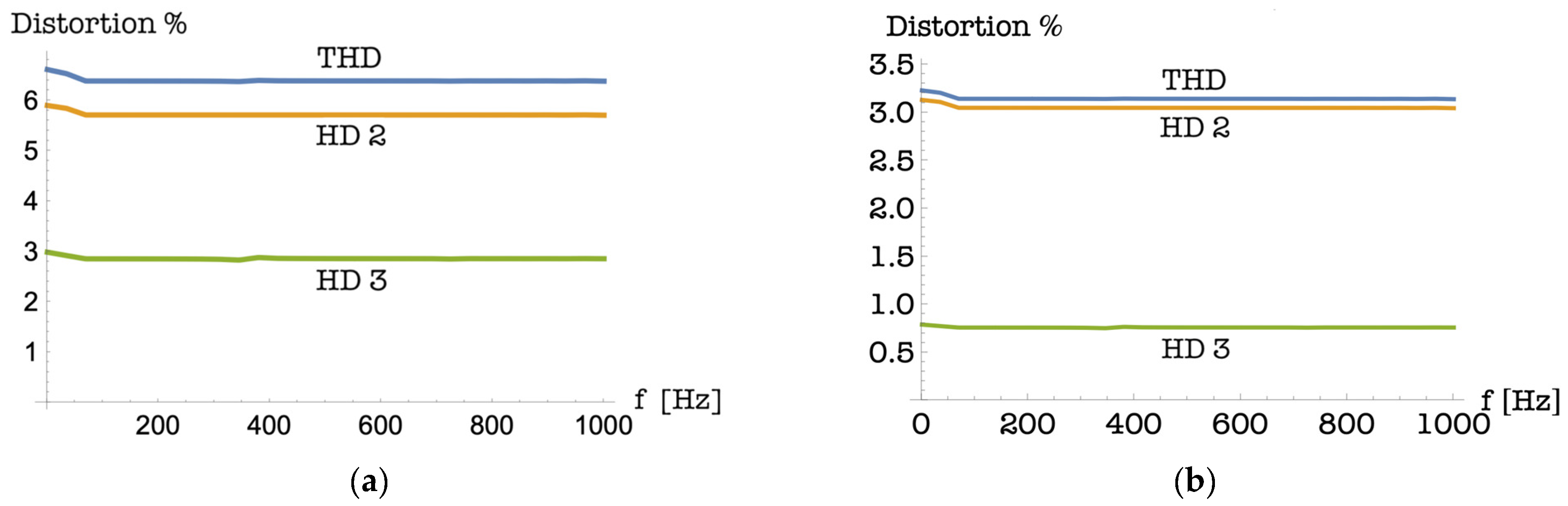
Using the reference parameters (R = 1; Coef = 0.125) we simulated the harmonic distortion estimation procedure that makes use of the PuC technique. We generated an exponential chirp signal characterized by fMin = 10 [Hz]; fMax = 1000 [Hz]; T = 0.47 [s] which was input to the nonlinear system. The output generated by the nonlinear system was used to feed the filter matched to the chirp signal input. From the output of the matched filter, we took the different impulse functions of the vector $\left[g\left(t\right)\right]$. Combining the transforms of these functions according to (16), we obtained the trends of Figure 2a as estimates of $THD$, $H{D}_2$ and $H{D}_3$.

It is evident from Figure 2 that there is an almost constant frequency trend of the estimated value, apart from the very low frequencies, and that these values estimated through the PuC technique are very good estimates of the analytical reference values. Panel (b) of the same figure allows us to verify the quality of the estimate obtained by extrapolation using the technique proposed in this paper: we started from the parameters of the Hammerstein model identified with an input signal of amplitude R = 1, and using the technique proposed in this paper—and in particular formula (12)—we obtained by extrapolation the parameters of the model associated with the amplitude of the excitation signal R = 0.5. Using these extrapolated parameters, we estimated the distortion trends that are reported in panel (b) of Figure 2. Also, the values obtained by extrapolation from a measurement made with a different amplitude of the input signal, are shown to be very good estimates of the distortion parameters, the values of which are given in formula (21).

In Section 2.3, we have shown that it is possible to obtain estimates of the $g_{IMD}\left(t\right)$ functions associated with intermodulation components starting from the $h\left(t\right)$ kernels that identify the Hammerstein model of the nonlinear system. We estimated the $g_{THD}\left(t\right)$ functions that were needed to estimate $THD$, $H{D}_2$ and $H{D}_3$. From these, we estimated the kernels $h\left(t\right)$ and thus the functions $g_{IMD}\left(t\right)$ associated with the intermodulation components. We preliminarily calculated analytically, for both harmonic and intermodulation distortions, the reference values with which to compare the results of the PuC estimation.

Let us then consider the superposition of two sinusoidal signals of equal amplitude: $x\left(t\right)=R \left\{Cos\left[{\omega }_{1}t\right]+Cos\left[{\omega }_{2}t\right]\right\}$ develop and recombine among themselves the powers of the signal placed at the input; thus, it is possible to calculate the values of intermodulation distortions of various types, such as the intermodulation distortion related to the frequency component $f_2-f_1$. Considering the same parameter values used previously (R = 1; Coef = 0.125), we obtained from the analytical calculation of intermodulation distortion the value $IM{D}_{f_2-f_1}=4.87\%$.

To compare this value with that obtained from the PuC procedures proposed in this paper, we started from the impulsive functions $g_{THD}\left(t\right)$ used for estimating the harmonic distortion; through (8) we obtain the trends of the kernels $h\left(t\right)$ that identify the Hammerstein model of the nonlinear system. From these trends, we obtained an estimate of the impulsive functions associated with intermodulation distortion: in particular, we used expression (13) to estimate the first elements of the vector of functions associated, this time, with the intermodulation harmonic components.

In our experiment we used $g_{f_2-f_1}\left(t\right)$, the second trend of the intermodulation vector $g\left(t\right)$ in (13), to estimate that intermodulation component. We were thus able to compare the result of the estimation obtained by starting from a single sine wave excitation, and then move on to the estimation of the parameters $g\left(t\right)$ related to harmonic distortion; from these you have kernels identifying the Hammerstein model, and from these, through the $\left[A_{\mathrm{IMD}}\right]$ matrix, the intermodulation distortion related to the frequency component $f_2-f_1$, with the result calculated analytically.

The result is as shown in Figure 3: It is evident that, despite the complexity of the procedure, the estimated value approximates what had been calculated analytically. Moreover, it is also evident in this case that the fact that the nonlinear system is memoryless results in constant frequency trends of the quantities estimated through the PuC technique.

The verifications described so far have the undoubted advantage of allowing a comparison of analytically calculated parameter values, which thus constitute definite references, with parameters estimated using the proposed procedures based on the PuC technique. The limitation of the tests described lies in the fact that, since it is a nonlinear system without memory, the trends as a function of the estimated quantities have constant trends in frequency, not depending on that variable. To show the effectiveness of the described procedures also in the case of systems with memory, we report the trends estimated with the PuC techniques in the case of two experiments related to nondestructive diagnostics techniques, in one case associated with the verification of a system of metal type, in the other with the verification of a system consisting of concrete beams of the type used in civil construction.

3.2. Damaged Metallic Structure

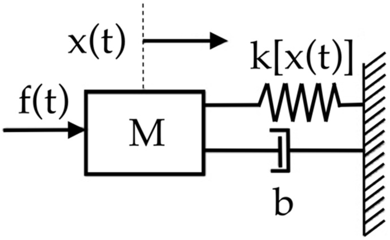
Simulation experiments of a damaged metallic structure were carried out to verify the effectiveness of the proposed method. The damage index HI, proposed in [15], is defined by (19). The model used for the structure is the one already proposed in [16] and used in the experiments in [15]: the system is a one degree of freedom spring-mass-damper (SMD) of the type shown in Figure 4. The damage that has been considered is represented by a bi-linear stiffness k[x(t)], which allows for the simulation of a breathing fracture [16]: a lower stiffness when the fracture is open than when it is closed.

The bi-linear stiffness has been defined as follows:

$$k\left[x\left(t\right)\right]=\left\{\begin{array}{c}{\mathrm{k}}^I\\ \left(1-\alpha \right){\mathrm{k}}^I\end{array}\right..$$

(22)

where ${\mathrm{k}}^I$ is the stiffness of the undamaged system and $\alpha$ is the parameter representing the extent of damage if $\alpha =0$ the system is intact. If $\alpha =1$, the fracture is open and the system is completely damaged.

We generated data from the system defined in Figure 4 and by relation (22) using the following parameters: M = 1 [kg], b = 2 [N s/m] and ${\mathrm{k}}^I=20,000$ [N/m].

Taking into account that the resonance frequency of the simulated system is 22.5 [Hz], an exponential chirp signal operating in the frequency range between 2.25 and 225 [Hz] was used as an input for the identification of the Hammerstein model. The excitation duration was T = 9.36 [s]. For an input amplitude E = 0.1 [N] the output signal maximum absolute value $\left|x_{MAX}\right|$ is of the order of $4\ast {10}^{-5}$ [m].

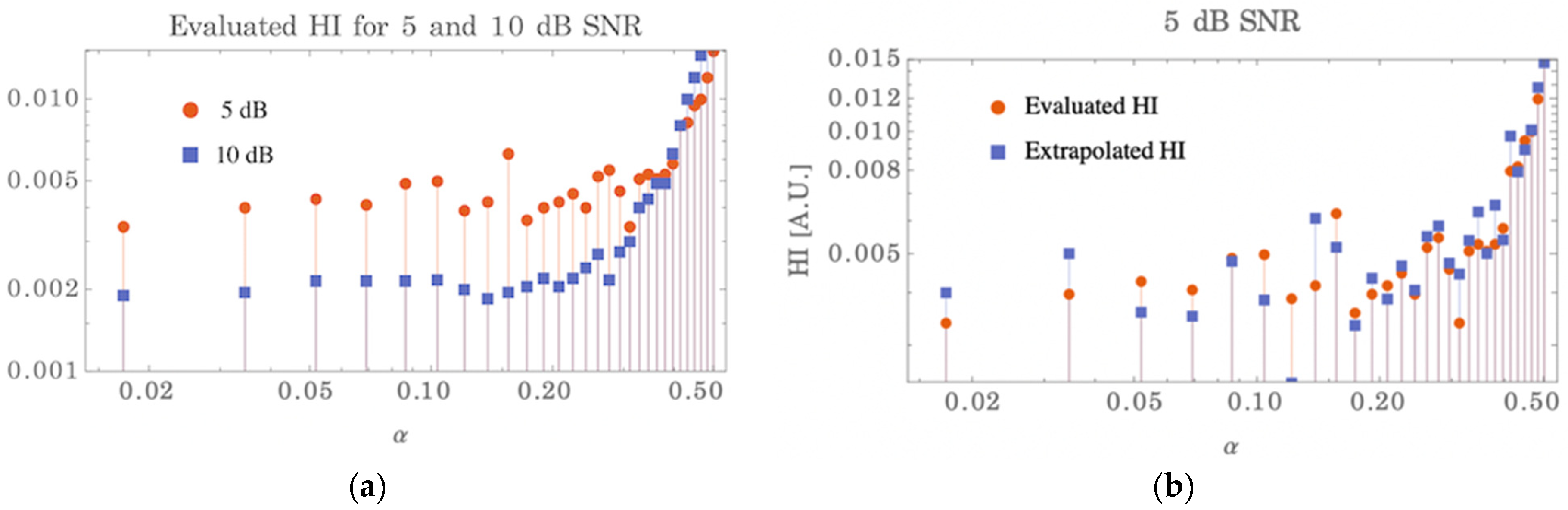
To verify the effectiveness of the methodologies proposed in this paper, the damage index HI was estimated, in a range of values of parameter $\alpha$ between 0.01 and 0.50, for two different signal levels, chosen in order to guarantee signal-to-noise ratios of 10 and 5 dB, respectively: the estimate for the signal-to-noise ratio of 5 dB was also obtained by extrapolating the Hammerstein model parameters obtained in the 10 dB case through expression (12). Figure 5 shows the results obtained for the HI index as the parameter $\alpha$ varies: the left panel in the case where the amplitude of the excitation signal guarantees a signal-to-noise ratio of 10 dB. The right panel shows two curves, both related to a signal-to-noise ratio of 5 dB. Of the two curves, one is obtained by decreasing the amplitude of the excitation signal adopted; the other was obtained by extrapolating the parameters of the Hammerstein model from the 10 dB case, using (12). It is evident from the right panel how the trends of the two curves provide equivalent information and show a knee of the curve near the same $\alpha \cong 0.20$ value. Thus, (12) allows to obtain with good approximation the trends of the HI index as $\alpha$ varies at signal levels other than the one actually used.

3.3. Laboratory Measures on Damaged Concrete Structures

The validity of the technique was also verified in connection with an experiment to test for cracks in a concrete structure: the experiment was performed on a prism-shaped concrete specimen measuring 4 × 4 × 16 cm³; a U-shaped notch with a cross-section of 4 × 4 mm² was made halfway along the length of a 16 cm face of the specimen. The concrete matrix was produced using a CEMI 52.5 R cement, a water-to-cement ratio of 0.5 and a cement-to-sand ratio of 1:3 by weight. The specimen was damaged by subjecting it to a three-point bending loading procedure with controlled displacement rate at the edge of the notch. This procedure created a small crack at the end of the cycle whose size is of the order of 40% compared to the cross-section.

Ultrasonic tests were performed on the damaged specimen: using Phenyl Salicylate, two ultrasonic transducers (nominal center frequency at 55 kHz, diameter of 2 cm) were glued to the two ends of the specimen. An arbitrary waveform generator (TiePie handyscope HS5) was used to produce an exponential chirp signal in the frequency band from 40 to 60 kHz with a duration of about 0.4 s, sampled at 2.5 MHz. The amplitude of the source signals was increased from 10 mV to 1.5 V (before amplification). The signal was then amplified by a factor of 20 before feeding it to the Tx transducer (Falco-System power amplifier). The Rx transducer was connected to an oscilloscope for data acquisition (TiePie handyscope HS5 used as oscilloscope data logger). Figure 6 shows a schematic representation of the stressed bar and the measuring bench.

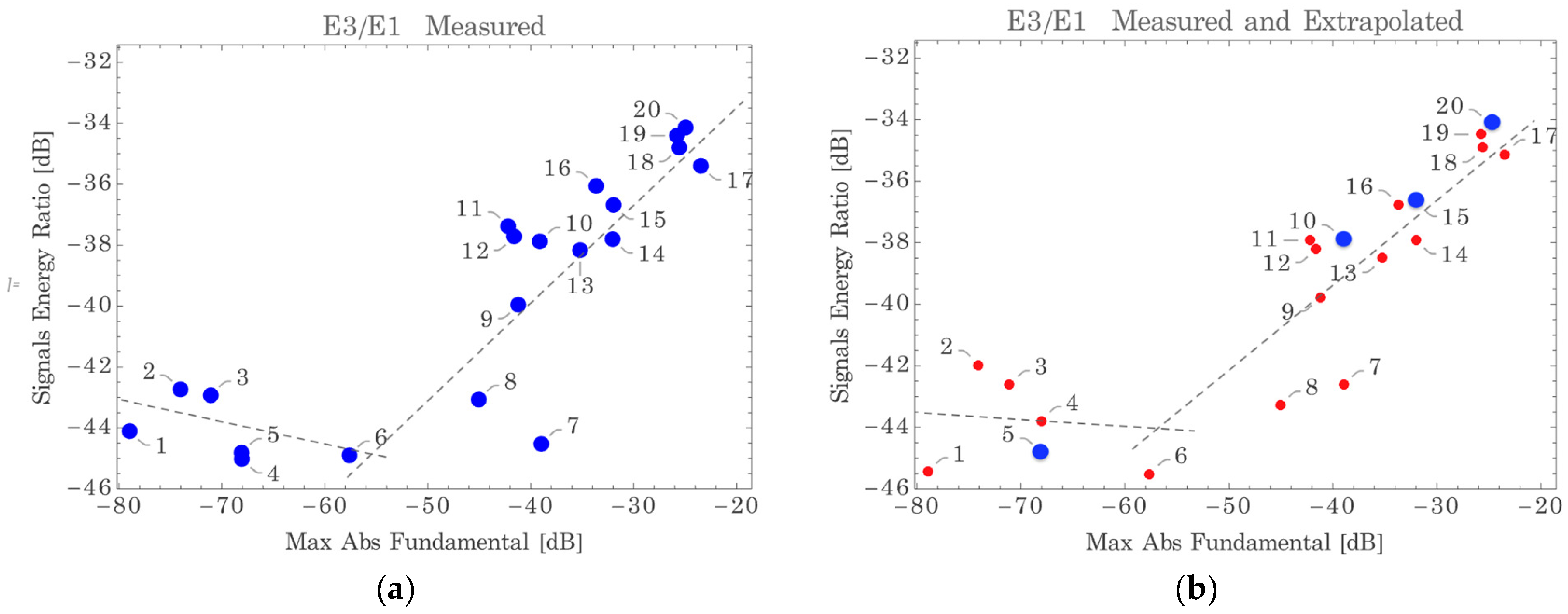
For each of the input signal amplitudes, the Hammerstein model was estimated from the received signal by means of the PuC technique. For each amplitude, the ratio between energy of the signals associated with the third harmonic and with the fundamental was then calculated: a change in the slope of the curve as the amplitude of the excitation signal increases highlights the onset of nonlinear behavior, and thus the presence of a microcrack.

The results of the comparison are shown in the two panels in Figure 7: the left panel shows the $E_3/E_1$ ratio for 20 different input signal amplitudes. The right panel shows the trend of the same ratio having considered the measurement results for only four amplitudes, the points of which are highlighted in the figure, and having extrapolated from this, via (12), the value of the ratio for the other amplitudes. The values reported with red points were estimated starting from the measured points 5, 10, 15 and 20. From each of these values the extrapolation for the four lower levels of input signal was evaluated. In both panels the dotted lines represent linear interpolations on the first group of points (from 1 to 5) and on the remaining 15 points. The abscissa of both panels is the amplitude of the signal received, measured as the maximum of the absolute value of the fundamental in the response to the excitation signal.

Comparison of the two graphs shows substantial equivalence between the two trends, with the knee of the curve at the same amplitude range. Thus, the validity of the extrapolation technique proposed in this paper remains confirmed here as well.

4. Discussion and Conclusions

Having tools to highlight the presence of nonlinearity in a system, and analyze its nonlinearity characteristics, allows us to evaluate the quality of the system itself or the presence of anomalies or defects in the system structure, in many applications. These aspects are often highlighted by global indicators: examples in this sense are the measures of the distortion introduced by a system (electronics, telecommunications [17,18]), or some damage indexes used to evaluate the presence or onset of anomalies in structures subjected to strong stresses (buildings, bridges, and viaducts [19,20,21]). These global indicators can be evaluated by analyzing the system response to known type of stresses, according to the requirements of the various regulations.

The development of increasingly efficient and sophisticated techniques for the modeling representation of the nonlinear system allows us to define a different approach for the evaluation of the same indicators. For example, it has been demonstrated that, within the limits of validity of Hammerstein models, an effective representation of the nonlinear system can be obtained, and from the parameters of the system representation, reliable estimates of the global indicators can be obtained [14,15].

The system represented obviously must have the characteristics that allow its representation through a Volterra model, or a model derived from it, such as the Hammerstein model. The approximate nonlinear system must be characterized by “fading memory”; that is, the system response must depend less and less on past inputs as we move away in time. It follows that this constraint excludes systems whose output depends substantially on the initial conditions and on input values far in the past, such as those characterized by chaotic behaviors. Furthermore, as far as input signals are concerned, representability through Volterra series requires that the inputs are sufficiently “smooth” and do not show variations that are too abrupt, which excludes, for example, piecewise constant input signals [22]. A very wide variety of systems of engineering interest can therefore be validly represented in terms of their nonlinear characteristics by models such as the Hammerstein model, adopted in the present work, whose identification can be effectively obtained through the PuC technique, as is widely verified in the technical literature [8,9,10,11,12]. The identification technique we use refers directly to the structure of the Hammerstein model shown in Figure 1: variants to this structure have been proposed in an attempt to use a modeling technique derived from Hammerstein’s also to nonlinear systems of chaotic type [23,24]. The technique proposed in this paper, valid in most applications, is not applicable to the special case of modeling nonlinear systems of chaotic type.

In the present work we have proposed two original contributions related to the estimation of global parameters starting from the Hammerstein model: the first is related to the possibility, through a variant of the PuC technique for the identification of the Hammerstein model, of obtaining estimates of global parameters, as the distortion or damage indexes, relating to signal levels different from the one actually used for the experiments. This possibility allows us to reduce the number of laboratory experiments necessary to obtain a picture of the effects on the nonlinearity of the signal input levels. In particular, in Section 2.2, we have shown that from the pattern identified by an excitation signal of a specific amplitude, it is possible to obtain the patterns that would have been obtained from different amplitudes of the excitation signal, thus allowing us to obtain a full range of synthetic parameters (distortion, damage index) from making a single measurement.

The second original contribution is a procedure that shows how the PuC technique can be used in the case of more than one type of input signal and is not limited to the single exponential swept sine signal. Whatever the input signal, if we are able to obtain the Hammerstein model from it, then it is from this model that we can obtain the global parameters that would have required input signals different from the one actually used. In Section 2.3, we have shown that the identification technique based on pulse compression can be used not only by using an exponential swept sine signal, but also by using a signal of a different type, provided that for the signal chosen as input, the corresponding transformation matrix is defined, which binds the powers of the chosen signal to its respective harmonics.

Also, in this case the practical advantage can be considerable in terms of reduction in the laboratory tests necessary to obtain a vast range of indicators; if, from a single set of measurements, we obtain a valid model of the nonlinear system, from this model we can also obtain the other indicators, which would have required experiments with input signals of different types.

We have sought applications in very different fields to accurately verify the validity of the two original proposals put forward in this work: the experiments are related to distortion estimates, a topic specific to telecommunications and electronics; two experiments are specific to nondestructive diagnostics, one is related to a simulation of damage in metallic materials, and the second is related to the verification of the presence of damage in civil concrete structures. This second application is directly linked to the project “Integration of Artificial Intelligence and Ultrasonic Techniques for Monitoring Control and Self-Repair of Civil Concrete Structures (CAIUS)” which financially supports the present research activity, and it is on this application that the research group is currently developing the proposed techniques. Regarding the future developments of this research activity, we are currently further developing the activity by extensively applying the developed techniques to cementitious materials through the implementation of several additional laboratory measurements. We are also working to carry out an analysis of the error and sensitivity of the extrapolation methods of different estimators as a function of the parameters measured during data acquisition.