A Method to Obtain the Transducers Impulse Response (TIR) in Photoacoustic Imaging

Abstract

Photoacoustic tomography (PAT) is an emerging imaging technique with great potential for a wide range of biomedical imaging applications. The transducers impulse response (TIR) is a key factor affecting the performance of photoacoustic imaging (PAI). It is customary in PAI to assume that TIR is known or obtain it from experiments. In this paper, we investigate the possibility of obtaining TIR in another way. A new method is proposed to extract TIR from observed optoacoustic signal (OPAS) data, without prior knowledge, as a known condition. It is based on the relation between the OPAS data and the photoacoustic pressure signal (PAPS) at transducer positions. The relation can be expressed as a homogeneous linear equation. The TIR is solved by solving the homogeneous equation. The numerical test verifies the effectiveness of the presented method. This article also discusses the effect of calculation parameters on the extracting precision of TIR.

1. Introduction

As a new imaging method for biological tissues, photoacoustic imaging (PAI) combines the advantages of high contrast in optical imaging and high resolution in ultrasonic imaging. It uses a short-pulse laser as an excitation source to irradiate biological tissue. The optical absorption area inside the sample will undergo isobaric expansion and radiate ultrasonic waves. The acoustic signals resulting from the photoacoustic effect are measured by the use of ultrasonic transducers [1,2]. In recent years, many new advances have been made in ultrasonic transducers, and they have contributed significantly to developments in the field of PAT [3,4,5]. We can reconstruct the spatial distribution of light absorption in a sample using the photoacoustic signals observed by transducers. The spatial distribution of optical absorption inside the sample can be reconstructed from the observed photoacoustic signal (OPAS). PAI provides structural and functional imaging in different application areas, such as vascular imaging [6,7,8], brain imaging [9,10,11,12], breast cancer imaging [13,14,15,16,17], and sentinel lymph node imaging [18,19,20,21].

The resolution of PAI (PAI resolution refers to the sharpness of the image and the amount of information stored in the image) depends on not only the performance of the reconstruction algorithm but also the quality of OPAS. Many reconstruction algorithms usually assume the observation condition is ideal and that the OPAS is the real photoacoustic pressure signal (PAPS) at the transducer positions. However, some factors affect OPAS. Among them, the bandwidth of the transducer is an important one. The TIR of limited bandwidth transducers will deform the waveform of OPAS, and then cause blur in the reconstruction image. TIR is affected not only by the temporal impulse response, but also by the spatial impulse response [22,23]. To eliminate this effect, Geng Ku applied temporal data deconvolution methods to filter the back-projection algorithm for photoacoustic tomography (PAT) [24]. Yae-linSheu used the filtered back-projection algorithm for intravascular PAI [25]. TIR was incorporated into the system matrix to reduce the aroused distortion in the intravascular reconstruction. These studies were conducted under the premise that TIR was known. However, when TIR is unknown, Chen Yang proposed a method combining hybrid weighted adaptive total variation to improve the image quality of PAT [26]. Nikita Rathi proposed the estimation of the impulse response of photoacoustic systems using homomorphic filtering based on discrete wavelet transform [27]. The proposed method was implemented on experimentally collected photoacoustic data generated from different phantoms and verified through simulation studies with the same photoacoustic targets as the experimental study phantoms.

Knowing TIR is the key to eliminating its effect on OPAS. So far, it is usually obtained by experiment measuring. Kruger et al., Xu, and Wang propose a method to measure TIR by irradiating the transducer with a weak laser pulse [28,29]. Yi Wang proposed a deconvolution-based PAI reconstruction method [30]. This method deconvolves the OPAS from the point light source with the OPAS from the sample. A projection of the light absorption distribution of the sample can be obtained directly. Tao Lu proposed a method to generate TIR using point-absorbing materials [31]. Li Qi proposed a PAT image restoration method based on experimentally measured spatially varying TIR to improve image quality and resolution [32]. All the above obtain TIR through experiments. Such measurements not only increase the complexity of the experiment but also make it difficult to ensure experimental accuracy.

This paper examines another method for obtaining a TIR for a limited bandwidth transducer. This is a method that does not require any prior knowledge as a known condition to extract TIR directly from OPAS. It is based on the relationship between OPAS and PAPS data at different observation locations. This relationship can be expressed as a system of homogeneous linear equations, and the PAPS results are obtained by solving homogeneous linear equations. Numerical experiments verify the effectiveness of the proposed method. And the influence of calculation parameters on the accuracy of TIR extraction is also discussed.

2. Basic Principles of Solving TIR

Light absorbance results in transient local heating and a pressure increase in proportion to the absorbed light energy. This leads to the creation of pressure waves. The propagation of photoacoustic pressure waves may be given through a generic wave equation [30].

$$({\nabla }^2-\frac{1}{v^2}\frac{{\partial }^2}{\partial t^2})x(\mathbf{r},t)=-\frac{\beta }{C_p}\frac{\partial }{\partial t}\delta (\mathbf{r},t),$$

(1)

where r denotes the coordinates of any position in 3D space, t is time, v is the speed of sound, β is the coefficient for expansion of isobaric volume, and C_p is constant pressure-specific heat. $\delta$ is the heat source function. We know that TIR is affected not only by the temporal impulse response, but also by the spatial impulse response [22,23]. Because the transducer used in the simulation in this paper is a point-like transducer [33,34,35], its size is close to a point and can be ignored. Moreover, the simulation in this paper is based on far-field detection, which means that the distance between the support and the transducer is much longer than the wavelength corresponding to the center frequency of the detection device. In this article, we only consider temporal TIR. The PAPS at time t can be expressed as

$$x(t)=\frac{\beta }{4\pi C_p}{\displaystyle \iiint \frac{d\mathbf{r}}{\mathbf{r}}}\frac{\partial \delta (\mathbf{r},t\text{'})}{\partial t\text{'}}{|}_{t\text{'}=t-\frac{\mathbf{r}}{v}},$$

(2)

where r = |r|. If the transducer is limited by the bandwidth, then the OPAS is affected by the TIR and the obtained OPAS signal at the transducer becomes [36]

$$y(t)=h(t)\ast x(t),$$

(3)

where y(t) is the OPAS, x(t) is the PAPS, and h(t) is the TIR in this PAI system.

To simplify the convolution operation in the time domain, it is transformed to the frequency domain through Fourier transform. So, when the number of transducers is 𝐽 and by assuming that all the transducers have the same TIR (in this article, the transducers we use are made by the same manufacturer and the same model; all TIRs are considered to be the same), the following equation can be obtained

$$H(\omega )=\frac{Y_1(\omega )}{X_1(\omega )}=\frac{Y_2(\omega )}{X_2(\omega )}=\cdots =\frac{Y_J(\omega )}{X_J(\omega )}.$$

(4)

Here, 𝐻(𝜔), 𝑌_𝑗(𝜔), and 𝑋_𝑗(𝜔) are the TIR, the OPAS, and the PAPS after the Fourier transform, respectively, 𝑗 = 1, 2, …, 𝐽. Suppose there are only two transducers and j = 1, 2; then, the equation is

$$Y_2(\omega )X_1(\omega )-Y_1(\omega )X_2(\omega )=0.$$

(5)

Perform the inverse Fourier transform of Equation (5) to obtain the equation for the time domain:

$$y_2(t)\ast x_1(t)-y_1(t)\ast x_2(t)=0.$$

(6)

Discretize the continuous function of the time domain:

$$y_2(k)\ast x_1(k)-y_1(k)\ast x_2(k)=0.$$

(7)

Then, write the above equation in matrix form:

$${\mathit{Y}}_2{\mathbf{x}}_1-{\mathit{Y}}_1{\mathbf{x}}_2=0,$$

(8)

where matrices Y₁ and Y₂ are the called convolutional matrices, or simply C–matrices.

$${\mathit{Y}}_j(0)=\left(\begin{array}{ccccc}{a}_{1,j}& 0& \dots & 0& 0\\ a_{2,j}& a_{1,j}& \dots & 0& 0\\ ⋮& ⋮& \ddots & ⋮& ⋮\\ 0& 0& \cdots & a_{M,j}& a_{M-1,j}\\ 0& 0& \cdots & 0& a_{M,j}\end{array}\right)$$

(9)

where 𝑎_𝑗 is the OPAS data from the 𝑗-th sensor. The first column of the matrix consists of M data of the OPAS, appended K − 1 zeros, M is the size of the OPAS vector, and K is the size of the PAPS vector. The other columns are cyclic copies of the first column. Similarly, L is the size of the TIR vector h. The relationship between them is

$$M=K+L-1.$$

(10)

Generalization to two or more transducers:

$$M_j=K_j+L-1.$$

(11)

Then, Equation (8) can be written as a homogeneous linear system:

$$\widehat{\mathit{Y}}\widehat{\mathbf{x}}=0.$$

(12)

where $\widehat{\mathit{Y}}$ consists of two matrices, Y₂ and −Y_1:

$$\widehat{\mathit{Y}}=({\mathit{Y}}_2-{\mathit{Y}}_1),$$

(13)

where the number of columns Y₁ is equivalent to K₂, that is, the size of the vector x₂; similarly, the number of columns Y₂ is equivalent to K₁, which is the size of the vector x₁. So, the matrix is assured as a block matrix of (K₁ + M₂ − 1) multiplied by (K₁ + K₂). And the vector $\widehat{x}$ is

$$\widehat{\mathbf{x}}=\left(\begin{array}{c}{\mathbf{x}}_1\\ {\mathbf{x}}_2\end{array}\right).$$

(14)

The above equation can be generalized to more than two transducers. For J > 2, the equation can be formed as

$$Y_j(\omega )X_k(\omega )-Y_k(\omega )X_j(\omega )=0,$$

(15)

and

$$j=k(\mathrm{mod}J)+1.(j\ne k).$$

(16)

Then, we can obtain J(J − 1)/2 equations. Similarly, Equation (12) can be acquired, and

$$\widehat{\mathit{Y}}=\left(\begin{array}{cccccc}{\mathit{Y}}_2& -{\mathit{Y}}_1& & & & \\ {\mathit{Y}}_3& & -{\mathit{Y}}_1& & & \\ {\mathit{Y}}_4& & & -{\mathit{Y}}_1& & \\ ⋮& & & & \ddots & \\ & {\mathit{Y}}_3& -{\mathit{Y}}_2& & & \\ & {\mathit{Y}}_4& & -{\mathit{Y}}_2& & \\ & ⋮& & & \ddots & \\ & & & {\mathit{Y}}_{J-1}& -{\mathit{Y}}_{J-2}& \\ & & & {\mathit{Y}}_J& & -{\mathit{Y}}_{J-2}\\ & & & & {\mathit{Y}}_J& -{\mathit{Y}}_{J-1}\end{array}\right).$$

(17)

Y_j is C-matrices (the blank part of Equation (17) is 0). Here, Equation (17) is the sparse block matrix. Solving Equation (18) can obtain the PAPS. And vector $\widehat{x}$ is

$$\widehat{\mathbf{x}}=\left(\begin{array}{c}{\mathbf{x}}_1\\ {\mathbf{x}}_2\\ ⋮\\ {\mathbf{x}}_J\end{array}\right).$$

(18)

After the PAPS is obtained, the TIR can be obtained according to the relationship between the PAPS and the OPAS.

3. Algorithms

For solving the photoacoustic pressure vector x in Equation (12), it is multiplied by the transpose matrix of $\widehat{\mathit{Y}}\left(\mathit{K}\right)$, and we obtain [36]

$${\widehat{\mathit{Y}}}^T\widehat{\mathit{Y}}\widehat{\mathbf{x}}=0.$$

(19)

We define it as the matrix $\widehat{\mathit{E}}={\widehat{\mathit{Y}}}^T\widehat{\mathit{Y}}$, which is a square matrix. The PAPS vector $\widehat{x}$ is the solution of Equation (19). It must be the eigenvector with zero-eigenvalue of the matrix $\widehat{\mathit{E}}$. If the matrix $\widehat{\mathit{E}}$ has only one zero-eigenvalue, then the eigenvector corresponding to this zero-eigenvalue is the PAPS vector.

The matrix $\widehat{\mathit{Y}}$ consists of some C-matrices, and each C-matrix consists of a cyclic arrangement of PAPS vectors, the same as Equation (9). This vector is the convolution result of the PAPS vector and the TIR vector. Such characteristic matrix $\widehat{\mathit{Y}}$ make the matrix $\widehat{\mathit{E}}$ have special properties. The matrix $\widehat{\mathit{E}}$ has only one zero-eigenvalue. By working out the eigenvector corresponding to this zero-eigenvalue of the matrix $\widehat{\mathit{E}}$, the PAPS vector can be obtained.

The above mathematical derivation and results assume that the length of the OPAS data is equal to the sum of TIR and the PAPS lengths, and they are all known. However, this assumption cannot be guaranteed in actual computation. The size of the PAPS is usually equal to that of the OPAS, or the lengths of the PAPS and TIR data are not known. In this situation, are the above derivation and results valid?

In actual measurements, the OPAS is generated by finite biological tissues; therefore, the length of the OPAS is finite. We can obtain the whole of the OPAS as long as the record length is enough. In this case, the tail of the OPAS is characterized by gradual attenuation, so the deviation of reality from the assumption that the length of the OPAS is equal to the sum of TIR and PAPS lengths is little. In other words, the data in the part where the tail goes to zero can be assumed to have little effect on the results.

The structure of the matrix $\widehat{\mathit{Y}}$ is dependent on not only the OPAS data but also the length of PAPS. It is needed to know the length of the PAPS before solving Equation (19) to define the matrix $\widehat{\mathit{E}}$. It is hard to know the length of the PAPS according to actual photoacoustic signal observation, but we can fix it based on the property of the matrix $\widehat{\mathit{E}}$. When the deviation from the actual size of the PAPS occurs, the number of zero-eigenvalue of the matrix $\widehat{\mathit{E}}$ will change. The number of zero-eigenvalue of the matrix $\widehat{\mathit{E}}$ is equal to the deviation from the actual size of the PAPS. We therefore can determine the size of the PAPS vector in the light of the number of zero-eigenvalue of the matrix $\widehat{\mathit{E}}$.

Based on the above analysis, The following steps are used to obtain the PAPS vector.

(1) Firstly, assuming K = M, calculate the $m$ minimum eigenvalues of $\widehat{\mathit{E}}\left(M\right)$. Where m = min (M_j) (since the signal length of the PAPS cannot be longer than the shortest OPAS length, i.e., K ≤ m, this involves all potentialities); and identify the number of the zero-eigenvalues of $\widehat{\mathit{E}}\left(K\right)$. In the case of only one zero-eigenvalue, the value of the PAPS length K can be found.

For simplicity, the singular value decomposition (SVD) of the matrix $\widehat{\mathit{Y}}$ can be calculated to determine the zero-eigenvalues of the matrix $\widehat{\mathit{E}}\left(M\right)$.

$$\widehat{\mathit{Y}}=\mathit{U}\mathit{S}{\mathit{V}}^T.$$

(20)

The column of the matrix V is the right singular vector of $\widehat{\mathit{Y}}$ and is the eigenvector of $\widehat{\mathit{E}}={\widehat{\mathit{Y}}}^T\widehat{\mathit{Y}}$. S is a diagonal matrix. The element along the diagonal of S is called the singular value of $\widehat{\mathit{Y}}$ and is equal to the positive square root of the eigenvalues of ${\widehat{\mathit{Y}}}^T\widehat{\mathit{Y}}$.

In this step, only the number of singular values which are equal to zero needs to be required. In the next step, the singular vector corresponding to the smallest singular value is used. It is the array of the PAPS.

(2) Recalculate the eigenvector that $\widehat{\mathit{E}}\left(K\right)$ has only one minimum eigenvalue (the numerical infinitely approaches zero). This eigenvector is the array of the PAPS. Break down the eigenvectors into J-group PAPS, and the length of the PAPS obtained for each transducer is K.

(3) TIR is found by the LS algorithm. It maps each of these J PAPS arrays to the corresponding transducer.

When the matrix is solved, the result is only one of the general solutions, which may lead to the opposite result of the experiment. In this case, the PAPS needs to be determined to be correct. As in experiments and simulations, the starting point of the power amplifier signal always tends to rise. If the result is contrary to this, then it needs to be corrected by adding a minus sign in front of the PAPS data and then continuing to solve for the TIR.

Next, the LS algorithm for solving the TIR in step (3) is introduced. In some optimization problems, such as curve-fitting problems, the objective function consists of the sum of squares of several functions [37,38]. It can generally be written as

$$F(\mathbf{h})={\displaystyle \sum _{i=1}^M{f}_i^2(\mathbf{h})},$$

(21)

in (21), we assume

$$f_i(\mathbf{h})=x_i\ast \mathbf{h}-{\mathbf{y}}_i.i=1,2,\cdots ,M,$$

(22)

where $\mathbf{h}={({\mathbf{h}}_1,{\mathbf{h}}_2,\dots ,{\mathbf{h}}_L)}^T$, which is the TIR vector of the transducer. The general assumption is that M ≥ L. Where x_i is the PAPS vector and y_i is the OPAS vector, Equation (22) is expressed in matrix form as

$$f_i(\mathbf{h})=\mathbf{A}\mathbf{h}-\mathbf{B}=0,$$

(23)

where A is the C-matrix composed of the PAPS, and it is a matrix of M by L-dimensional. B is a matrix of OPAS, which is an M-dimensional column vector.

Let A be full rank, and A^TA is a symmetric positive-definite matrix of order n. The TIR formula derived from the LS algorithm derived from the literature [38] is

$$\mathbf{h}={({\mathbf{A}}^T\mathbf{A})}^{-1}{\mathbf{A}}^T\mathbf{B}.$$

(24)

For linear LS problems, as long as A^TA is not singular, it can be solved with the Formula (24). Then, the resulting h is the TIR signal.

It should be noted that the algorithm in this paper is not suitable for regular-shaped circular and spherical biological tissue models. Under normal circumstances, we will arrange all transducers in a ring. If the shape of the measured biological tissue is round or spherical, and it is placed in the center of the calculation grid, then the OPAS received by each transducer is the same data. Using these data to solve TIR, the linear homogeneous system will be unsolvable. In this case, the method proposed in this paper is not applicable.

If there is noise in OPAS data, then the algorithm must be improved.

The matrix $\widehat{\mathit{E}}$ has two properties:

(1) When the correct value of K is determined, the matrix $\widehat{\mathit{E}}$ has only one zero-eigenvalue and its corresponding eigenvector is PAPS.

(2) If the value of K cannot be determined, the matrix $\widehat{\mathit{E}}$ has more than one zero-eigenvalue. If we determine that K = K’ (K’ is not the correct length of the PAPS signal), then the matrix $\widehat{\mathit{E}}$ will find L = K’ − K + 1 zero-eigenvalues. Accordingly, these zero eigenvectors will have the following structure:

$$\mathbf{r}=\left(\begin{array}{c}{\mathbf{r}}_1\\ 0\\ ⋮\\ 0\\ {\mathbf{r}}_2\\ 0\\ ⋮\\ {\mathbf{r}}_J\end{array}\right).$$

(25)

If the length of the OPAS received by each transducer is M, then r will be a (MJ – L + 1)-dimensional vector, J is the number of transducers, consisting of components r₁ to r_j, and each vector (except the first, of course) has L − 1 zeros between it and the previous one.

$${\mathbf{v}}_j=\mathbf{r}\ast {\mathbf{u}}_j=\mathit{R}{\mathbf{u}}_j={\mathit{U}}_j\mathbf{r} \mathrm{for} j=1,\dots ,L.$$

(26)

where v_j are L eigenvectors of $\widehat{\mathit{E}}\left(M\right)$ with zero-eigenvalue, r is a (MJ × L)-dimensional C-matrix based on the vector r. We can choose a number J_v representing the number of arrays of eigenvectors v_j and construct a matrix $\widehat{\mathit{V}}$ that is exactly like $\widehat{\mathit{Y}}$, such as Equation (17).

Similarly, $\widehat{\mathit{V}}\left(MJ-L\right)$ has a singular vector, e.g., u whose singular value is zero. It is equal to

$$\mathbf{u}=\left(\begin{array}{c}{\mathbf{u}}_1\\ {\mathbf{u}}_2\\ ⋮\\ {\mathbf{u}}_{Jv}\end{array}\right).$$

(27)

Once we have the vector u_j, we can use (26) to solve for the PAPS.

We will improve the second step of the algorithm.

(2) Next, select the eigenvector corresponding to L minimum eigenvalues. and the minimum eigenvalue of the matrix $\widehat{\mathit{F}}\left(MJ-L\right)={\widehat{\mathit{V}}}^T\left(MJ-L\right)\widehat{\mathit{V}}\left(MJ-L\right)$ and its corresponding eigenvector are calculated. This eigenvector is an array of J groups u. The eigenvectors are decomposed into J_v groups, each of which has a signal length of L. By solving Equation (26), the group J PAPS is calculated.

4. Tests and Discussion

In this part, a k-wave toolbox was used for the simulations of OPAS as well as the reconstruction of the images [39]. The simulation was implemented using MATLAB R2021a on Windows 10 running with 32 GB of memory.

An example verifies whether the algorithm is suitable for research in the field of PAI. This part discusses how to use the algorithm to find the eigenvector corresponding to the minimum eigenvalue, the PAPS. The resulting PAPS is used to obtain the TIR. It also discusses how to select the number of transducers and the signal length of the OPAS to obtain the correct TIR more efficiently and accurately.

4.1. The Ability to Solve the TIR

The digital model of the vascular grid in the K-Wave toolbox will be used to simulate the PAI process and results. Figure 1a describes the photoacoustic data acquisition geometry diagram, and Figure 1b shows the vascular mesh geometry used for the simulation study.

In this paper, the simulation is carried out in 2D (to reduce computational complexity), and the initial pressure of the vascular model is loaded from the image and scale using a computational grid of 128 × 128 pixels. Here, PML (Set PML = 20) is used to satisfy the boundary conditions, the vascular grid is placed in the center of the computational grid, and the number of transducers is 120. Place the transducers clockwise on a 3/4 circle with a radius of 30 mm to simulate the PAI setup. The No. 1 transducer is placed on the far left of the horizontal line in the center of the grid, as shown in Figure 1a. The transducer is assumed to be a point transducer. The simulation assumes a sound velocity of 1500 m/s. The optical absorption coefficient of the vascular model was set to 2 mm⁻¹. For simplicity, the medium is considered acoustically homogeneous and has no absorption or diffusion of sound. Of course, any other medium (acoustically inhomogeneous) can also be considered.

Since the simulated environment is a near-ideal environment, it is assumed to be unaffected by any noise other than TIR. It is necessary to set the TIR to study and verify whether the algorithm is suitable for PAI techniques. Different types of transducers have different TIR, especially in practical applications. However, the ideal TIR model is generally used in the theoretical or simulation research of PAI methods. The center frequency of the transducer was 3 MHz, the photoacoustic data were collected at a sampling rate of 10 MHz, and the number of temporal samples obtained by the sensor was 300. The bandwidth of the transducer set in this article is 80%. Its image in the time domain is shown in Figure 1c. Using MATLAB 2021b for simulation, the hypothetical TIR is convolved with the PAPS to obtain the OPAS.

Here, 120 transducers are used for the calculation, place the transducers clockwise on a 3/4 circle with a radius of 30 mm, and each transducer is 2.25° apart. The signal length of the OPAS data obtained from each transducer in this paper is 339, so the length of PAPS is assumed to be 339 for the calculation of the algorithm, and the size of the smallest 339 eigenvectors taken is compared. Figure 2a is an image of eigenvalues plotted on a logarithmic scale. It can be seen that it drops significantly after the 300th eigenvalue and is significantly smaller compared to other eigenvalues. Then, it can be considered that the eigenvalues from the 300th point to the 339th point are 0. That is, the number of zero-eigenvalues is 40. It can be seen from the algorithm section, that the accurate PAPS can be obtained when there is only one zero-eigenvalue. And then its length is known. Therefore, Figure 2b shows the relative sizes of the smallest 40 eigenvalues when recalculating the eigenvalues in the above case. It can be seen that the last eigenvalue is significantly smaller than the other eigenvalues. The eigenvector associated with this minimum eigenvalue is an array of 120 PAPS. Thus, the array length of the PAPS can be obtained as K = 300. The calculated PAPS of one of the transducers is compared with the original PAPS as shown in Figure 2c. It can be seen that the shape and trend are the same between them, and the calculated results are correct.

The TIR in the PAI system is solved to verify the accuracy of the algorithm. After obtaining the PAPS, the LS algorithm can now be used to solve TIR. Since all transducers used are the same, calculating the TIR selects data from one of the transducers for LS. The PAPS used in the calculation is the data obtained by the algorithm, and its signal length is K = 300. Using (25), the OPAS and PAPS are brought into the equation to obtain the TIR. The TIR image obtained by the LS method (Figure 3) is compared with the hypothetical TIR image (Figure 1b), and it can be seen that the shape of the image and the trend are consistent. Through the above PAI simulation verification, the conclusion that the algorithm can be applied to PAI research based on a deconvolution algorithm is drawn.

4.2. The Effect of the Number of Transducers on the Results

In practical applications, if a large number of transducer data is selected, the calculation time will be greatly increased. Therefore, it is especially important to discuss how to choose the number of transducers. Because two transducers satisfy the condition of finding TIR, verify whether the OPAS data obtained by the two transducers can obtain the correct TIR. We chose 2 transducers, No. 1 and a transducer rotated 90° clockwise from its position around the center of the reconstructed area. As can be seen from Figure 4, when the number of transducers is set to 2, the result of the solved TIR is only a negative sign away from the set TIR.

We calculated the TIR using data of 339 signal lengths from two transducers. As shown in Figure 4, it is found that, sometimes, the TIR solved by the algorithm is different from the set TIR by only one negative sign. At the same time, the resulting PAPS has a negative sign compared to the original PAPS (which is not affected by the TIR). From the point of view of linear algebra, which solves systems of homogeneous linear equations, the result obtained in this case is also correct; the coefficients of the solution are simply different. The result of the convolution of the obtained PAPS and TIR is the same as the OPAS. As shown in Figure 5, in this case, the PAPS obtained by the algorithm can be observed. Meanwhile, the start of the PAPS always tends to be upward in the experiments and simulations. The beginning of the PAPS is obtained by the algorithm in Figure 5 shows a downward trend, which does not correspond to reality.

If this is the case, then the result is in need of correction. When finding the TIR signal, the PAPS first needs to be judged to be true. If this is not carried out, then the PAPS obtained contains one more negative sign than that which actually exists. Next, the PAPS obtained needs to be corrected by adding a negative sign to obtain the result shown in Figure 6a. Then, the LS method is used to solve the problem, and the correct TIR can be obtained, as shown in Figure 6b. Based on this result, data from two of these transducers can be selected to solve the TIR in order to obtain accurate results and shorten the operation time.

4.3. The Effect of OPAS Length of the Transducer on Results

To obtain the TIR more efficiently, it is discussed whether it is possible to obtain an accurate TIR by selecting the length of the OPAS obtained by the transducer. Because the above discussion has concluded that the TIR can be obtained by two transducers, the following discussion defaults to the calculation of the data of the two transducers. The calculation uses data on the length of 339 OPAS from two transducers. We chose two transducers, No. 1 and a transducer rotated 90° clockwise from its position around the center of the reconstructed area. Data of 100 and 200 signal lengths are selected from each of the two transducers’ OPAS. When selecting the signals, they are selected sequentially, starting from the beginning of the OPAS.

Compare the PAPS calculated by the algorithm with the original PAPS. As can be seen in Figure 7, when the OPAS length is 100 (Figure 7a), the calculated PAPS is incorrect. The calculated PAPS when the observed signal length is 200 (Figure 7b) is consistent with the original PAPS. This is because data tending to zero have little effect on the algorithm result, as the OPAS data tends to zero after approximately the 200th signal. The length of TIR was assumed to be 30 or 40 to test whether the correct result could be obtained.

Here, to verify the results, Figure 8 shows the result of calculating the LS algorithm when the OPAS length is 100, assuming that the TIR signal length is 30 or 40. Because the PAPS calculated by the algorithm is wrong, the TIR calculation is also wrong. The reason is that, when selecting OPAS data, it selects biological tissues that produce OPAS that are incomplete, and the selected data no longer satisfy the convolution equation of Equation (1). These data cannot be used to solve the PAPS and TIR.

When continuing to calculate the OPAS length of 200, assuming the TIR length is 30 or 40, the TIR is also calculated with the LS algorithm. As the PAPS was correct earlier, the result of the TIR calculation would also have been correct. The result obtained is shown in Figure 9a,b. It can be seen that the result is not much different from the set TIR. The missing data in Figure 9a are data which are more likely zero, which did not affect the outcome. So, if this article is taken as an example, a signal length of about 200 should be selected for each transducer to obtain an accurate TIR. According to this conclusion, in practice, when solving the TIR by selecting the OPAS length, intact OPAS produced by biological tissues should be selected to obtain the correct TIR.

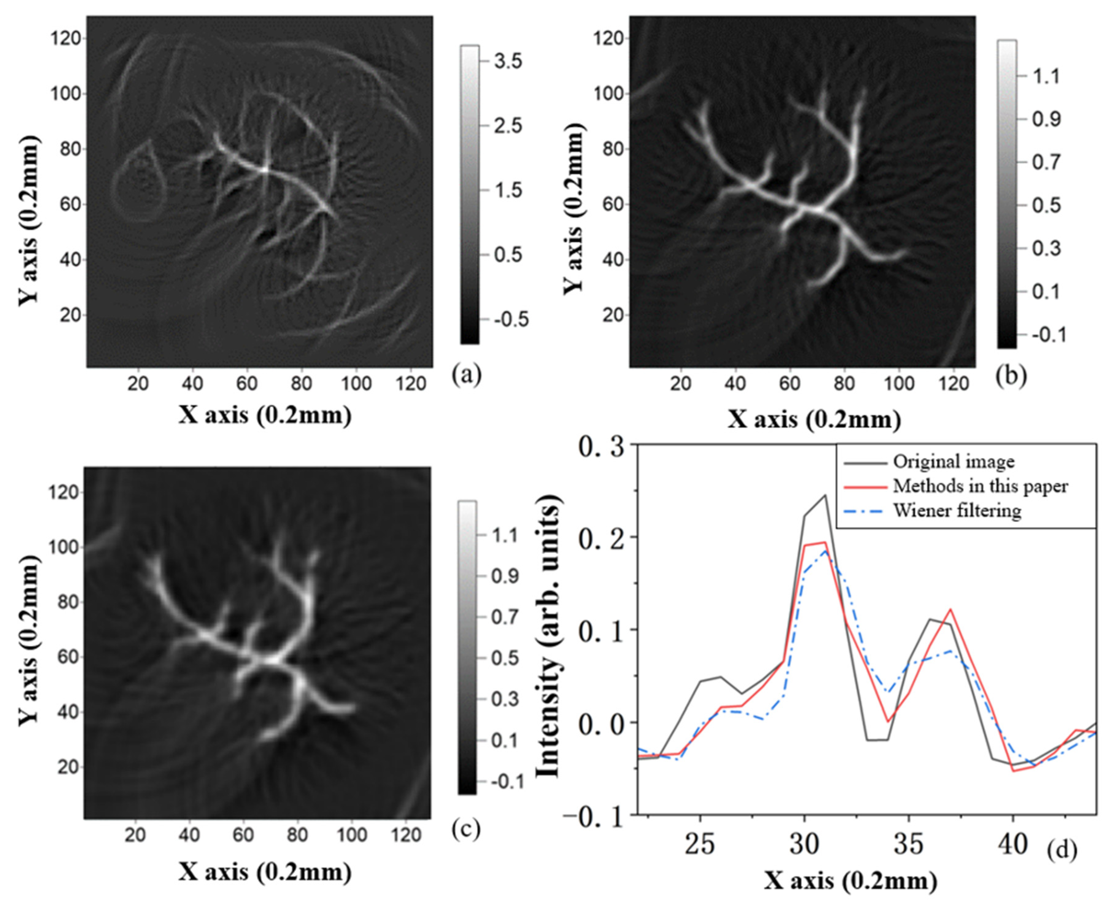
4.4. Comparison with Classical Wiener Filtering

Finally, the method used in this paper is compared with the image before deblurring and Wiener filtering, and the reconstructed image as shown below is obtained. Figure 10a–c show the images reconstructed by the OPAS affected by TIR (reconstructed using time-reversal algorithm (TRA)), respectively, and the deconvolution algorithm in this paper obtains the reconstructed images after PAPS and the reconstructed images processed using Wiener filtering. As can be seen from Figure 10a, although the shape of the blood vessels can be seen in general, there are many interfering factors in the image. We can feel the effect of TIR on the image quality because there are many artefacts around the image, and it is difficult to see the details of the blood vessels in the image. As can be seen in Figure 10c, the Wiener filter image has eliminated some of the impulse responses, and the complete image of the vascular model can be seen, but the details in the image are still difficult to discern. In Figure 10b, the image obtained by the method used in this paper has a great improvement in sharpness compared to Wiener filtering. There is a significant reduction in artefacts around the image, with clearer details of the vessel model and sharper edges, indicating improved image resolution.

Figure 10d shows the curve from the 22nd to the 44th pixel of the data projected by the No. 1 transducer for a more intuitive comparison. Through the comparison of the images, it can be seen that the pixel values of the method used in this paper are closer to the original images than those of the Wiener filter. In contrast, the pixel values of the Wiener filter are slightly deviated from the original image, resulting in blurring of the edges. This proves that the problem of poor image quality due to TIR interference is significantly improved by the algorithm used in this paper. The algorithm can be used to solve the TIR of the transducer, thereby eliminating its influence on image clarity and improving image quality.

5. Simulation of OPAS with Noise

Gaussian noise with a signal-to-noise ratio (SNR) of 40 is added to the previous simulation data, and the improved algorithm is used for the simulation, so that the algorithm can be effectively applied to the experiment. We selected three transducers, the No. 1 transducer and two transducers rotated 2.25° and 4.5° clockwise around the center of the reconstructed region from the No. 1 transducer position. The image of the eigenvalue solved by the first step of the algorithm is shown in Figure 11a. Apart from the last, particularly small eigenvalue, the other eigenvalues generally show steady decay.

We first discard the two smallest eigenvalues and then enlarge the eigenvalues with slightly obvious changes in the tail of the image to obtain Figure 11b. It can be seen that the points with large jumps are between the 25th and 26th and between the 33rd and 34th. The difference between the 25th and 26th eigenvalue is −0.27 and the difference between the 33rd and 34th eigenvalue is −0.23. Therefore, in comparison, the 26th eigenvalue is the point with the greater jump compared to the other eigenvalues (after dropping the two smallest eigenvalues). This allows us to assume that the minimum number of eigenvalues is 12, i.e., L = 12.

Then, the second step of the improved algorithm is used to continue the calculation. At this point, the solution result contains only one minimum eigenvalue, and the eigenvector corresponding to this minimum eigenvalue is the factor that affects the quality of the photoacoustic image. Decomposing the feature vector into three groups, then solving by LS algorithm, can obtain PAPS after noise removal, as shown in Figure 12. Figure 12a shows OPAS affected by noise and TIR, and Figure 12b shows PAPS after noise removal after processing by the improved algorithm. After the noise has been removed, the lines of the PAPS images become smooth, and the influence of the noise is largely eliminated.

We reconstructed the OPAS data containing noise and TIR, and the PAPS data obtained after the improved algorithm, and obtained Figure 13a,b. We can see that the improved algorithm can effectively eliminate the noise and TIR effects. In Figure 13b, the lines of the blood vessel model in the image are obvious, the structure and details of the vascular model can be clearly seen. In terms of noise and TIR removal, the improved algorithm is very effective.

6. Conclusions

In this paper, an algorithm for solving TIR is proposed. The advantage of this algorithm is that TIR can be extracted directly from OPAS data. The PAPS is then restored to the point where it can recover the edges and fine details of the PA image. The results show that the algorithm can solve the problem of reconstructing image blur due to the TIR itself. Finding the PAPS makes it possible to obtain an accurate TIR suitable for PAI technology research. And it can eliminate the interference of the transducer TIR on the clarity of the reconstructed image by deconvolution and improve the quality of the reconstructed image. The PA image processed by the algorithm is no longer affected by the TIR. In order to save time in operation, it is also discussed that at least two transducer datapoints can be selected for calculation when solving TIR. However, in order to obtain an accurate TIR, the complete OPAS generated by the biological tissue should be selected for each transducer. Ensure the accuracy of calculation results while reducing calculation time. In the future, the algorithm perhaps will be more widely used in photoacoustic imaging technology.

References

1. Wang, L.V.; Hu, S. Photoacoustic Tomography: In Vivo Imaging from Organelles to Organs. Science 2012, 335, 1458–1462. [Google Scholar] [CrossRef] [PubMed]
2. Paltauf, G.; Nuster, R.; Frenz, M. Progress in biomedical photoacoustic imaging instrumentation toward clinical application. J. Appl. Phys. 2020, 128, 180907. [Google Scholar] [CrossRef]
3. Li, J.; Ma, Y.F.; Tao, Z.; Shung, K.K.; Zhu, B. Recent Advancements in Ultrasound Transducer: From Material Strategies to Biomedical Applications. BME Front. 2022, 2022. [Google Scholar] [CrossRef] [PubMed]
4. Roy, K.; Lee, J.E.-Y.; Lee, C. Thin-film PMUTs: A review of over 40 years of research. Microsyst. Nanoeng. 2023, 9. [Google Scholar] [CrossRef] [PubMed]
5. Herickhoff, C.D.; van Schaijk, R. cMUT technology developments. Z. Für Med. Phys. 2023, 33, 256–266. [Google Scholar] [CrossRef] [PubMed]
6. Oraevsky, A.A.; Savateeva, E.V.; Solomatin, S.V.; Karabutov, A.A.; Andreev, V.G.; Gatalica, Z.; Khamapirad, T.; Henrichs, P.M. Optoacoustic imaging of blood for visualization and diagnostics of breast cancer. Biomed. Optoacoust. 2002, 4618, 81–94. [Google Scholar]
7. Hoelen, C.G.A.; de Mul, F.F.M.; Pongers, R.; Dekker, A. Three-dimensional photoacoustic imaging of blood vessels in tissue. Opt. Lett. 1998, 23 8, 648–650. [Google Scholar] [CrossRef]
8. Siphanto, R.I.; Thumma, K.K.; Kolkman, R.G.M.; Leeuwen, T.G.v.; Mul, F.F.M.d.; Neck, J.W.v.; Adrichem, L.N.A.v.; Steenbergen, W. Serial noninvasive photoacoustic imaging of neovascularization in tumor angiogenesis. Opt. Express 2005, 13, 89–95. [Google Scholar] [CrossRef]
9. Wang, X.; Pang, Y.; Ku, G.; Xie, X.; Stoica, G.; Wang, L.V. Noninvasive laser-induced photoacoustic tomography for structural and functional in vivo imaging of the brain. Nat. Biotechnol. 2003, 21, 803–806. [Google Scholar] [CrossRef]
10. Xu, Y.; Wang, L.V. Rhesus monkey brain imaging through intact skull with thermoacoustic tomography. IEEE Trans. Ultrason. Ferroelectr. Freq. Control 2006, 53, 542–548. [Google Scholar]
11. Li, C.; Wang, L.V. Photoacoustic tomography of the mouse cerebral cortex with a high-numerical-aperture-based virtual point detector. J. Biomed. Opt. 2009, 14, 024047. [Google Scholar] [CrossRef] [PubMed]
12. Dangi, A.; Roy, K.; Agrawal, S.K.; Chen, H.; Ashok, A.; Wible, C.; Osman, M.; Pratap, R.; Kothapalli, S.-R. A modular approach to neonatal whole-brain photoacoustic imaging. In Photons Plus Ultrasound: Imaging and Sensing 2020; BiOS: Sydney, Australia, 2020. [Google Scholar]
13. Pramanik, M.; Ku, G.; Li, C.; Wang, L.V. Design and evaluation of a novel breast cancer detection system combining both thermoacoustic (TA) and photoacoustic (PA) tomography. Med. Phys. 2008, 35, 2218–2223. [Google Scholar] [CrossRef] [PubMed]
14. Ermilov, S.A.; Khamapirad, T.; Conjusteau, A.; Leonard, M.H.; Lacewell, R.D.; Mehta, K.; Miller, T.; Oraevsky, A.A. Laser optoacoustic imaging system for detection of breast cancer. J. Biomed. Opt. 2009, 14, 024007. [Google Scholar] [CrossRef] [PubMed]
15. Kruger, R.A.; Miller, K.D.; Reynolds, H.; Kiser, W.L.; Reinecke, D.R.; Kruger, G.A. Breast cancer in vivo: Contrast enhancement with thermoacoustic CT at 434 MHz-feasibility study. Radiology 2000, 216, 279–283. [Google Scholar] [CrossRef] [PubMed]
16. Manohar, S.; Vaartjes, S.; van Hespen, J.C.G.; Klaase, J.M.; van den Engh, F.M.; Steenbergen, W.; van Leeuwen, T.G. Initial results of in vivo non-invasive cancer imaging in the human breast using near-infrared photoacoustics. Opt. Express 2007, 15, 12277–12285. [Google Scholar] [CrossRef]
17. Piras, D.; Xia, W.; Steenbergen, W.; van Leeuwen, T.G.; Manohar, S. Photoacoustic Imaging of the Breast Using the Twente Photoacoustic Mammoscope: Present Status and Future Perspectives. IEEE J. Sel. Top. Quantum Electron. 2010, 16, 730–739. [Google Scholar] [CrossRef]
18. Song, K.H.; Stein, E.W.; Margenthaler, J.A.; Wang, L.V. Noninvasive photoacoustic identification of sentinel lymph nodes containing methylene blue in vivo in a rat model. J. Biomed. Opt. 2008, 13, 054033. [Google Scholar] [CrossRef]
19. Erpelding, T.N.; Kim, C.; Pramanik, M.; Janković, L.; Maslov, K.; Guo, Z.; Margenthaler, J.A.; Pashley, M.D.; Wang, L.V. Sentinel lymph nodes in the rat: Noninvasive photoacoustic and US imaging with a clinical US system. Radiology 2010, 256, 102–110. [Google Scholar] [CrossRef]
20. Pan, D.; Pramanik, M.; Senpan, A.; Ghosh, S.; Wickline, S.A.; Wang, L.V.; Lanza, G.M. Near infrared photoacoustic detection of sentinel lymph nodes with gold nanobeacons. Biomaterials 2010, 31, 4088–4093. [Google Scholar] [CrossRef]
21. Pramanik, M.; Song, K.H.; Swierczewska, M.; Green, D.E.; Sitharaman, B.; Wang, L.V. In vivo carbon nanotube-enhanced non-invasive photoacoustic mapping of the sentinel lymph node. Phys. Med. Biol. 2009, 54, 3291–3301. [Google Scholar] [CrossRef]
22. Lu, Q.-B.; Liu, T.; Ding, L.; Lu, M.-H.; Zhu, J.; Chen, Y.-F. Probing the Spatial Impulse Response of Ultrahigh-Frequency Ultrasonic Transducers with Photoacoustic Waves. Phys. Rev. Appl. 2020, 14, 034026. [Google Scholar] [CrossRef]
23. Seeger, M.R.; Soliman, D.; Aguirre, J.; Diot, G.; Wierzbowski, J.; Ntziachristos, V. Pushing the boundaries of optoacoustic microscopy by total impulse response characterization. Nat. Commun. 2020, 11, 2910. [Google Scholar] [CrossRef] [PubMed]
24. Ku, G.; Wang, X.; Stoica, G.; Wang, L.V. Multiple-bandwidth photoacoustic tomography. Phys. Med. Biol. 2004, 49, 1329–1338. [Google Scholar] [CrossRef] [PubMed]
25. Sheu, Y.-L.; Chou, C.-Y.; Hsieh, B.-Y.; Li, P.-C. Image reconstruction in intravascular photoacoustic imaging. IEEE Trans. Ultrason. Ferroelectr. Freq. Control 2011, 58, 2067–2077. [Google Scholar] [CrossRef] [PubMed]
26. Yang, C.; Jiao, Y.; Jian, X.; Cui, Y. Image Deconvolution with Hybrid Reweighted Adaptive Total Variation (HRATV) for Optoacoustic Tomography. Photonics 2021, 8, 25. [Google Scholar] [CrossRef]
27. Rathi, N.; Sinha, S.; Chinni, B.; Dogra, V.S.; Rao, N. Computation of Photoacoustic Absorber Size from Deconvolved Photoacoustic Signal Using Estimated System Impulse Response. Ultrason. Imaging 2021, 43, 46–56. [Google Scholar] [CrossRef]
28. Kruger, R.A.; Reinecke, D.R.; Kruger, G.A. Thermoacoustic computed tomography—Technical considerations. Med. Phys. 1999, 26, 1832–1837. [Google Scholar] [CrossRef]
29. Xu, M.; Wang, L.V. Time-domain reconstruction for thermoacoustic tomography in a spherical geometry. IEEE Trans. Med. Imaging 2002, 21, 814–822. [Google Scholar]
30. Wang, Y.; Xing, D.; Zeng, Y.; Chen, Q. Photoacoustic imaging with deconvolution algorithm. Phys. Med. Biol. 2004, 49, 3117–3124. [Google Scholar] [CrossRef]
31. Lu, T.; Mao, H. Deconvolution Algorithm with LTI Wiener Filter in Photoacousic Tomography. In Proceedings of the 2009 Symposium on Photonics and Optoelectronics, Wuhan, China, 14–16 August 2009; pp. 1–4. [Google Scholar]
32. Qi, L.; Wu, J.; Li, X.; Zhang, S.; Huang, S.; Feng, Q.; Chen, W. Photoacoustic Tomography Image Restoration With Measured Spatially Variant Point Spread Functions. IEEE Trans. Med. Imaging 2021, 40, 2318–2328. [Google Scholar] [CrossRef]
33. Bravo-Miranda, C.A.; Gonzalez-Vega, A.; Gutiérrez-Juárez, G. On the sensor influence in photoacoustic signal produced by point-like source. Biomed. Opt. 2013, 8581, 858144. [Google Scholar]
34. Bravo-Miranda, C.A.; Gonzalez-Vega, A.; Gutiérrez-Juárez, G. Influence of the size, geometry and temporal response of the finite piezoelectric sensor on the photoacoustic signal: The case of the point-like source. Appl. Phys. B 2014, 115, 471–482. [Google Scholar] [CrossRef]
35. Bravo-Miranda, C.A.; Gonzalez-Vega, A.; Gutiérrez-Juárez, G. Dependence of photoacoustic signal generation on the transducer and source type. Biomed. Opt. 2014. [Google Scholar]
36. Rietsch, E. Euclid and the art of wavelet estimation, Part I: Basic algorithm for noise-free data. Geophysics 1997, 62, 1931–1938. [Google Scholar] [CrossRef]
37. Koay, C.G.; Chang, L.-C.; Carew, J.D.; Pierpaoli, C.; Basser, P.J. A unifying theoretical and algorithmic framework for least squares methods of estimation in diffusion tensor imaging. J. Magn. Reson. 2006, 182, 115–125. [Google Scholar] [CrossRef]
38. Veraart, J.; Sijbers, J.; Sunaert, S.; Leemans, A.; Jeurissen, B. Weighted linear least squares estimation of diffusion MRI parameters: Strengths, limitations, and pitfalls. NeuroImage 2013, 81, 335–346. [Google Scholar] [CrossRef]
39. Treeby, B.E.; Cox, B.T. k-Wave: MATLAB toolbox for the simulation and reconstruction of photoacoustic wave fields. J. Biomed. Opt. 2010, 15, 021314. [Google Scholar] [CrossRef] [PubMed]
Figure 1. In this paper, the use of the blood vessel grid model, the distribution of the sensor position, and IRT. (a) Describe the photoacoustic data acquisition geometry diagram. (b) Vascular mesh model in the K-Wave toolbox. (c) The hypothesized TIR is in this paper.
Applsci 14 00920 g001
Figure 2. The result obtained by the algorithm. (a) The relative size of 339 eigenvalues. (b) The relative size of the 40 eigenvalues after recalculating the eigenvalues. (c) Comparison of the calculated PAPS from one of the transducers with its original PAPS.
Applsci 14 00920 g002
Figure 3. LS algorithm calculates the TIR.
Applsci 14 00920 g003
Figure 4. TIR was obtained from 2 transducers’ data.
Applsci 14 00920 g004
Figure 5. It uses two transducer data to obtain the PAPS.
Applsci 14 00920 g005
Figure 6. Results after the algorithm is corrected. (a) Corrected the PAPS. (b) The TIR is calculated after correcting the PAPS.
Applsci 14 00920 g006
Figure 7. (a) The calculated PAPS when the OPAS is 100 signal lengths is compared to the original PAPS. (b) The calculated PAPS when the OPAS is 200 signal lengths is compared to the original PAPS.
Applsci 14 00920 g007
Figure 8. TIR results with an OPAS length of 100. (a) The TIR length is 30. (b) The TIR length is 40.
Applsci 14 00920 g008
Figure 9. TIR results with an OPAS length of 200. (a) The TIR length is 30. (b) The TIR length is 40.
Applsci 14 00920 g009
Figure 10. (a) The OPAS image is reconstructed using TRA. (b) A reconstructed image of the PAPS. (c) The image reconstructed by the Wiener filter algorithm. (d) Comparison of the pixel values of the two algorithms with the original image.
Applsci 14 00920 g010
Figure 11. (a) Eigenvalue images of OPAS with noise. (b) Enlarged end of figure (a) (omit the last two points).
Applsci 14 00920 g011
Figure 12. (a) OPAS images with noise and TIR. (b) The PAPS obtained by using the improved algorithm.
Applsci 14 00920 g012
Figure 13. Reconstructed image. (a) The OPAS image is reconstructed using TRA. (b) Reconstructed image with improved algorithm.
Applsci 14 00920 g013
Disclaimer/Publisher’s Note: The statements, opinions and data contained in all publications are solely those of the individual author(s) and contributor(s) and not of MDPI and/or the editor(s). MDPI and/or the editor(s) disclaim responsibility for any injury to people or property resulting from any ideas, methods, instructions or products referred to in the content.