Abstract
Graph mining has emerged as a significant field of research with applications spanning multiple domains, including marketing, corruption analysis, business, and politics. The exploration of knowledge within graphs has garnered considerable attention due to the exponential growth of graph-modeled data and its potential in applications where data relationships are a crucial component, and potentially being even more important than the data themselves. However, the increasing use of graphs for data storing and modeling presents unique challenges that have prompted advancements in graph mining algorithms, data modeling and storage, query languages for graph databases, and data visualization techniques. Despite there being various methodologies for data analysis, they predominantly focus on structured data and may not be optimally suited for highly connected data. Accordingly, this work introduces a novel methodology specifically tailored for knowledge discovery in labeled and heterogeneous graphs (KDG), and it presents three case studies demonstrating its successful application in addressing various challenges across different application domains.
1. Introduction
The field of graph mining has witnessed a surge in popularity in recent years, primarily fueled by the exponential growth of data that can be effectively represented as graphs and its wide range of application areas. This has led to the rise of graph databases such as Neo4J, AllegroGraph, and OrientDB [1], which offer robust platforms for modeling and storing data as interconnected nodes and relationships. Leveraging these databases, researchers and practitioners can apply advanced graph mining algorithms to accomplish various tasks, including community analysis, centrality identification, pathfinding, and exploring structural patterns. In various application domains, such as Business Information Systems [2], Financial Crime Detection Systems [3], Transport Information Systems [4], and Recommendation Systems [5], graph databases have gained widespread acceptance. However, relying solely on graph databases is insufficient. A comprehensive methodology is necessary to establish the task and stages for effectively conducting information analysis and extracting valuable insights.
This paper reviews existing work of graph mining and presents the frameworks and methodologies most used for knowledge discovery, such as KDD [6], CRISP-DM [7], and SEMMA [8]. We describe the required tasks for deriving value from large graphs absent in methodologies and frameworks used in the literature. Finally, based on KDD, CRISP-DM, and the required tasks for graph mining, we propose a new methodology for knowledge discovery in graphs.
The contributions of the paper are the following:
- A new and specific methodology named KDG (knowledge discovery in graphs) to guide users to find insights from data represented as graphs.
- Three use cases applying the proposed methodology.
The remainder of the paper is structured as follows. Section 2 provides an overview of the frameworks and methodologies employed in data mining, including the processes, tools, visualization techniques, and graph analysis algorithms that have emerged in the past two decades. Section 3 introduces the related concepts that are employed throughout the paper. Section 4 presents our methodology for knowledge discovery in graphs, outlining its essential components and task. Then, in Section 5, we showcase the application of this methodology through three different use cases. Finally, in Section 6, we discuss our findings and avenues for future research.
2. Related Work
Graph mining refers to the set of tools and algorithms used to model graphs that match patterns found in the real world, analyze graph properties, and predict how structures and properties of a given graph might affect some applications [9]. We reviewed works in the graph mining field over the last two decades, from frameworks and methodologies for project development to modeling tools and algorithms for graph analysis. The following section provides an overview of the commonly employed methodologies and data mining frameworks utilized for knowledge discovery in graphs.
2.1. Frameworks and Methodologies
Fayyad et al. [6] defined knowledge discovery in databases (KDD) as a process that identifies useful, valuable, and understandable patterns in data. They addressed how algorithms can be scaled to work well on massive datasets and how they can be visualized and interpreted. In addition, they also included how human–machine interactions can be modeled and supported. In the KDD framework, data mining is a singular step within the process, where properly preprocessed data are transformed into patterns that yield valuable knowledge. However, it is important to note that several methodologies developed after KDD, such as CRISP-DM [7] and SEMMA [8], use data mining as a synonym for KDD.
CRISP-DM is widely recognized as the methodology for most proposals for data mining process models as data science has evolved. This methodology restates the steps of the original KDD proposal into business understanding, data understanding, data preparation, modeling, evaluation, and implementation. On the other hand, SEMMA methodology was proposed by SAS [8] and stands for Sample, Explore, Modify, Model, and Assess. This methodology focuses primarily on the technical aspects of data mining product development and is strongly tied to the SAS data miner. A significant difference between SEMMA and previous methodologies is the prerequisite of having and understanding the business requirements and databases.
CRISP-DM, SEMMA, and other related methodologies such as ASUM-DM [10], CASP-DM [11], FMDS [12], and TDSP [13] are based on a goal-oriented perspective, dealing with processes, tasks, and roles. These methodologies were developed mainly focused on data mining processes with relatively clear business objectives. Furthermore, they primarily deal with structured data, which may originate from flat files or be obtained through querying relational databases. However, currently in the context of big data and data science, the great diversity of information sources, the amount of data, the heterogeneity of the data, and the complexity of the problems represent a challenge for classical methodologies.
In recent years, new proposals have emerged to bridge the gap between classical methodologies and the complexity of current problems. Martínez-Plumed et al. [14] propose a data trajectory model (DST) and categorize data science projects into goal-directed, exploratory, and data management. Their model extends CRISP-DM, including six exploratory activities focused on the goal, data source, data value, results, narrative, and product. Although DST is a proposal that may reduce the gap between data mining methodologies and data science projects, the proposal is limited to proposing exploratory activities for tabular data, which it describes in its use cases. Studer et al. [15] proposed a process model for developing machine learning applications.
Regarding frameworks, various proposals have emerged focused on different phases of knowledge discovery in graphs, for example, business understanding [16], data modeling [17], graph mining [18,19,20], graph visualization [21,22], and evaluation [23,24].
Some proposals are focused on how to model realistic graphs that match the patterns found in real-world graphs. Shrivastava et al. [25] proposed a graph mining framework that captures entities and relations between entities from different data sources. Their framework offers a comprehensive approach with five modules covering graph preprocessing, graph database, dense substructure extraction, frequent substructure discovery, and graph visualization. However, it lacks adequate addressing of the business goals and the evaluation process within the scope.
Nasiri et al. [26] presented a framework with two modeling components: context modeling and analytics design alternatives modeling. The first is to justify the need for predictive analytics within the organizational context. It extends the business intelligence model (BIM) [16], and the second is to identify the requirements for adapting the framework presented [27], but it lacks adequate addressing of considering the valuable insights that can be extracted from graph data. Therefore, integrating graph databases into the framework could enhance its effectiveness in uncovering hidden patterns and relationships within the data.
Data modeling as a graph and its analysis found a good area of application in social networks. Authors such as Kumar [17] and Schroeder [28] have developed frameworks that focus on social networks such as Twitter. Kumar et al. [17] proposed a framework for analyzing social networks. They used natural language processing to isolate node features and meta-data for edges. The main phases of the framework are data acquisition, preprocessing, multi-attributed graph creation, the transformation of the multi-attributed graph into a similarity graph, and clustering. However, the scope is limited to social networks. Schroeder et al. [28] presented a framework for collecting graph structures of follower networks, posts, and profiles on the social network Twitter. The goal is to detect social bots by analyzing graph-structured data.
2.2. Tools and Algorithms for Graph Analysis
In addition to proposal methodologies and frameworks, relevant works focus on graph mining algorithms with different aims, such as summarizing and visualizing graphs, performing aggregation operations on the data, searching for substructures in the graph, automatic construction of graphs, and developing proposals to optimize operations performed on the graphs.
Some works in the literature focus on analyzing subgraphs and transforming the graph topology. Qiao [29] proposesd a parallel frequent subgraph mining algorithm in a single large graph using Spark. The proposal employs a heuristic search strategy, load balancing, research pruning, and top-down pruning in the support. Qiao also proposed a two-phase framework. In the first phase, the parallel subgraph extension uses a strategy that generates all subgraphs in parallel. In the second phase, he uses a similar support evaluation method for finding subgraph isomorphisms. Zhang [30] proposed a framework for the weighted meta-graph-based classification of heterogeneous information networks. The core is an algorithm that iterative classifies objects in heterogeneous information networks to capture the information hidden in the semantics and structure of the graph. Lee et al. [31] proposed a method for extracting frequent subgraphs while maintaining semantic information and considering scalability in large-scale graphs. The generated semantic information includes frequency counts for tasks such as rating prediction or recommendation.
Pienta et al. proposed Vigor [18], an interactive tool for graph exploration that includes both bottom-up and top-down sensemaking for analysts, facilitating their review of subgraphs through a summarization process. This proposal provides valuable contributions to the field of graph exploration. However, there is an opportunity to explore further the business requirements. Additionally, Dunne and Shneiderman’s work [32] focused on improving graph visualization through motif simplification, which replaces common patterns of nodes and links with compact and meaningful glyphs, further enhancing graph exploration.
Yin and Hong investigated the problem of aggregation on different types of nodes and relations by proposing a function bases on graph entropy to measure the similarities of nodes. They also proved that the aggregation problem based on the functions is NP-hard and proposes a heuristic algorithm to perform aggregation, including informational and structural aspects. Despite the study’s limited scope of the algorithm proposal, their work is significant in addressing the fundamental operation of performing aggregations on data stored in graph nodes.
Searching, processing, and visualizing subgraphs can be a task that requires many computational resources. For this reason, authors such as Bok et al. [19] have developed proposals on enhancing subgraph accessibility. They propose a two-level caching strategy that caches subgraphs that are likely to be accessed depending on the usage pattern of subgraphs. Their proposal prevents the caching of low-usage subgraphs and frequent subgraph replacement in the memory. One of their proposal’s main applications is enabling the processing and analyzing of large graph queries in computing environments with small memory.
In the last decade, various proposals have emerged that focus on different phases of knowledge discovery in graph databases. These proposals encompass areas such as business understanding [16], data modeling [17], graph mining [18,19,20], graph visualization [21,22], and evaluation [23,24].
The methodologies, frameworks, tools, and algorithms mentioned in Section 2.1 and Section 2.2 have demonstrated their value, but there is still a need for a comprehensive methodology that incorporates existing advancements and algorithms. Such a methodology should provide a detailed and specific guide for analyzing related data using graphs, addressing the diverse tasks involved in knowledge discovery. By incorporating these elements, the users will have clear directions to maximize the potential of graphs in their data analysis projects.
Adopting a comprehensive methodology encompassing critical tasks is imperative to leverage the knowledge embedded in data relationships. These tasks involve modifying a graph by applying rules or operations to its nodes and edges and incorporating new structural attributes that before do not exist in nodes or relations. Additionally, the visual representation of graphs and networks plays a vital role in this process. Creating visual depictions of graphs allows users to identify patterns, anomalies, and trends within complex datasets, thereby attaining a deeper understanding of the underlying information.
The methodology under discussion provides a detailed and specific guide for analyzing related data using graphs. It encompasses a wide range of operations and tasks that can be performed, offering a comprehensive array of options. Furthermore, it presents a coherent order of stages and steps, serving as a valuable reference for conducting thorough exploration and analysis in a structured manner. The methodology emphasizes effective modeling and analysis of information using graphs while ensuring flexibility in choosing tools and algorithms. By following this guide, the users will receive clear directions to maximize the potential of graphs in their data analysis projects.
3. Related Concepts
In this section, we introduce the principal notions of graphs needed to understand the proposed work. For further information, we refer to [33,34].
3.1. Graphs
A graph is a mathematical structure consisting of elements named vertices or nodes, connected by links named edges. A vertex represents an entity that can be any object, such as people, products, or cities. An edge represents the relationship between two entities. Some common applications of graphs include social networks, where vertexes are people and the edges represent friendship or other relationships between people, and transportation networks, where vertexes are places (e.g., bus stops and airports) and the edges are the paths between those places.
According to the nature of the problem, we can model the data using different types of graphs, whether the relationships between vertexes are bidirectional the graph is known as an undirected graph; hence, the edge is represented as a straight line. Otherwise, the graph is known as a directed graph and the edge is represented as an arrow. In this work, we focus on graphs where the nodes and edges might have one or more associated attributes, named the labeled graph. Moreover, we can use nodes or edges of different entities and attributes known as the heterogeneous graph in addition to homogeneous graphs, where nodes and edges are of the same type and attributes.
3.2. Graph Structure
In order to analyze the graphs, it is useful to consider the structural information of the graphs, and therefore, it is important to introduce some basic notions as follows.
Graph topology is the arrangement and the form in which nodes are connected. Through the topology analysis, we could find some important features for the graph analysis, such as the node’s degree, which refers to the number of relationships of a node. In-degree refers to the relationships that enter a node, and out-degree refers to the relationships that leave a node. In undirected graphs, in-degree, out-degree, and degree have the same value.
Nodes’ centrality is used to identify essential or central nodes in a network. A community is used to describe a cluster or a set of highly connected nodes within a network. Similarity is a form to measure or compare how similar two different nodes are in a network considering their relationships, structural information, or attributes. Path is a sequence of nodes that are connected throughout the network.
Another important concept to understand the herein proposed work is the subgraph, a portion of the original graph consisting of a subset of selected nodes and edges, which reduces the model’s size, and therefore, the analysis’s complexity. A subgraph might be the result of applying a filter. Two useful operations for analyzing a graph structure are filtering and summarization. A filter can be a helpful tool to select or show a subset of nodes or relationships that meet certain conditions or criteria. Using filters can reduce the size and complexity of the graph and facilitate the analysis and visualization of important information. Filters can be applied based on attributes, degree, community, weight, or distance, among others. Structural attributes of a graph are characteristics that describe the topology. Some examples of structural attributes are degree, community, and path, among others. Graph summarization is a process that allows for a more compact representation of the original graph to facilitate the analysis and understanding of complex graphs. Various algorithms can be used to summarize graphs, by grouping nodes or relationships based on specific attributes or types of entities to present a more concise version of the complete graph.
3.3. Graph Visualization
Graph modeling creates an abstract and structured representation of elements represented by nodes and relationships represented by edges to analyze complex systems in computer science, social sciences, engineering, and more. The graph model can be displayed using different layouts. A layout refers to the form and position in which the nodes and relationships of a graph are represented on a visualization plane. Various visualization algorithms aim to minimize the crossing or overlap of relationships and nodes. In the context of analysis and visualization, drill-down and roll-up operations are two techniques used to explore data hierarchically and obtain different levels of detail or summary. Drill-down involves breaking down data from a higher or more general level to a lower or more detailed level in a data hierarchy. Roll-up involves summarizing data from a lower or more detailed level to a higher or more general level.
Some problems, by their nature, require considering the graph’s evolution through time. In this case, we can analyze the graph by using a timeline, which is a graphical and sequential representation of events over time. It shows how nodes and relationships are positioned at specific moments and how they evolve.
4. Methodology Proposal
Analyzing large amounts of highly related information is complex, and sometimes it is required to visualize it in a summarized way. Some examples are product recommendations, fraud detection, analysis of relationships such as friendships, collaboration, co-authorship, lines of authority, influencer detection, logistics in the product supply chain, bill of materials, routing in a computer network, or finding roads.
We propose a methodology named KDG for knowledge discovery in graphs as a reference to extract, transform, load, process, model, visualize, and analyze highly connected information that can be represented by labeled and heterogeneous graphs; applying mining algorithms to discover new structural features useful to improve the analysis that supports decision making.
Our methodology provides a global overview of the stages that may be required in the knowledge discovery process modeled by graphs, which considers all possible tasks for exploring the information, identifying patterns, making recommendations by applying queries, using visualization tools, and solving questions, among others.
Figure 1 illustrates the methodology of our approach that comprises six stages: (1) Understanding the Analytical Process, (2) Graph Building, (3) Graph Mining, (4) Graph Transformation, (5) Graph Visualization, and (6) Evaluation. Each stage contains several tasks. The user can choose to accomplish all the tasks in each stage or, at a minimum, focus on those highlighted explicitly in bold within the figure, as these represent the essential tasks needed for the methodology.
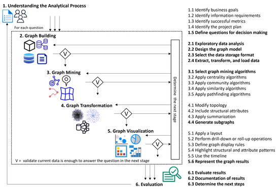
Figure 1.
The methodology for knowledge discovery in labeled and heterogeneous graphs (KDG).
4.1. Stage 1: Understanding the Analytical Process
The aim of this stage is to establish a comprehensive understanding of all the steps involved in data analysis before undertaking any actions, analyses, or proceeding to subsequent stages within the methodology. Furthermore, it is essential to establish a cohesive guiding thread that will lead the user consistently throughout the entire application of the methodology.
This stage consists of five tasks: (1.1) Identify business goals, which consists of aligning the objectives of the analysis with the company’s mission and vision. These goals typically follow the SMART goal framework, which means they are specific, measurable, achievable, relevant, and time-bound; more information can be found at [35]. (1.2) Identify information requirements which are concrete and feasible, outlining the necessary functionalities. Some examples are: using a specific technology, algorithm, or tool, data confidentiality, and using specific data sources. If the reader wants to delve into the information required for requirements, they can refer to [36]. (1.3) Identify successful metrics for getting objective data that help users to discover improvement areas and ensure that the project progress is according to the established goals. It can be quantitative or qualitative measures used to asses and gauge various aspects of a project, its progress, and its performance. Some examples of metrics are cost, time, and quality. If the reader wants to delve into the information required for the metrics, they can refer to [37,38]. (1.4) Identify the project plan is a guiding document for all stakeholders, providing clear direction. It defines the project’s scope, duration, required activities, and agreed-upon deliverables. The essential components of a project plan include the overall business vision, project scope, objectives to be achieved, team members involved, assigned roles and responsibilities, agreed-upon deliverables, activity schedule, associated budget, and written approval from the project sponsor. If the reader wants to delve into the information required for the project plan, they can refer to [39]. (1.5) Define questions for decision making. Their primary objective is facilitating the gathering of relevant information, evaluating available options, and considering factors influencing well-informed and effective decision making. These questions are applicable in personal and professional contexts, addressing specific dilemmas and contributing to resolving highly significant problems. They are characterized by their reflective nature and precise focus, centering on goals, alternatives, consequences, and personal values, often necessitating deep contemplation. If the reader wants to go deeper into the appropriate way to define questions for decision making, they can refer to [40,41]. The questions that are particularly useful for the analysis have to take into account the highly connected information and are concise enough to obtain a clear answer as an output for the analysis. Some examples of questions are: how are the data related to each other? Are there some paths between specific elements? Which are the groups of most related or similar elements? Which are the elements with more connections in the network? What are the possible new connections between elements based on hidden data patterns? How similar is one element to another in terms of its connections? It is important to note that these questions are the output of this stage, and stages 2 to 5 are performed for each question.
4.2. Stage 2: Graph Building
The aim of this stage is to create a graph model that considers the questions formulated in the previous stage and validate that the data is sufficient to address the questions. Additionally, it is essential to implement this graph model within a suitable data storage medium.
This stage consists of four tasks: (2.1) Exploratory Data Analysis, consisting of analyzing the available information by applying one or more of the following options: statistics, visualization, data aggregations, and identification of missing or corrupted data. This exploration and understanding of the data occur early in the process, preceding more in-depth data analysis. In the context of graph building, the objective of this activity is to identify the entities, properties, and their relationship useful to answer each question defined in the previous stage. For guidance in the exploratory data analysis (EDA), the reader can refer to [42,43], and for a review, a comparative study of four methods employed in EDA, they can refer to [44]. (2.2) Graph Model Design defines which data will be represented as nodes, establishes the relationships between them, and defines the attributes associated with each element. It is possible to design homogeneous or heterogeneous graphs, as well as labeled or not labeled and directed or indirected graphs. For guidance in the model process, the reader can refer to [34,45,46]. (2.3) Data Storage Formats Selection, which involves choosing the technology to store it in graph databases, such as relational, columns, key-value, documents, graphs, or any other type of file format. To fully harness the analytical potential of graph analysis, opting for a graph database is recommended but not obligatory. The reader can refer to [47] for guidance in this selection process. Some examples are NEO4J, TigerGraph, JSON files, MongoDB, and Apache Cassandra. Finally, (2.4) Extract, Transform, and Load Data involves acquiring data from diverse sources, including databases, spreadsheets, flat files, or web services. Data are collected from various origins and brought into a staging area for subsequent processing. Throughout the transformation phase, the data undergoes cleansing, formatting, and restructuring to align with the graph’s requirements. Ultimately, the refined and transformed data are loaded into the storage media. The reader can refer to [48,49,50] for guidance in this task. Examples of technologies that support extract, transform, and load tasks include Kettle Pentaho, AWS Glue, Knime, and Apache Spark.
The outcome of this stage is the successful implementation of the graph in the selected data storage format.
4.3. Stage 3: Graph Mining
Graph Mining is a powerful technique that allows for the analysis of various properties of graphs, prediction of graph structures and relationships, and modeling patterns found in real-world graphs [9]. This stage focuses on applying centrality, similarity, and community algorithms, as well as path search algorithms, based on the specific questions to answer. In certain instances, applying multiple algorithms to fully understand and analyze the graph may be necessary.
This stage consists of five tasks: (3.1) Select Graph Mining Algorithms, which can help users analyze and extract information from graph structures, such as social networks, corruption networks, and transportation systems. Depending on the specific context, users can apply centrality algorithms to pinpoint the most influential nodes, employ community algorithms to gain insights into potential node groupings, utilize similarity algorithms to assess node similarities based on their relationships or utilize pathfinding algorithms to ascertain the shortest or most advantageous routes between two or more nodes. For example, we could utilize a community algorithm to find similar products that can be recommended as a bundle, employ a route search algorithm to determine the shortest path between two points in different cities, deploy a centrality algorithm to locate a Facebook friend with the highest number of likes on their posts, or utilize a similarity algorithm to uncover alternative suppliers for products already in stock at a store. The reader can refer to [51] for guidance in this task. (3.2) Apply Centrality Algorithms plays an essential role in network analysis by allowing the evaluation and ranking of nodes based on their influence and importance. These algorithms are valid for the identification of influential nodes, the detection of opinion leaders, and the analysis of network structure. In essence, they provide a measure of the closeness or distance of a node to other nodes in the graph, which is essential for understanding the dynamics and impact of elements in a given network. Some examples are Degree Centrality, Betweenness Centrality, Closeness Centrality, and PageRank. The reader can refer to [52] for guidance in this task. (3.3) Apply Community Algorithms to delineate clusters or communities of nodes within a graph. These clusters comprise nodes that exhibit stronger connections among themselves than with nodes external to their respective groupings. Community algorithms look for patterns in node connectivity to identify these groups and can help understand how nodes are organized in a graph. Such algorithms find pertinent applications in identifying communities within social networks or detecting cohorts of users who exhibit shared interests on digital platforms. Some examples are Louvain, Label Propagation, Weakly Connected Components, Strongly Connected Components, Triangle Count, and K-1 Coloring. The reader can refer to [53] for guidance in this task. (3.4) Apply Similarity Algorithms quantifies and contrasts the structural similarity among distinct nodes, graphs, or subgraphs. These algorithms enable the assessment of the extent to which two graphs resemble each other regarding their structure, patterns, and interconnections among nodes. Some examples are Node Similarity, Jaccard Index, and K-Nearest Neighbors. The reader can refer to [54] for guidance in this task. (3.5) Apply Pathfinding Algorithms determines the shortest or most optimal route between two specific points on a graph or map. These algorithms find application in diverse domains, including GPS navigation systems, where they enable efficient route planning, video games for character movement, and transportation networks for optimizing package delivery routes. These algorithms employ search techniques and heuristics to identify the most favorable path, ensuring an efficient solution. Some examples are Dijkstra, Shortest Path, Breadth Search, Depth Seach, and Random Walk. The reader can refer to [55] for guidance in this task.
The outputs of the Graph Mining stage are helpful for further analysis. One of the key outcomes is the generation of information to create new structural attributes that provide additional insights into the graph’s properties. These attributes can be utilized for graph summarization, which helps reduce the complexity of the graph by creating higher-level abstractions and facilitating a more comprehensive understanding of the underlying patterns and structures. Additionally, the newly derived attributes can be used to address some of the initial questions that drove the analysis, providing valuable insights and answers.
4.4. Stage 4: Graph Transformation
The aim of this stage is to incorporate new attributes, nodes, or edges into the original graph, selecting subgraphs or executing queries to address the questions formulated in the initial phase.
This stage consists of four tasks guided by the questions defined in stage 1: (4.1) Modify Topology, which can improve the graph’s representation, enhancing the support for its analytical process. This task becomes necessary when the nodes or relationships initially present in the graph are insufficient to address the analysis questions. One example is to add new relationships for all product nodes purchased together. The reader can refer to [56] for guidance in this task. (4.2) Include Structural Attributes, which provides additional information in nodes and relationship attributes for a more comprehensive understanding of the graph’s structure to enhance the analysis. Examples encompass the integration of attributes such as degree centrality, PageRank centrality, Louvain community, and Jaccard similarity into node attributes, as well as including the Dijkstra path as relationship attributes. The reader can refer to [52] for guidance in this task. (4.3) Apply Summarization, which is useful to reduce the graph’s complexity by creating higher-level abstractions, allowing users to gain insights and identify patterns more quickly by grouping nodes, relationships, or both. For example, the graph can be summarized using attributes such as degree centrality, Louvain community, or other relevant measures. The reader can refer to [57] for guidance in this task. (4.4) Generate Subgraphs, which contains filtered and modified elements from the original graph, structural attributes, and summarization results. Each subgraph serves as a focused representation of the original graph, tailored to meet the specific analytical requirements of the users. Examples include the overall graph structure, a homogeneous graph, and specific nodes of interest. The reader can refer to [58] for guidance in this task.
The result of this stage consists of one or more subgraphs or graphs with nodes or edges with new attributes.
4.5. Stage 5: Graph Visualization
The core of the visualization stage lies in choosing appropriate representations of the graph to support answering the questions defined in stage 1. Users can choose several visualization forms, such as tables, networks, or graphics.
This stage has a strong dependence on the previous stages. We contemplate that there may be multiple iterations between the visualization stage and stage 1, 2, and 3. Allowing the incorporation of the results of previous tasks such as topological modifications, new structural attributes or other results of graph mining algorithms. Each alteration or transformation of the graph carries a visual representation that guides the ongoing analysis process.
This stage consists of six tasks:
(5.1) Apply Layout refers to configuring the shape, arrangement, and presentation of nodes, and their relationships within a graph. The objective is to enhance the legibility and comprehension of the network’s structure. Some examples are Force Atlas Layout, Circular Layout, Hierarchical Layout, and Tree Layout. The reader can refer to [59] for guidance in this task. (5.2) Perform Drill-down/Roll-up Operations are two approaches for navigating and scrutinizing hierarchical or layered data structures. They are useful for graph visualization and analysis, enabling the in-depth exploration of particulars or the synthesis of information within higher levels of the hierarchy. Moreover, they offer the capability to extract pertinent insights across varying levels of granularity or abstraction. Drill-down involves a comprehensive examination of the hierarchical data structure, commencing from an upper-tier perspective and progressively delving into finer levels of intricacy. Within the field of graph analysis, this entails the increasingly specific exploration of nodes and connections, starting from an initial node. For example, one can initiate a drill-down analysis at the category level, progressively descending to individual products. Conversely, roll-up refers to condensing data from lower tiers to upper levels within the hierarchy. In a graph, it might be necessary the combination or abstraction of nodes and relationships to present a broader or more top-level perspective of the data structure. For example, it is possible to initiate a roll-up analysis, beginning with individual products, aggregating them into categories, and further grouping several categories based on specified criteria. The reader can refer to [60] for guidance in this task.
(5.3) Define Graph Display Rules comprehends the description, design, and implementation of the graph representation rules using scripts and visualization tools. The choices made to implement these rules can profoundly influence the clarity and efficacy of graph analysis, effectively highlighting patterns, relationships, and facets within the dataset. These rules can incorporate an array of settings and customizations, each of which can be applied to distinct facets of the graph visualization. Some examples of display rules are: (a) appropriate establishing of color schemes and dimensions for nodes and its relationships, which can be useful in a heterogeneous graph, where nodes may be color-coded by type, such as products in blue, categories in yellow, and customers in green, enhancing visual distinction; (b) definition of constraints to determine the inclusion or exclusion of specific nodes and relationships relevant to a particular analysis, which can be useful to exclusively show products with sales greater than 200 units in a single day, limited to the seafood category; (c) clustering criteria for building communities among nodes or relationships that share distinctive attributes, identifying resulting structural features within the graph; for instance, one might needs to group all customers who purchased from the cereal category on Friday mornings, encouraging them to identify purchasing patterns; (d) display labels of nodes and relationships to show supplementary information of the graph; for example, using this rule, the display of product nodes could be enriched by displaying their attributes, such as the expiration date in addition to the description. The reader can refer to [61] for guidance in this task.
(5.4) Highlight Structural and Attribute Patterns involves the capacity to recognize recurring patterns within a graph’s structure and the attributes linked to its nodes and relationships. These patterns are essential for comprehending the nodes and relationships inherent in a graph, delivering insights into how its elements interrelate. Structural patterns concern the organization of nodes and relationships within the graph. They encompass the detection of subgraphs, cycles, hierarchies, clusters, or any other structural configurations in the graph. For instance, within an airport network, one might identify the airport or set of airports that serve as a pivotal hub, connecting numerous others and facilitating transit between multiple destinations. Attribute patterns center on the attributes or characteristics affiliated with the graph’s nodes and relationships. These attributes can be instrumental in grouping nodes sharing common characteristics or purposes. For example, it might be advantageous to identify attributes that group airports commonly used to improve traffic congestion. The reader can refer to [62] for guidance in this task. (5.5) Use a Timeline concerns a visual representation of a data sequence that illustrates the progression or alterations within a graph over a specified period of time. This representation tracks and comprehends the developmental trajectory of nodes, relationships, and attributes associated with a graph. Timeline become particularly useful when graph data incorporates temporal dimensions. These dimensions are instrumental for monitoring and scrutinizing graph element fluctuations in relationships or characteristics across distinct time points. Moreover, it is indispensable for procuring dynamic insights and enhancing the grasp of the temporal dynamics inherent in data during graph analysis. For example, a timeline may reveal how connections between products and customers have transformed, identifying products that have experienced shifts in desirability throughout specific periods of the year. Another illustrative scenario involves exposing the propagation of a disease within a graph over days, weeks, or months. The reader can refer to [63] for guidance in this task. (5.6) Represent the Graph Results entails the presentation and visualization of outcomes following the analysis of a graph. This task involves transforming the gathered insights from the graph into a comprehensible and expressive format for users. Effectively communicating the findings and results from graph analysis ensures their comprehensibility and value to the user. The representation of these results can manifest in diverse formats, contingent upon the nature of the information and the analysis’s objectives. This representation can encompass a network view highlighting the graph’s structure by displaying its nodes and relationships and visual aids such as bar graphs and heat maps. Additionally, representations can be tables or lists that spotlight node details and attribute values. Significantly, these representations can be static or dynamic, serving varied purposes. For example, a bar graph may clarify the top five best-selling products, while a heat map could provide insights into the most frequently utilized airports. The reader can refer to [64] for guidance in this task.
The result of this stage consists of representations of the graph appropriate to support answering the questions defined in stage one.
4.6. Stage 6: Evaluation
The stage aims to evaluate the obtained results, develop the documentation, and strategically determine subsequent actions.
This stage consists of three tasks: (6.1) Evaluate Results requires a comprehensive examination and critical analysis of the outcomes achieved throughout the analysis process to determine their validity, relevance, and utility for each question raised in stage one. This task serves the dual purpose of safeguarding the credibility and alignment of findings with predefined objectives. For this, the assessment of results places a premium on the need for their reliability, pertinence, and value. Furthermore, this task underscores the importance of contextualizing and communicating these findings efficiently to stakeholders. The evaluation task is a continuous process initiated from stages 2 to 5, entailing a validation process to ensure the adequacy of the current data in addressing the subsequent stage’s inquiry, as illustrated in Figure 1. Moreover, in stage 1, should the case context be necessitated, metrics can be established to complement the decision questions. Consequently, upon reaching the evaluation stage, the metrics will be prepared to deliver a quantitative resolution in conjunction with the qualitative assessment. In order to ensure the validity of the results, the user needs meticulous scrutiny to confirm the correct application of algorithms and the appropriate preprocessing of input data. To ensure the relevance of the results, the user must ascertain whether the insights derived from the results effectively address the questions raised in stage one. To ensure the utility of the results, the user needs to conduct an in-depth analysis to gauge the extent to which these insights contribute to accomplishing the outcomes of stage 1, such as the business goals and questions for decision making. (6.2) Documentation of Results involves the systematic collection, recording, and structured presentation of all findings, conclusions, insights, and pertinent data derived from an analysis, experiment, or investigation. This comprehensive documentation serves the dual purpose of adeptly conveying the outcomes to relevant stakeholders while safeguarding the integrity of the work by enabling traceability and reproducibility. It empowers others to scrutinize and assess the work, establishing a robust foundation for well-informed decision making. The essential elements to be documented include a project overview, project execution, data sources, results, limitations, considerations, conclusions, references, and annexes. (6.3) Determine the Next Steps involves the analysis of current results and the identification of unmet needs. If it is not possible to answer any of the questions posed in stage 1, the analysis can give rise to new questions and objectives or start a new project. However, if all the questions raised in stage 1 were answered satisfactorily, then the project can be concluded.
The outputs of the evaluation stage include the answers to the guiding questions, documentation of the project, and the formulation of new questions for further analysis.
Having reviewed the six stages of the methodology for knowledge discovery in labeled and heterogeneous graphs (Figure 1), we have established a comprehensive guideline for approaching graph analysis. The upcoming section describes how to apply this methodology to address three case studies, showing its practical application.
5. Case Studies
This section explains the application of the methodology through three case studies. Each case aims to provide an illustrative example without claiming exhaustive coverage. The first case revolves around the information stored in a relational database, tracking product sales to various customers. The second case analyzes a dataset encompassing global airports and their national and international connections. Lastly, the third case study analyzes a georeferenced dataset from a specific quadrant in Guadalajara, Jalisco, Mexico, to find the optimal path to visit several museums.
Through these case studies, we show the versatility and applicability of the proposed methodology in different domains. By leveraging graph analysis techniques, we can extract meaningful insights, uncover hidden patterns, and make data-driven decisions, ultimately driving innovation and progress in various fields.
Each stage of the methodology contains multiple tasks, and each task can have several options to apply; the selection of these options depends on the knowledge of the analysts and the technical requirements of the scenario.
In all case studies, the graph-based database used is NEO4J. If the user wants to use a different option, they can follow the process described [47] to choose the one that suits their case.
5.1. Product Recommendation
Let us assume that a business owner of a supermarket requests analysts to identify some products to recommend to increase sales based on the most sold products. Therefore, this case focuses on providing product purchase recommendations. Initially, the information is stored in a relational database (RDB). We will follow the KDG methodology to carry out the analysis. Specifically, we use tasks 1.5, 2.1, 2.2, 2.3, 2.4, 3.1, 3.3, 4.1, 4.2, 4.3, 4.4, 5.1, 5.2, 5.3, 5.6, 6.1, 6.2, and 6.3. Throughout the case study, we will provide the reasoning behind each of these selected steps.
According to the methodology, we should check all tasks of stage 1. However, in this case, there are no defined business goals, such as ’increase the profit in 5% in the first quarter of the current year’, but there are also no information requirements, such as selecting specific storage technology or selecting specific product brands, product suppliers or distribution chains, etc. Furthermore, there are no metrics, e.g., accomplishing the goal in a period of less than three months or other metrics related to the cost or quality of products. Besides, there is a lack of a project plan, which is a document that includes the scope, stakeholders, time, and cost. Although tasks 1.1 to 1.4 are missing, the methodology indicates that we must apply task 1.5, in which we need to define at least one question for decision making that guides the analysis to meet the initial request. For this case, we define the following decision-making questions: (1) What are the top 5 categories of products frequently purchased together? (2) Which products are among the top 5 most commonly purchased together? (3) Given a specific product, what are the provided purchase recommendations? (4) Should a product be unavailable, what is the suggested substitute for a recommendation?
According to the methodology, we proceed to stage 2, where all tasks are mandatory. The initial task (2.1) involves conducting an exploratory information analysis. The relational database (RDB) encompasses 13 tables: products, categories, customers, suppliers, orders, order details, employees, shippers, employees-territories, territories, region, customer demographics, and customer–customer–demo. Task (1.5) raises questions about product recommendations, and analyzing the information in a graph format proves to be more efficient than examining it as tables within a relational database. Moving on to task (2.2), we formulate the graphical model. As a streamlined transformation strategy, we convert each table into a node and each relation into an edge. Figure 2 shows the complete model. In task (2.3), the storage format is selected. Given the graph shown in Figure 2, leveraging the capabilities of a graph-based database that stores information natively, as a graph is deemed more effective. In this instance, we opt for NEO4J, although various alternatives exist, such as Tigergraph, ArangoDB, or Dgraph. For task (2.4), we export each relational database table to a CSV file and each relation to another similar file. Subsequently, a new database is created in NEO4J, the CSV files are imported into the database, and a script in Cypher language is generated to transform each table into a node. Indexes are created per node, relationships between nodes are established, and attributes of each node and relationship are included. Finally, the information is uploaded to the graph-based database. Figure 2 outlines the overall structure of the graph. With the completion of all tasks in stage 2, we verify the sufficiency of the information and progress to stage 3.
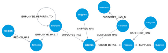
Figure 2.
The general model of the Northwind graph is heterogeneous, directed, and with attributes. It consists of ten types of nodes and ten types of relationships. These nodes represent different entities within the graph, while the relationships denote their connections and interactions. This comprehensive model provides a structured representation of the Northwind dataset, enabling practical analysis and exploration of its interconnected elements.
Given our pursuit of product recommendations, community algorithms could be applied to the graph to recommend products from the same community (3.1). However, due to the specific decision questions guiding the case, path-finding algorithms (task 3.5) are unnecessary, as we are not seeking the shortest, most economical path traversing the entire graph. Similarly, centrality algorithms (task 3.2) are not applicable, since we are not in search of the most influential nodes. While a similarity algorithm (task 3.4) could be employed to identify patterns between products on invoices, we opt not to pursue this path. We focus solely on applying community algorithms (task 3.3) to address the questions. Upon completing stage 3, we verify the adequacy of the information and proceed to stage 4.
In stage 4, to address the questions, we generate a subgraph that includes the orders, products, categories nodes, and the relationships connecting them (task 4.4). To facilitate the recommendation of substitute products (question four), we introduce two new relationships: “buy products” and “buy categories”. We also added a new attribute, “Louvain”, to the products node, resulting from applying graph mining community algorithms (tasks 3.1 and 3.3). This new attribute enables us to recommend substitute products within the same group (tasks 4.1 and 4.2). We then apply summarization based on the new attribute “Louvain”, generating a subgraph (task 4.3). Figure 3 illustrates the subgraph, which initially contains 77 products. The graph is summarised into four groups: the first cluster includes 9 products, the second cluster has 24 products, the third cluster has 20 products, and the last cluster consists of 24 products. Upon completing stage 4, we verify the adequacy of the information and proceed to stage 5.
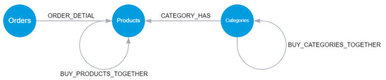
Figure 3.
The view shows the subgraph of orders, products, and categories, revealing the newly established relationships of “buy products together” and “buy categories together”. This condensed representation provides a comprehensive overview of the connections within the dataset, highlighting the associations between purchased products and the co-occurrence of categories in customer orders.
In stage 5, to answer questions 1 and 2, we execute two queries in the Cypher language over the subgraph. Because we want to represent the spatial distribution of nodes and relationships, we use a force-based layout. However, there are other algorithms, e.g., hierarchical. Figure 4 displays the subgraph of orders, products, and categories. In this view, we apply a force-based layout (task 5.1). In addition, we require another visualization to know how many products belong to each category and how many orders each product had. That would allow us to select one or more products, have the data dynamically updated, and do the same with categories or orders. By examining Figure 5, we can observe that when selecting the top 5 best-selling categories together, 59 products and 786 orders have been sold. By performing a drill-down, focusing on category number 4, we discovered 10 products sold and 304 associated orders (task 5.2). Furthermore, we want to apply a rule to display only the subgraph containing the top 5 best-selling products. If we take Figure 4 as a base and apply the rule, we can see the result in Figure 6 (task 5.3), which illustrates the resulting graph featuring 7 products (due to some combinations being repeated), 240 orders, and 3 categories. In addressing the questions, we found no necessity to emphasize structural patterns and attributes (5.4) or to establish a timeline that provides information on forward or backward changes (5.5); hence, these components are not included. Finally, we opted to utilize a dashboard for presenting the results, as depicted in Figure 7. This dashboard incorporates two tables: the first showcases the top five best-selling product category pairs, and the second displays the five best-selling individual product pairs. Additionally, it features a dynamic element—a combo box—allowing users to select a specific product. Upon selection, the dashboard dynamically updates to present both recommended products and alternative options associated with the chosen product. Upon completing stage 5, we verify the adequacy of the information and proceed to stage 6.
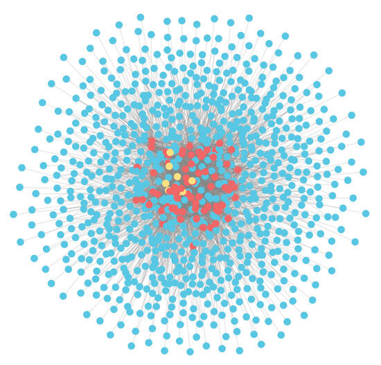
Figure 4.
The subgraph consists of 830 orders (represented in blue), 77 products (represented in red), and 8 categories (represented in yellow), each with new relationships indicating products bought together and categories bought together.
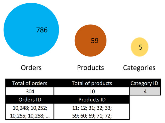
Figure 5.
The top 5 selling categories have been identified and chosen inside the circles. If we exclusively opt for the category with an identifier equal to four, it displays the comprehensive details, including the total number of products, the identifier for each product, the total count of orders, and the identifier for each order.
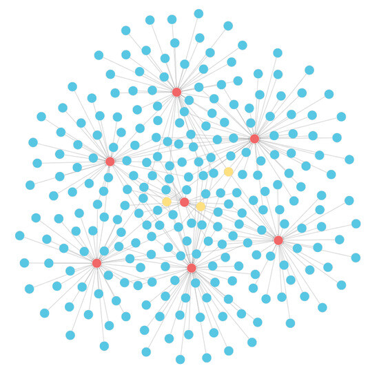
Figure 6.
This subgraph consists of the 7 top-selling items, represented by red nodes, along with the 242 orders in which they appear, denoted by blue nodes. Additionally, the subgraph highlights the three categories to which these items belong, distinguished by yellow nodes. This visual representation clearly explains the relationships between the best-selling items, their order frequencies, and their corresponding categories. By examining this subgraph, valuable insights can be gained regarding the popularity and classification of these items within the dataset.
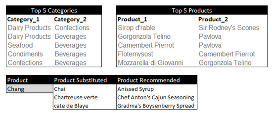
Figure 7.
The dashboard provides an overview of the results addressing the questions. It includes the following information: Top 5 categories; Top 5 products; Product substitutes; Recommended products. By analyzing these insights, users can quickly identify the most popular categories and products, explore alternative options, and receive personalized recommendations based on their preferences. This dashboard serves as a valuable tool for decision making, enabling users to make informed choices and optimize their product selection process.
In Stage 6, completion of all tasks is mandatory. The questions outlined in Stage 1 are the foundation for evaluating the results. The questions of this case were as follows: (1) What are the top 5 categories of products frequently purchased together? (2) Which products are among the top 5 most commonly purchased together? (3) Given a specific product, what are the provided purchase recommendations? (4) Should a product be unavailable, what is the suggested substitute for a recommendation? Based on the analysis, the top 5 categories frequently bought together are Dairy Products and Confections, Dairy Products and Beverages, Seafood and Beverages, Condiments and Beverages, and Confections and Beverages. The top five products often bought together are Sirop d’rable and Sir Rodney’s Scones, Gorgonzola Telino and Pavlova, Camembert Pierrot and Pavlova, Flotemysost and Camembert Pierrot, and Mozzarella di Giovanni and Gorgonzola Telino. If we select Chang as a specific product, the recommended products to purchase together are Aniseed Syrup, Chef Anton’s Cajun Seasoning, Grandma’s Boysenberry Spread, Uncle Bob’s Organic Dried Pears, or Northwoods Cranberry Sauce. If we consider Mozzarella di Giovanni, the substitute products could be Camembert Pierrot, Flotemysost, Geitost, Gorgonzola Telino, Gudbrandsdalsost, Mascarpone Fabioli, Queso Cabrales, Queso Manchego La Pastora, or Raclette Courdavault. The dashboard (Figure 7) can be utilized to select any other product and obtain recommendations or substitute products (task 6.1).
If the information is updated, the recommended categories and products may vary based on customer orders. Since the analysis was performed using data extracted from a relational database within a specific timeframe, it is crucial to document the results associated with a given date. By documenting this information, we can conduct an analysis based on the timeline of product and product category behaviors (task 6.2). The following steps would be to create new questions based on the results (task 6.3).
Because we follow the methodology, we have identified the key categories and products frequently bought together. Additionally, we have developed a dashboard that integrates the results and enables users to select specific products for purchase recommendations or substitute product suggestions.
This approach significantly benefits understanding consumer behavior and enhancing the shopping experience. Businesses can gain valuable insights to optimize their product offerings, conduct targeted marketing campaigns, and improve customer satisfaction by analyzing data based on orders and the interconnections between products and categories.
It is important to note that this case study is based on data extraction from a relational database within a specific period. Therefore, documenting the results associated with a given date and conducting further analysis based on the evolution of orders and product categories is crucial. Updating the information is also essential, as the recommended products and categories may vary based on customer orders.
In summary, the application of the proposed methodology has proven to be effective in the field of product purchase recommendation. This methodology can be adapted to different contexts and databases, providing businesses with a powerful tool to understand and enhance their customers’ purchasing process.
5.2. Airports
Airports are a critical component of global connectivity, and identifying the most important airports within their network of connections is crucial. This case study aims to determine these key airports and recommend investment in their improvement or expansion. Initially, the information is stored in two comma-separated files. We follow the KDG methodology to analyze. Specifically, we use tasks 1.5, 2.1, 2.2, 2.3, 2.4, 3.1, 3.2, 4.1, 4.2, 4.4, 5.6, 6.1, 6.2, and 6.3.
According to the methodology, we should check all tasks of stage 1. However, as in case 1, there are no defined business goals, information requirements, metrics, or project plans. Although tasks 1.1 to 1.4 are missing, the methodology indicates that we must apply at least task 1.5, in which we must define at least one question for decision making that guides the analysis to meet the initial request. In this scenario, we formulate the following decision-making question: What are the most important airports in our network of connections? To refine our response, we establish three subquestions: (1) Which five airports have the highest number of immediate connections with other airports? (2) Which five airports could play a pivotal role in maintaining subsequent connections due to their extensive network ties? (3) What are the top five airports ideally suited for stopovers? (task 1.5).
Following the methodology, we advance to stage 2, where completing all tasks is obligatory. The primary task (2.1) entails conducting an exploratory information analysis. The initial CSV file contains airport details such as name, country, latitude, longitude, and a unique identifier, while the second file provides information on airport connections. Notably, all connections are bidirectional, representing both departure and arrival routes. The files include 225 countries with at least one registered airport. In order to model the graph, we will represent each airport as a node connected to itself using the “Connected-to” relationship, as illustrated in Figure 8 (task 2.2). Progressing to task (2.3), we opt for NEO4J as the data storage solution because it is a graph-based database. Subsequently, we craft a Cypher script to extract information from the CSV files, transforming airport details into nodes with attributes and connections into edges. Lastly, we populate a new database instance with the processed data (task 2.4). With the completion of all tasks in stage 2, we verify the sufficiency of the information and progress to stage 3.
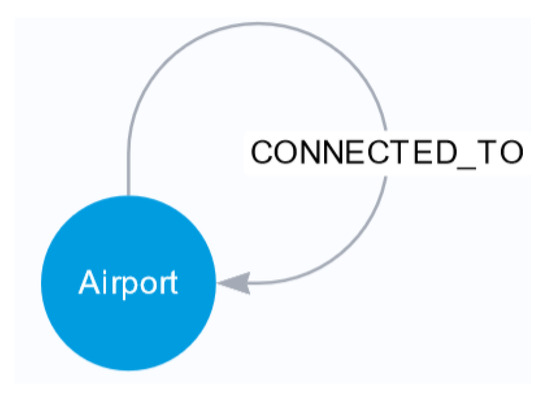
Figure 8.
The general model of the airport graph is homogeneous, directed, and includes attributes. The nodes in the graph represent airports, while the relationships between nodes are of the connected-with type, indicating the connectivity between airports.
In Stage 3, we decided to utilize centrality algorithms for addressing the subquestions related to airports with the most immediate connections, those crucial for continuity, and the ideal stopover airports (task 3.1). Centrality algorithms prove valuable in identifying critical nodes within the network, making them well-suited for our objectives at this stage. We specifically apply them to airport nodes (task 3.2), excluding the application of community, similarity, or pathfinding algorithms (tasks 3.2 to 3.4). Following the completion of Stage 3, we assess the sufficiency of the information before advancing to Stage 4.
In Stage 4, there is no requirement to generate a subgraph for addressing the questions, as we exclusively have nodes of type airports and edges of type connected to, as shown in Figure 8 (task 4.4). We modify the topology and include the attributes of degree, betweenness centrality, and closeness centrality which will be added to the airport nodes. The degree attribute will help answer subquestion 1, while betweenness centrality will provide insights for subquestion 2. The closeness centrality attribute will address subquestion 3 (tasks 4.1 and 4.2). Ultimately, upon applying summarization to both nodes and edges, the outcome is illustrated in Figure 8. Upon completing Stage 4, we verify the adequacy of the information and proceed to stage 5.
In Stage 5, our focus shifts to implementing a dashboard (task 5.6), drawing insights from the tasks accomplished in Stage 4. This dashboard is designed to incorporate three tables. The initial table will present the names of airports and their respective countries, prioritizing the top 5 based on degree centrality. Similarly, the second table will feature the same information, arranged according to betweenness centrality, while the third table will be structured based on closeness centrality (Figure 9). In addition, a secondary dashboard will be accessible. Positioned on the left side of this dashboard is a bar graph featuring the top 5 countries with the highest number of registered airports. Upon selecting one of the countries on the right, the screen dynamically updates, showcasing the top 5 airports based on degree centrality, betweenness centrality, and closeness centrality (refer to Figure 10). Following the conclusion of Stage 5, a thorough verification of the information’s adequacy precedes our progression to Stage 6.
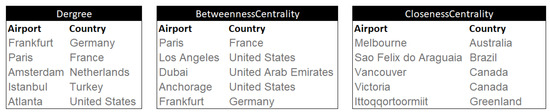
Figure 9.
The dashboard presents the following information: The top 5 airports with the most immediate connections and their corresponding countries. The top 5 critical airports for maintaining continuity, including their respective countries. The top 5 airports are recommended for layovers and their associated countries.
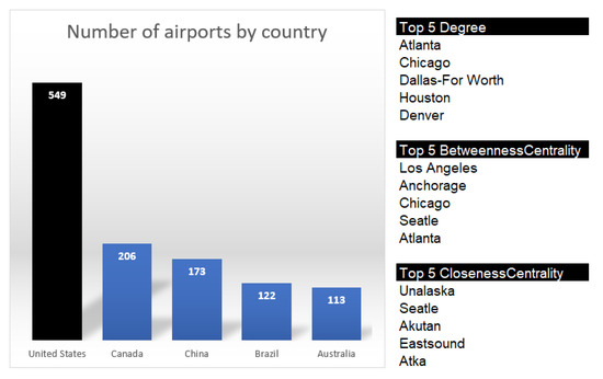
Figure 10.
The dashboard provides the following information: The top 5 countries with the most airports. The top 5 immediate connections, exclusively within the United States. The top 5 critical airports for ensuring continuity in the USA. The top 5 airports recommended for layovers in the USA.
In Stage 6, completion of all tasks is mandatory. Our initial question was: What are the most important airports in our network of connections? To narrow down the answer, we define three subquestions. (1) What five airports have the most immediate connections with other airports? The chosen ones are Frankfurt, Paris, Amsterdam, Istanbul, and Atlanta. (2) What five airports could be vital to giving continuity to the following connections due to their connections with the others? Paris, Los Angeles, Dubai, Anchorage, and Frankfurt score best. (3) What are the five ideal airports for stopovers? Melbourne, Sao Felix do Araguaia, Victoria, Vancouver, and Ittoqqortoormiit are the highest. If we share the data, the airports that appear in more than one category are Frankfurt and Paris (task 6.1).
Based on the results of Figure 9, we can see that the 17 most important airports in the connection network are Frankfurt, Paris, Amsterdam, Istanbul, Atlanta, Los Angeles, Dubai, Anchorage, Melbourne, Sao Felix do Araguaia, Victoria, Vancouver, Ittoqqortoormiit, Neerlerit Inaat, Windhoek, Noumea, and Unalaska. According to the centrality analysis, they are the ones that should be taken into account when investing or expanding.
Finally, we can replicate this analysis in any country. If we take the United States as an example, which has the most significant number of registered airports, we can see in Figure 10 that the airports of Atlanta and Chicago stand out for having the most significant number of immediate connections, but they also appear among the airports with the highest flow. Of note, Seattle appears in two categories (task 6.1). If the information undergoes updates, the outcomes may vary. Considering that the analysis was conducted using data extracted from a flat file within a specific timeframe, it is imperative to document the results tied to a particular date. This documentation enables us to carry out an analysis aligned with the timeline of airports (task 6.2). Furthermore, future endeavors could consider incorporating data on passenger traffic at each airport to enrich the analysis further and explore alternative datasets within the methodology (task 6.3).
In conclusion, analyzing the airport dataset using the proposed methodology yields valuable insights into the network’s structure and successfully identifies the most significant airports. By investing in improving and expanding these airports, we can enhance global connectivity, optimize travel routes, and stimulate economic growth.
5.3. Path Recommendation
In this case, our goal is to establish a series of routes that connect all pre-registered tourist attractions, with a specific emphasis on minimizing the overall cost rather than prioritizing the orientation of the routes. Initially, the data for analysis are sourced from OSM [65], specifically from a quadrant (Figure 11) within Guadalajara, Jalisco, Mexico. We follow the KDG methodology. Specifically, we use tasks 1.5, 2.1, 2.2, 2.3, 2.4, 3.1, 3.5, 4.1, 4.2, 4.4, 5.6, 6.1, 6.2, and 6.3.
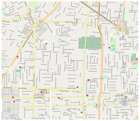
Figure 11.
The provided image depicts the quadrant associated with Guadalajara, Jalisco, Mexico, encompassing the georeferenced information from OpenStreetMaps.
According to the methodology, we should check all tasks of stage 1. However, as in case 1, there are no defined business goals, information requirements, metrics, or project plans. Although tasks 1.1 to 1.4 are missing, the methodology indicates that we must apply at least task 1.5, in which we must define at least one question for decision making that guides the analysis to meet the initial request. In this scenario, we formulate the following decision-making question: Will at least one route allow us to visit all the tourist attractions? (task 1.5).
Following the methodology, we advance to stage 2, where completing all tasks is mandatory. The first task (2.1) entails conducting an exploratory information analysis. The data for analysis are sourced from OSM [65], specifically from a quadrant (Figure 11) within Guadalajara, Jalisco, Mexico. Our analysis centers around the georeferenced information of a quadrant in Guadalajara, Jalisco, Mexico. Specifically, we aim to identify the paths linking the museums within this quadrant. We utilize OpenStreetMaps (OSM) to obtain the necessary data, which provides valuable geospatial information (taks 2.1). Progressing to task 2.2, our graph model consists of two types of nodes: user and point. Since OSM is a community-driven platform, it tracks the users who edit each point or set of points on the map. Additionally, the points on the map are identified by a unique identifier, latitude, and longitude coordinates. Some points may also have additional attributes, such as the brand name for businesses such as Oxxo or 7-Eleven, contact telephone numbers, street names, detailed descriptions, or indicators of being a tourist attraction. Although points have no inherent connection, we will establish relationships and incorporate distance information. The graph model is illustrated in Figure 12. Continue with task 2.3. We chose NEO4J as the data storage solution because it is a graph-based database. Subsequently, we extract the latitude and longitude coordinates of the sites classified by OSM as tourist attractions.
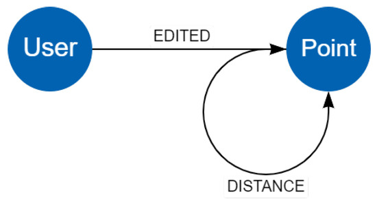
Figure 12.
The general attractions graph model consists of a homogeneous and directed graph with attributes. It includes two types of nodes and two types of relationships.
Furthermore, we transform the OSM information into a graph-based database. Firstly, we export the data from the selected quadrant in Guadalajara as an XML file. Secondly, we develop a script utilizing the cypher language to convert each point into a node, extract their attributes, and insert the information into NEO4J. Each node includes essential details such as a unique identifier, latitude, and longitude. Thirdly, we calculate the geodesic distance between every pair of nodes and establish a relationship called “distance” with the corresponding attribute “geodesicDist”, containing the calculated value. These data are then incorporated into the graph database (task 2.4). Having completed all tasks in stage 2, we verified the sufficiency of the information and progressed to stage 3.
In Stage 3, the decision was made to employ path-finding algorithms to address the route that enables us to visit all the museums (task 3.1). Path-finding algorithms are particularly advantageous when the goal is to identify optimal routes, determine the shortest paths, or analyze flow patterns within the network. Consequently, centrality, community, or similarity algorithms are not applied in this context. Instead, the Minimum Spanning Tree algorithm (MST) is implemented to identify the path with the least total weight, facilitating the visitation of all museums (task 3.5). After the completion of Stage 3, a thorough evaluation of information adequacy precedes our progression to Stage 4.
In Stage 4, we generate a subgraph to identify the points with the tourism attribute, whose value corresponds to a museum. The outcome yields 11 nodes and 121 relationships (Figure 13) (task 4.4). To determine the shortest path connecting all the museums, we modify the graph’s topology by introducing relationships with the lowest weights among the museums (task 4.1). Additionally, we incorporate a relationship named MST resulting from applying the minimum spanning tree algorithm to identify the path with the least total weight that allows us to visit all the museums. These modifications in topology and the inclusion of a new structural attribute led to the creation of the subgraph depicted in Figure 13 (task 4.2). Upon completing Stage 4, we verify the adequacy of the information and proceed to stage 5.
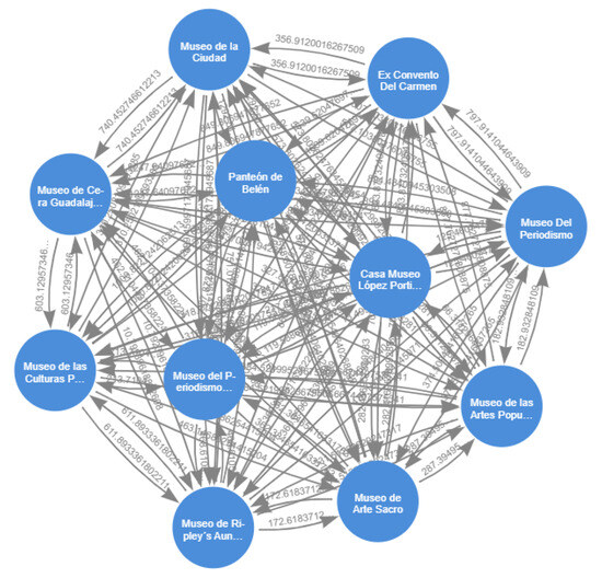
Figure 13.
The subgraph comprises points registered in the graph database, specifically representing museums and their corresponding georeferenced distances.
In Stage 5, we emphasize implementing a dashboard (Figure 14) to showcase the eleven museums and the Minimum Spanning Tree, enabling visitation to each (task 5.6). Upon the completion of Stage 5, a comprehensive verification of the information’s adequacy precedes our transition to Stage 6.
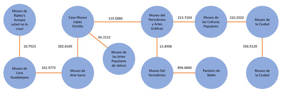
Figure 14.
This subgraph incorporates the eleven museums and the minimum spanning tree that allows for visiting all of them.
In Stage 6, completion of all tasks is mandatory. The initial question was looking for a network of connections among pre-registered tourist attractions to minimize the total cost while disregarding the direction of the connections. We achieved this goal by obtaining the minimum spanning tree that allows us to visit the following eleven museums: Museo de Ripley’s Aunque usted no lo crea!, Panteón de Belén, Museo Del Periodismo, Museo del Periodismo y Artes Gráficas, Museo de la Ciudad, Museo de las Culturas Populares, Museo de Cera Guadalajara, Museo de Arte Sacro, Casa Museo López Portillo, Ex Convento Del Carmen, and Museo de las Artes Populares de Jalisco. Thus, we fulfilled the requirement and answered the question (task 6.1).
Given the dynamic nature of OSM, it is crucial to accurately document the findings with a specific date, considering the continuous addition of new tourist attractions. Since the analysis was based on an OSM extract from a specific period, it is essential to ensure that the results are associated with the corresponding date. By continuously monitoring and analyzing the behavior of the information, we can adapt and optimize the path recommendation system to accommodate future updates (task 6.2). In the following steps, we could expand the quadrant of the map or choose another city (task 6.3).
In conclusion, implementing the proposed methodology has yielded significant results in establishing a network of connections among pre-registered tourist attractions, resulting in minimized costs when visiting the eleven museums. The analysis performed on the OSM extract has provided valuable insights into the connectivity patterns of these attractions. The use of this methodology in the tourism domain shows its potential to enhance the visitor experience and optimize travel routes in various regions.
6. Discussion
The paper aims to address critical aspects of knowledge discovery in graph databases comprehensively. Firstly, it identifies transformation and exploration activities that leverage existing knowledge of data relationships. Despite their significance in graph theory, current methodologies have inadequately addressed these activities. Moreover, the paper acknowledges the limitations of well-known methodologies such as CRISP-DM when applied to graph analytics, as it is focused on tabular data and the guidelines provided by these methodologies are very general; moreover, it does not take into account the challenges addressed when it is required to model data as a graph. Therefore, there is a gap in those methodologies between the type of information, the tasks, the visualization used, and what is required for graph-based analysis.
In order to address these limitations, the paper introduces KDG a novel methodology specifically tailored for knowledge discovery in graph databases. This methodology offers a systematic approach to uncovering valuable insights from graph-structured data, empowering researchers and practitioners to extract meaningful patterns and relationships effectively.
To showcase the methodology, we presented three case studies that show its application to address various business problems. These examples describe how the methodology can competently address various challenges, underscoring its versatility and practicality.
KDG methodology can be compared with others in terms of the tasks we described in Section 4. We have selected the three most representative methodologies in the literature for knowledge discovery. We present in Table 1 a mapping of each task with the steps of CRISP-DM [7], DST [14], and KDD [6]; each row shows the relationship among one KDG’s task and a step or steps in other methodologies. However, in each stage of our methodology, there is no one-to-one correspondence between our tasks and the steps described in other methodologies. This is because the methodologies were not developed to work specifically with information represented as a graph. Furthermore, the steps of these methodologies associated with task 3.1 (Select graph mining algorithms) are related to data mining algorithms in general, not useful for graph mining.

Table 1.
Mapping the KDG’s tasks to CRISP-DM, DST, and KDD steps.
In summary, the paper makes significant contributions to knowledge discovery in graph databases by identifying transformation and exploration activities, addressing the limitations of existing methodologies, introducing a novel methodology, and providing concrete examples of its real-world application in business scenarios. The methodology is well-suited for analyzing highly interconnected information. However, if the analysis involves other types of information, this methodology may not be the most suitable choice. The user should understand the capabilities inherent in working with graphs. While the user will be provided with a guide to conduct the analysis, foundational knowledge of techniques, such as graph mining algorithms, is essential. The user must not be an expert but familiar with the subject. As part of our future work, we plan to integrate Machine Learning Operations (MLOps) and DevOps practices into our methodology to enhance its effectiveness and efficiency. By incorporating MLOps principles, we aim to streamline machine learning models’ development, deployment, and management, ensuring smooth and scalable operations. Furthermore, we intend to validate the robustness of our methodology by applying it to a broader range of case studies, enabling us to gather more insights and validate them in different business scenarios.
Author Contributions
Conceptualization, V.H.O.-G., L.G.-P., F.C. and M.A.-M.; Methodology, V.H.O.-G., L.G.-P. and F.C.; Software, V.H.O.-G.; Validation, V.H.O.-G., L.G.-P., F.C. and M.A.-M.; Formal analysis, L.G.-P.; Investigation, L.G.-P. and F.C.; Data curation, V.H.O.-G.; Writing—original draft, V.H.O.-G.; Writing—review & editing, V.H.O.-G., L.G.-P., F.C. and M.A.-M.; Visualization, V.H.O.-G. and M.A.-M.; Supervision, L.G.-P. and F.C. All authors have read and agreed to the published version of the manuscript.
Funding
This research received no external funding.
Institutional Review Board Statement
Not applicable.
Informed Consent Statement
Not applicable.
Data Availability Statement
The data presented in this study are available on request from the author (vortega@iteso.mx).
Conflicts of Interest
The authors declare no conflict of interest.
Abbreviations
The following abbreviations are used in this manuscript:
| SQL | Structured Query Language |
| NOSQL | Not Only Structured Query Language |
| CRISP-DM | Cross-Industry Standard Process for Data Mining |
| BIM | Business Intelligence Model |
| MLOps | Machine Learning Operations |
| OSM | Open Street Maps |
| CSV | Comma Separated Values |
| GDB | Graph Database |
| RDB | Relational Database |
| SMART | Specific, Measurable, Achievable, Relevant, and Time-bound |
| KDD | Knowledge Discovery in Databases |
| SEMMA | Sample, Explore, Modify, Model, and Assess |
| DST | Decision Support Tool |
| EDA | Exploratory Data Analysis |
| PDA | Predictive Data Analysis |
| ASUM | Analytics Solutions Unified Method |
| CASP-DM | Context-Aware Standard Process for Data Mining |
| FMDS | Foundational Methodology for Data Science |
| TDSP | Team Data Science Process |
| DST | Data Science Trayectory |
| KDG | Knowledge Discovery in Graphs |
References
- Fernandes, D.; Bernardino, J. Graph Databases Comparison: AllegroGraph, ArangoDB, InfiniteGraph, Neo4J, and OrientDB. In Proceedings of the 7th International Conference on Data Science, Technology and Applications (DATA 2018), Volterra, Italy, 13–16 September 2018; pp. 373–380. [Google Scholar]
- Lysenko, A.; Roznovăţ, I.A.; Saqi, M.; Mazein, A.; Rawlings, C.J.; Auffray, C. Representing and querying disease networks using graph databases. BioData Min. 2016, 9, 1–19. [Google Scholar] [CrossRef]
- Doğan, B. The Importance of Graph Databases in Detection of Organized Financial Crimes. In The Impact of Artificial Intelligence on Governance, Economics and Finance; Springer: Berlin/Heidelberg, Germany, 2022; Volume 2, pp. 147–155. [Google Scholar]
- Czerepicki, A. Application of graph databases for transport purposes. Bull. Pol. Acad. Sci. Tech. Sci. 2016, 64, 457–466. [Google Scholar] [CrossRef][Green Version]
- Sayeb, Y.; Jebri, M.; Ghezala, H.B. A graph based recommender system for managing COVID-19 Crisis. Procedia Comput. Sci. 2022, 196, 348–355. [Google Scholar] [CrossRef] [PubMed]
- Fayyad, U.M.; Piatetsky-Shapiro, G.; Smyth, P. Knowledge Discovery and Data Mining: Towards a Unifying Framework. Proceedings of Second International Conference on Knowledge Discovery and Data Mining (KDD-96), Portland, OR, USA, 2–4 August 1996; Volume 96, pp. 82–88. [Google Scholar]
- Wirth, R.; Hipp, J. CRISP-DM: Towards a standard process model for data mining. In Proceedings of the 4th International Conference on the Practical Applications of Knowledge Discovery and Data Mining, Manchester, UK, 11–13 April 2000; Volume 1, pp. 29–39. [Google Scholar]
- Sarma, K.S. Predictive Modeling with SAS Enterprise Miner: Practical Solutions for Business Applications; SAS Institute: Cary, NC, USA, 2017. [Google Scholar]
- Chakrabarti, D. Graph Mining. In Encyclopedia of Machine Learning; Sammut, C., Webb, G.I., Eds.; Springer: Boston, MA, USA, 2010; pp. 469–471. [Google Scholar] [CrossRef]
- IBM Analytics Solutions Unified Method (ASUM). Available online: http://gforge.icesi.edu.co/ASUM-DM_External/index.htm#cognos.external.asum-DM_Teaser/deliveryprocesses/ASUM-DM_8A5C87D5.html_desc.html?proc=_0eKIHlt6EeW_y7k3h2HTng&path=_0eKIHlt6EeW_y7k3h2HTng (accessed on 14 September 2023).
- Martínez-Plumed, F.; Ochando, L.C.; Ferri, C.; Flach, P.A.; Hernández-Orallo, J.; Kull, M.; Lachiche, N.; Ramírez-Quintana, M.J. CASP-DM: Context Aware Standard Process for Data Mining. CoRR 2017, arXiv:1709.09003. [Google Scholar]
- Foundational Methodology for Data Science. Available online: https://www.ibm.com/downloads/cas/WKK9DX51 (accessed on 14 September 2023).
- Team Data Science Process. Available online: https://docs.microsoft.com/en-us/azure/machine-learning/team-data-science-process (accessed on 14 September 2023).
- Martínez-Plumed, F.; Contreras-Ochando, L.; Ferri, C.; Hernández-Orallo, J.; Kull, M.; Lachiche, N.; Ramirez-Quintana, M.J.; Flach, P. CRISP-DM twenty years later: From data mining processes to data science trajectories. IEEE Trans. Knowl. Data Eng. 2019, 33, 3048–3061. [Google Scholar] [CrossRef]
- Studer, S.; Bui, T.B.; Drescher, C.; Hanuschkin, A.; Winkler, L.; Peters, S.; Müller, K.R. Towards CRISP-ML (Q): A machine learning process model with quality assurance methodology. Mach. Learn. Knowl. Extr. 2021, 3, 392–413. [Google Scholar] [CrossRef]
- Horkoff, J.; Barone, D.; Jiang, L.; Yu, E.; Amyot, D.; Borgida, A.; Mylopoulos, J. Strategic business modeling: Representation and reasoning. Softw. Syst. Model. 2014, 13, 1015–1041. [Google Scholar] [CrossRef]
- Kumar, D.; Showrov, M.I.H. A data mining framework for social graph generation and analysis. In Proceedings of the 2nd International Conference on Innovation in Engineering and Technology (ICIET), Harbin, China, 20–22 January 2019; pp. 1–6. [Google Scholar]
- Pienta, R.; Hohman, F.; Endert, A.; Tamersoy, A.; Roundy, K.; Gates, C.; Navathe, S.; Chau, D.H. VIGOR: Interactive visual exploration of graph query results. IEEE Trans. Vis. Comput. Graph. 2017, 24, 215–225. [Google Scholar] [CrossRef] [PubMed]
- Bok, K.; Yoo, S.; Choi, D.; Lim, J.; Yoo, J. In-Memory Caching for Enhancing Subgraph Accessibility. Appl. Sci. 2020, 10, 5507. [Google Scholar] [CrossRef]
- Chen, C.; Yan, X.; Zhu, F.; Han, J.; Philip, S.Y. Graph OLAP: A multi-dimensional framework for graph data analysis. Knowl. Inf. Syst. 2009, 21, 41–63. [Google Scholar] [CrossRef]
- Mcgee, F.; Ghoniem, M.; Melançon, G.; Otjacques, B.; Pinaud, B. The state of the art in multilayer network visualization. In Computer Graphics Forum; Wiley Online Library: Hoboken, NJ, USA, 2019; Volume 38, pp. 125–149. [Google Scholar]
- Nararatwong, R.; Kertkeidkachorn, N.; Ichise, R. Knowledge graph visualization: Challenges, framework, and implementation. In Proceedings of the IEEE 3rd International Conference on Artificial Intelligence and Knowledge Engineering (AIKE), Laguna Hills, CA, USA, 9–11 December 2020; pp. 174–178. [Google Scholar]
- Shchur, O.; Mumme, M.; Bojchevski, A.; Günnemann, S. Pitfalls of graph neural network evaluation. arXiv 2018, arXiv:1811.05868. [Google Scholar]
- Alshahrani, M.; Thafar, M.A.; Essack, M. Application and evaluation of knowledge graph embeddings in biomedical data. PeerJ Comput. Sci. 2021, 7, e341. [Google Scholar] [PubMed]
- Shrivastava, S.; Pal, S.N. Graph mining framework for finding and visualizing substructures using graph database. In Proceedings of the International Conference on Advances in Social Network Analysis and Mining, Athens, Greece, 20–22 July 2009; pp. 379–380. [Google Scholar]
- Nasiri, A.; Nalchigar, S.; Yu, E.; Ahmed, W.; Wrembel, R.; Zimanyi, E. From indicators to predictive analytics: A conceptual modelling framework. In Proceedings of the IFIP Working Conference on The Practice of Enterprise Modeling, Leuven, Belgium, 22–24 November 2017; pp. 171–186. [Google Scholar]
- Yu, E. Modeling Strategic Relationships for Process Reengineering. Soc. Model. Requir. Eng. 2011, 11, 66–87. [Google Scholar]
- Schroeder, D.T.; Pogorelov, K.; Langguth, J. Fact: A framework for analysis and capture of twitter graphs. In Proceedings of the 2019 Sixth International Conference on Social Networks Analysis, Management and Security (SNAMS), Granada, Spain, 22–25 October 2019; pp. 134–141. [Google Scholar]
- Qiao, F.; Zhang, X.; Li, P.; Ding, Z.; Jia, S.; Wang, H. A parallel approach for frequent subgraph mining in a single large graph using spark. Appl. Sci. 2018, 8, 230. [Google Scholar] [CrossRef]
- Zhang, J.; Li, T.; Jiang, Z.; Hu, X.; Jazayeri, A. A Noval Weighted Meta Graph Method for Classification in Heterogeneous Information Networks. Appl. Sci. 2020, 10, 1603. [Google Scholar] [CrossRef]
- Lee, K.; Jung, H.; Hong, J.S.; Kim, W. Learning Knowledge Using Frequent Subgraph Mining from Ontology Graph Data. Appl. Sci. 2021, 11, 932. [Google Scholar] [CrossRef]
- Dunne, C.; Shneiderman, B. Motif simplification: Improving network visualization readability with fan, connector, and clique glyphs. In Proceedings of the SIGCHI Conference on Human Factors in Computing Systems, Paris, France, 27 April–2 May 2013; pp. 3247–3256. [Google Scholar]
- West, D.B. Introduction to Graph Theory; Prentice Hall: Upper Saddle River, NJ, USA, 2001; Volume 2. [Google Scholar]
- Robinson, I.; Webber, J.; Eifrem, E. Graph Databases: New Opportunities for Connected Data; O’Reilly Media, Inc.: Sebastopol, CA, USA, 2015. [Google Scholar]
- Les MacLeod EdD. Making SMART goals smarter. Physician Exec. 2012, 38, 68. [Google Scholar]
- ISO/IEC/IEEE 29148:2018(E); ISO/IEC/IEEE International Standard-Systems and Software Engineering–Life Cycle Processes–Requirements Engineering. IEEE: Piscataway, NJ, USA, 2018; pp. 1–104. [CrossRef]
- Lovett, J. Social Media Metrics Secrets; John Wiley & Sons: Hoboken, NJ, USA, 2011. [Google Scholar]
- Pendleton, M.; Garcia-Lebron, R.; Cho, J.H.; Xu, S. A survey on systems security metrics. ACM Comput. Surv. (CSUR) 2016, 49, 1–35. [Google Scholar] [CrossRef]
- Reich, B.H.; Wee, S.Y. Searching for Knowledge in the PMBOK® Guide. Proj. Manag. J. 2006, 37, 11–26. [Google Scholar] [CrossRef]
- Hammond, J.S.; Keeney, R.L.; Raiffa, H. Smart Choices: A Practical Guide to Making Better Decisions; Harvard Business Review Press: Brighton, MA, USA, 2015. [Google Scholar]
- Bowell, T.; Kemp, G. Critical Thinking: A Concise Guide; Routledge: London, UK, 2014. [Google Scholar]
- Kojima, R.; Legaspi, R.; Wada, S. Trip Destination Prediction by Cross-City Exploratory Data Analysis Approach in People Flow Data. In Proceedings of the IEEE International Conference on Big Data (Big Data), Osaka, Japan, 17–20 December 2022; pp. 6547–6552. [Google Scholar] [CrossRef]
- Fuentes, A. Become a Python Data Analyst: Perform Exploratory Data Analysis and Gain Insight into Scientific Computing Using Python; Packt Publishing Ltd.: Birmingham, UK, 2018. [Google Scholar]
- Uzhga-Rebrov, O.; Grabusts, P. Comparative Evaluation of Four Methods for Exploratory Data Analysis. In Proceedings of the 2021 62nd International Scientific Conference on Information Technology and Management Science of Riga Technical University (ITMS), Riga, Latvia, 14–15 October 2021; pp. 1–5. [Google Scholar] [CrossRef]
- Mostajabi, F.; Safaei, A.A.; Sahafi, A. A Systematic Review of Data Models for the Big Data Problem. IEEE Access 2021, 9, 128889–128904. [Google Scholar] [CrossRef]
- Lal, M. Neo4j Graph Data Modeling; Packt Publishing Ltd.: Birmingham, UK, 2015. [Google Scholar]
- Ortega, V.; Ruiz, L.; Gutierrez, L.; Cervantes, F. A selection process of graph databases based on business requirements. In Proceedings of the International Conference on Software Process Improvement, Leon, Mexico, 23–25 October 2019; pp. 80–90. [Google Scholar]
- Bansal, S.K.; Kagemann, S. Integrating Big Data: A Semantic Extract-Transform-Load Framework. Computer 2015, 48, 42–50. [Google Scholar] [CrossRef]
- Maria Carina, R. Learning Pentaho Data Integration 8 CE-Third Edition: Get Up and Running with the Pentaho Data Integration Tool Using This Hands-On, Easy-to-Read Guide; Packt Publishing: Birmingham, UK, 2017. [Google Scholar]
- Tirthajyoti, S.; Shubhadeep, R. Data Wrangling with Python: Creating Actionable Data From Raw Sources; Packt Publishing: Birmingham, UK, 2019. [Google Scholar]
- Koutra, D.; Faloutsos, C. Individual and Collective Graph Mining: Principles, Algorithms, and Applications; Springer Nature: Berlin/Heidelberg, Germany, 2022. [Google Scholar]
- Needham, M.; Hodler, A.E. Graph Algorithms: Practical Examples in Apache Spark and Neo4j; O’Reilly Media: Sebastopol, CA, USA, 2019. [Google Scholar]
- Chintalapudi, S.R.; Prasad, M.H.M.K. A survey on community detection algorithms in large scale real world networks. In Proceedings of the 2015 2nd International Conference on Computing for Sustainable Global Development (INDIACom), New Delhi, India, 11–13 March 2015; pp. 1323–1327. [Google Scholar]
- Buttler, D. A Short Survey of Document Structure Similarity Algorithms; Technical Report; Lawrence Livermore National Lab. (LLNL): Livermore, CA, USA, 2004. [Google Scholar]
- Lawande, S.R.; Jasmine, G.; Anbarasi, J.; Izhar, L.I. A Systematic Review and Analysis of Intelligence-Based Pathfinding Algorithms in the Field of Video Games. Appl. Sci. 2022, 12, 5499. [Google Scholar] [CrossRef]
- Barabási, A.L. Network science. Philos. Trans. R. Soc. A Math. Phys. Eng. Sci. 2013, 371, 20120375. [Google Scholar] [CrossRef] [PubMed]
- Liu, Y.; Safavi, T.; Dighe, A.; Koutra, D. Graph summarization methods and applications: A survey. ACM Comput. Surv. (CSUR) 2018, 51, 1–34. [Google Scholar] [CrossRef]
- Erciyes, K. Complex Networks: An Algorithmic Perspective; CRC Press: Boca Raton, FL, USA, 2014. [Google Scholar]
- Cherven, K. Mastering Gephi Network Visualization; Packt Publishing Ltd.: Birmingham, UK, 2015. [Google Scholar]
- Ward, M.O.; Grinstein, G.; Keim, D. Interactive Data Visualization: Foundations, Techniques, and Applications; CRC Press: Boca Raton, FL, USA, 2010. [Google Scholar]
- Dileep, S.; Manoj, R.; Adarsh, M.; Harikumar, S. Comparing the Effectiveness of Data Visualization Techniques for Discovering Disease Relationships in a Complex Network Dataset. In Proceedings of the 2023 7th International Conference on Trends in Electronics and Informatics (ICOEI), Tirunelveli, India, 11–13 April 2023; pp. 1486–1492. [Google Scholar] [CrossRef]
- Wajahat, A.; Nazir, A.; Akhtar, F.; Qureshi, S.; Ullah, F.; Razaque, F.; Shakeel, A. Interactively Visualize and Analyze Social Network Gephi. In Proceedings of the 3rd International Conference on Computing, Mathematics and Engineering Technologies (iCoMET), Sukkur, Pakistan, 29–30 January 2020; pp. 1–9. [Google Scholar] [CrossRef]
- Chaudhary, A.; Jain, N.; Kumar, A. Tools for Social Network Analysis and Mining. In Proceedings of the 11th International Conference on System Modeling & Advancement in Research Trends (SMART), Moradabad, India, 16–17 December 2022; pp. 1063–1067. [Google Scholar] [CrossRef]
- Islam, M.; Jin, S. An Overview of Data Visualization. In Proceedings of the International Conference on Information Science and Communications Technologies (ICISCT), Karachi, Pakistan, 9–10 March 2019; pp. 1–7. [Google Scholar] [CrossRef]
- OpenStreetMap. 2023. Available online: https://www.openstreetmap.org (accessed on 14 September 2023).
Disclaimer/Publisher’s Note: The statements, opinions and data contained in all publications are solely those of the individual author(s) and contributor(s) and not of MDPI and/or the editor(s). MDPI and/or the editor(s) disclaim responsibility for any injury to people or property resulting from any ideas, methods, instructions or products referred to in the content. |
© 2024 by the authors. Licensee MDPI, Basel, Switzerland. This article is an open access article distributed under the terms and conditions of the Creative Commons Attribution (CC BY) license (https://creativecommons.org/licenses/by/4.0/).