A Novel Reverse Combination Configuration to Reduce Mismatch Loss for Stratospheric Airship Photovoltaic Arrays

Abstract

Enhancing the output power of stratospheric airship photovoltaic arrays during months with weak irradiance is crucial for extending the endurance of airships. Models for predicting the output power of photovoltaic arrays and the phenomenon of mismatch losses have been proposed. However, static reconstruction schemes to reduce or eliminate mismatch losses have not been studied. In this paper, an output power model for stratospheric airship arrays including the solar radiation and irradiance distribution is established. The characteristics of the irradiance distribution for the photovoltaic array (PV) are investigated through simulation. Furthermore, an innovative reverse combination configuration is developed and compared to the SP and TCT configurations in terms of performance, mismatch loss and fill factor. Finally, simulations are conducted for a full-day irradiance period of 4 days in a real wind field. The simulation results demonstrate that the proposed RC configuration significantly reduces mismatch losses and output power fluctuations, thereby enhancing the PV array’s output power. This research provides interesting insights for the design of PV array topologies for stratospheric airships.

1. Introduction

Stratospheric airships are controllable aerostats that maintain altitude through buoyancy. They reside in the stratosphere at an approximate altitude of 20 km, making them ideal for long-duration missions such as communication relays, stationary observations, and disaster forecasting [1,2]. To accomplish these tasks, a solar-powered renewable energy system is necessary to provide stable power for the propulsion, avionics, and payload systems [3]. The airship’s renewable energy system primarily consists of a photovoltaic (PV) array, a DC/DC converter with maximum power point tracking (MPPT) functionality, and energy storage batteries [4].

The performance of the energy system determines the airship’s cruising capability, with the primary influencing factors being the conversion efficiency of solar cells and the energy density of the storage batteries. Pande [5] analyzed the impact of the solar cell conversion efficiency, areal density, and specific energy of the secondary storage system on the length and total weight of the airship. The research findings indicate that when the wind speed exceeds 14 m/s, the performance of the high energy density triple-junction cells surpasses that of the thin-film battery. Li et al. [6] developed a thermal model for PV arrays to assess the output capacity. Their findings indicate that excessively high operating temperatures can significantly reduce the conversion efficiency of PV arrays. Du [7] introduced the angle loss coefficient to further refine the aforementioned model. The results indicate that, without taking into account the impact of the winter solstice angle loss, the maximum power of the solar panel array during daylight hours is overestimated by 12.3%.

Constrained by the current efficiency of solar cells [8] and the effective capacity of energy storage batteries, a larger-scale energy system is required to meet the high wind resistance demands of airships [9,10], resulting in excessive volume and weight of the airship [11,12]. Researchers aim to improve the power supply capacity of the airship’s energy system by optimizing the utilization of PV arrays and energy management to meet the energy balance requirements.

Enhancement of the PV array’s power supply capacity can be effectively achieved through layout optimization and thermal control. Meng et al. [13] conducted a multi-objective optimization design for the thermal insulation and heat dissipation layers of photovoltaic arrays, resulting in an increase in the power output per unit area from 88.5 W to 95.4 W. Lv et al. [14] proposed a genetic algorithm-based model for optimizing the layout of PV arrays, resulting in the identification of the optimal arrangement for PV arrays under four typical operational conditions. Alam [15] proposed a multidisciplinary optimization method for HAA based on genetic algorithms, achieving an optimal layout of five deployment positions for PV arrays. Jiang et al. [16] analyzed the sensitivity of power output to the rotational angle and installation angle of PV arrays during cruising, and indicated that the optimal installation angle for PV arrays should be controlled within ±20°.

To further enhance the energy acquisition during the operation of airships, an increasing amount of research is focusing on the design of flight strategies and attitude planning. Wang [17] analyzed the sensitivity of the airship’s attitude angles to PV arrays and found that the yaw angle has the greatest impact. Zhu et al. [18] proposed an optimal yaw angle strategy in quasi-zero wind fields, aiming to maximize the output power of the PV array. The result demonstrates that the optimal yaw angle varies with the working dates and latitude and is primarily concentrated at 0° and 180°. Zhang [19] devised an integrated attitude manipulation strategy encompassing roll, pitch, and yaw control, resulting in a substantial enhancement of energy production and wind resistance capabilities of airships. Shan [20] proposed an airship energy management scheme based on a position energy storage strategy. This approach optimized the allocation of energy throughout the day, thereby enhancing the airship’s endurance.

Furthermore, researchers proposed strategies for controlling the angle of irradiation incidence to enhance the PV arrays’ output power. The solar tracking device, capable of adjusting the angle between the irradiation vector and solar cell plane in real time, is regarded as an effective method for improving PV energy collection [21,22]. Lv [23] designed a rotatable PV array system that tracks the sun’s incident angle by rotating around the airship envelope, obtaining a daily energy output increase of over 40%. Du [24] analyzed the differences between the thermal distribution characteristics of the rotatable and the conventional PV array. The result showed that the temperatures of the improved airship are slight higher than those of the traditional airship at 04:00 to 10:00 and 14:00 to 20:00. Zhu [25] devised a comprehensive optimization strategy for the rotation angle and yaw angle in a real wind field.

Existing research extensively discusses approaches to improve energy acquisition in airship energy systems. However, there is limited research on the impact of the PV array topology on its output capacity. Liu et al. [26] conducted a study on the output performance of PV arrays under partially shaded conditions, focusing on four configurations: series–parallel (SP), bridge-link (BL), honeycomb (HC), and total cross-tied (TCT). The results indicated that, in most cases, the TCT configuration exhibited the best performance. However, in high latitude regions during winter and spring seasons, the rate of energy improvement is less than 10%. Under non-uniform irradiation conditions, “mismatch loss” still profoundly affects the output performance of TCT-configured photovoltaic arrays [27,28]. Static reconfiguration is considered an effective method for mitigating mismatch loss by dispersing local shading. Extensive research has been conducted in this field, with numerous studies available, including the Su Do Ku configuration [29], Lo Shu technique [30], odd–even structure [31], and Latin square arrangement [32]. However, there is a significant lack of research specifically focused on airship PV arrays. Therefore, it is necessary to investigate the issue of mismatch losses of airship PV arrays and conduct static reconfiguration optimization. This holds significant value for enhancing the power capacity and stability of the energy system.

The novelty of this paper lies in the proposal of a novel reverse combination (RC) configuration. This configuration effectively addresses the mismatch loss of stratospheric airship PV arrays and enhances the output power, thereby alleviating the energy scarcity issue. The power output model for stratospheric airship PV arrays is established. The characteristics of the irradiance distribution for typical operating conditions are investigated. The principles and static reconfiguration scheme of the reverse combination configuration are introduced. A comparison is made between the proposed configuration and the classic SP and TCT configurations, considering the characteristic curves, mismatch loss power, and fill factor. Finally, a simulation of daily energy generation in a real wind field demonstrates that the RC configuration maintains the highest output power throughout the full irradiance process, effectively mitigating energy shortages during periods of weak irradiance.

2. Modeling

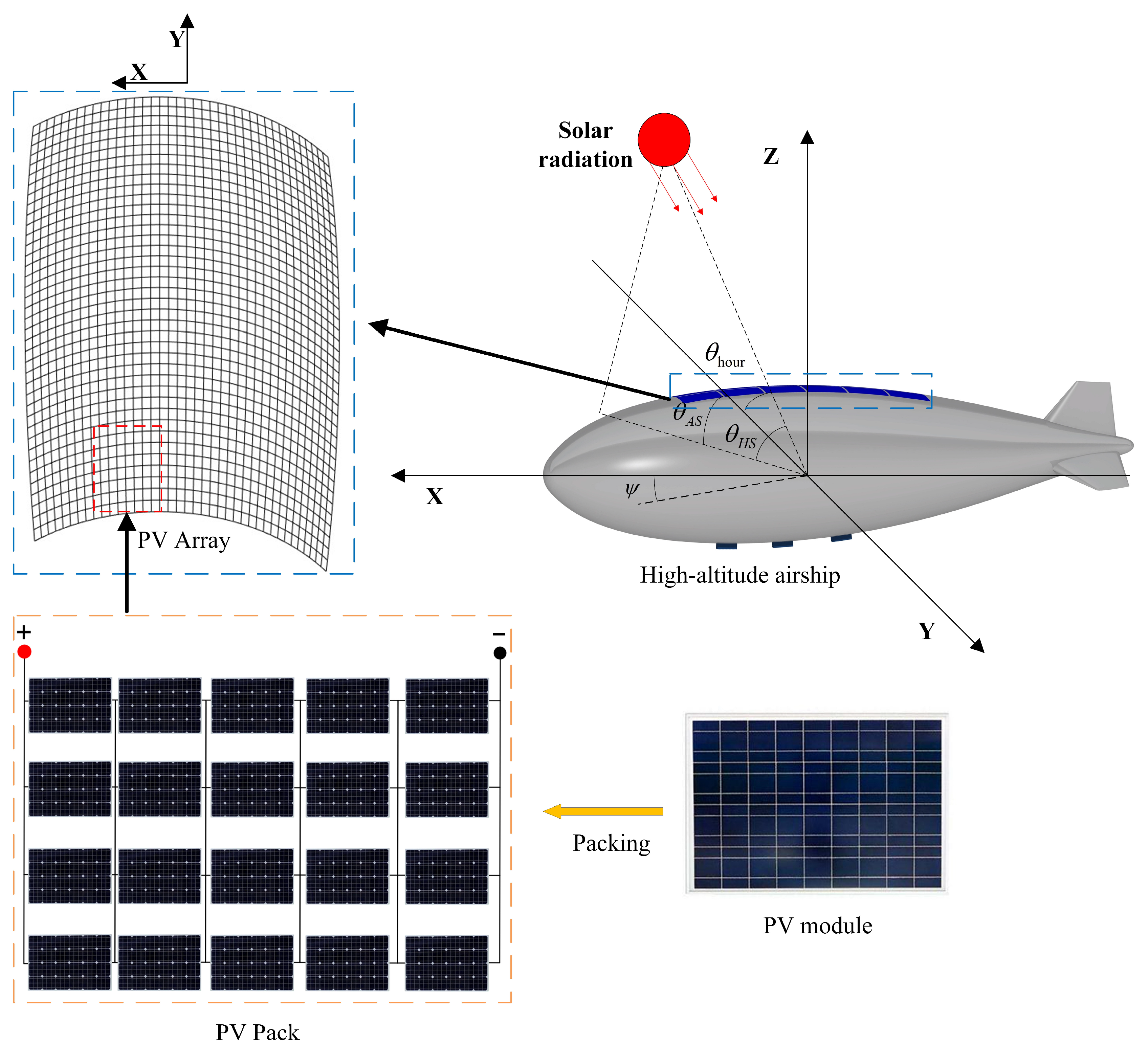
2.1. Solar Radiation Model

The radiation received by the PV arrays primarily consists of direct solar radiation and scattered solar radiation. [33] The direct radiation intensity at the cruising altitude of the airship can be expressed as [34]

$$I_{d0}={\tau }_h\cdot \left(\frac{1+e_e\cdot \cos ({\lambda }_e)}{1-e_e^2}\right)\cdot 1367$$

(1)

where $e_e$ is the orbital eccentricity of Earth, with a value of 0.016708, ${\tau }_h$ is the atmospheric transmissivity, and ${\lambda }_e$ is the true anomaly, which can be given by

$${\lambda }_e={\theta }_{day}+2e_e\cdot \sin ({\theta }_{day})+1.25e_e^2\cdot \sin (2{\theta }_{day})$$

(2)

where ${\theta }_{day}$ is the solar day angle, calculated as

$${\theta }_{day}=\frac{(d_n-N_r)}{365.2422}$$

(3)

where $d_n$ is the day number in a year, and $N_r$ is the correction term of the day number. The atmospheric transmissivity ${\tau }_h$ can be defined as [35]

$${\tau }_h=0.5\cdot (e^{-0.65\cdot amr}+e^{-0.095amr})$$

(4)

where $amr$ is the air mass ratio, which can be formulated as

$$amr=\left(\frac{p_h}{p_0}\right)\cdot \left[\sqrt{1229+{(614\cdot \sin ({\theta }_{ele}))}^2}-614\cdot \sin ({\theta }_{ele})\right]$$

(5)

where $p_h$ and $p_0$ are the atmospheric pressure at the cruising altitude and the sea level, respectively, and ${\theta }_{ele}$ is the solar elevation angle, given by

$${\theta }_{ele}=\arcsin (\sin ({\theta }_{dec})\sin (\mathsf{\Phi })+\cos ({\theta }_{dec})\cos (\mathsf{\Phi })\cos ({\theta }_{hour}))$$

(6)

where $\mathsf{\Phi }$ is the local latitude, ${\theta }_{hour}$ is the solar hour angle, and ${\theta }_{dec}$ is the solar declination, which can be expressed as

$$\begin{array}{l}{\theta }_{dec}=0.3723+23.2567\cdot \sin ({\theta }_{day})+0.1149\cdot \sin (2\cdot {\theta }_{day})-0.1712\cdot \sin (3\cdot {\theta }_{day})\\ \hspace{1em}\hspace{1em}-0.758\cdot \cos ({\theta }_{day})+0.3656\cdot \cos (2\cdot {\theta }_{day})+0.0201\cdot \cos (3\cdot {\theta }_{day})\end{array}$$

(7)

$${\theta }_{hour}=(time+e_t/60-12)\cdot 15$$

(8)

where $e_t$ is the time correction term. The scattered radiation intensity at the airship’s cruising altitude $I_{dh}$ can be calculated as

$$I_{dh}=0.5\cdot \sin \left({\theta }_{ele}\right)\cdot \frac{amr(1-{\tau }_h)}{amr-1.41\cdot {\tau }_h}\cdot \left(\frac{1+e_e\cdot \cos ({\lambda }_e)}{1-e_e^2}\right)\cdot I_{h0}$$

(9)

2.2. Solar Radiation Model

The angle between PV modules and the solar irradiance vector is closely associated with their placement, thus requiring the development of a solar irradiance distribution model for PV arrays. Divide the PV array into m × n units, with the axial direction divided into m segments and the radial direction divided into n segments, and the central angle is $d\theta$, as shown in Figure 1. The unit normal vector of each PV module is ${\overrightarrow{n}}_{ij}=\left(n_{ijx},n_{ijy},n_{ijz}\right)$. The envelope of the airship can be considered a planar curve obtained by rotating around a symmetric axis. The equation of the control surface can be expressed as

$$F=x^2+y^2-z^2$$

(10)

where $x$, $y$, and $z$ represent the three axis coordinates of the airship. In this paper, we utilize the GNVR-50 airship, and its envelope equation can be given by

$$\left\{\begin{array}{c}z=\sqrt{0.25D^2\cdot (1-\frac{{(x-1.25D)}^2}{1.5625D^2})}\hspace{1em}\hspace{1em}\hspace{1em}\hspace{1em}\hspace{1em}0\le x<1.25D\hspace{1em}\\ z=\sqrt{16D^2-{(x-1.25D)}^2}-3.5D^2\hspace{1em}\hspace{1em}\hspace{1em}1.25D\le x<2.875D\\ z=\sqrt{0.1373D\cdot (1.7998D-(x-1.25D))}\hspace{1em}\hspace{1em}2.875D\le x<3.05D\end{array}\right.$$

(11)

where $D$ is the airship’s maximum diameter. To determine the angle between the PV module and the irradiation vector, the module normal vector and the direct radiation unit vector ${\overrightarrow{n}}_s$ in the inertial coordinate need to be calculated. The module normal vector ${\overrightarrow{n}}_{ij}$ and the unit cell area $A_{ij}$ in the inertial coordinate system can be calculated as

$${\overrightarrow{n}}_{ij}=R\cdot \frac{\left(\frac{\partial F}{\partial x_{ij}},\frac{\partial F}{\partial y_{ij}},\frac{\partial F}{\partial z_{ij}}\right)}{\sqrt{{\left(\frac{\partial F}{\partial x_{ij}}\right)}^2+{\left(\frac{\partial F}{\partial y_{ij}}\right)}^2+{\left(\frac{\partial F}{\partial z_{ij}}\right)}^2}}$$

(12)

$$A_{ij}=rd\theta dx\sqrt{1+r^{\prime }{\left(x\right)}^2}$$

(13)

where $x_{ij}$, $y_{ij}$, and $z_{ij}$ are the x, y and z coordinates of central point of the module $ij$, respectively. $r\left(x\right)$ is the airship cross-section. $R$ is the transformation from the airship coordinate system to the inertial coordinate system, given by

$$R=\left[\begin{array}{ccc}{C}_{\phi }\cdot C_{\psi }& S_{\varphi }\cdot S_{\phi }\cdot C_{\psi }-C_{\varphi }\cdot S_{\psi }& C_{\varphi }\cdot S_{\phi }\cdot C_{\psi }\\ C_{\phi }\cdot S_{\psi }& C_{\varphi }\cdot C_{\psi }+S_{\varphi }\cdot S_{\phi }\cdot S_{\psi }& S_{\psi }\cdot S_{\phi }\cdot C_{\varphi }-S_{\varphi }\cdot C_{\psi }\\ -S_{\phi }& C_{\psi }\cdot S_{\varphi }& C_{\varphi }\cdot C_{\phi }\end{array}\right]$$

(14)

where C = cos, S = sin, and $\psi$, $\phi$, and $\varphi$ are the yaw angle, pitch angle and roll angle, respectively. The unit vector of solar direct radiation ${\overrightarrow{n}}_s$ can be calculated as

$${\overrightarrow{n}}_s=\left({\overrightarrow{n}}_{sx},{\overrightarrow{n}}_{sy},{\overrightarrow{n}}_{sz}\right)=\left(-\cos {\theta }_{ele}\cdot \cos {\theta }_{azi},-\cos {\theta }_{ele}\cdot \sin {\theta }_{azi},\sin {\theta }_{ele}\right)$$

(15)

where ${\theta }_{azi}$ is the azimuth angle, defined as

$${\theta }_{azi}=\arccos (\frac{\sin ({\theta }_{ele})\sin (\mathsf{\Phi })-\sin ({\theta }_{dec})}{\cos ({\theta }_{ele})\cos (\mathsf{\Phi })})$$

(16)

The projection coefficient of the solar direct irradiance ${\omega }_p$ on the module surface is defined as [37]

$${\omega }_p=\left\{\begin{array}{cc}\left|{\overrightarrow{n}}_s\cdot {\overrightarrow{n}}_{ij}\right|& {\overrightarrow{n}}_s\cdot {\overrightarrow{n}}_{ij}<0,-{\theta }_{DIP}<{\theta }_{ele}<\pi +{\theta }_{DIP}\\ 0& others\end{array}\right.$$

(17)

where ${\theta }_{DIP}$ is the angle of view at the altitude h, as shown in Figure 2.

$${\theta }_{DIP}=\arccos (r_0/\left(r_0+h\right))$$

(18)

where $r_0$ is the radius of Earth. The intensity of direct irradiation $I_{d0,ij}$ received by the PV module is given by

$$I_{d0,ij}={\omega }_p\cdot I_{d0}$$

(19)

The scattered radiation $I_{dh,ij}$ unit is expressed as

$$I_{dh,ij}=\frac{1}{2}(1-\cos {\alpha }_{ij})\cdot I_{dh}$$

(20)

where ${\alpha }_{ij}$ is the angle between the module and the horizontal plane, which can be obtained by

$${\alpha }_{ij}=\arccos \left(\frac{{\overrightarrow{n}}_{ij}\cdot {\overrightarrow{n}}_z}{\left|{\overrightarrow{n}}_{ij}\right|\cdot \left|{\overrightarrow{n}}_z\right|}\right)$$

(21)

The total irradiance power of the PV module $Q_{sun,ij}$ can be calculated as

$$Q_{sun,ij}=(I_{d0,ij}+I_{dh,ij})\cdot A_{ij}$$

(22)

.

2.3. PV Array Output Power Model

The output power of PV module $P_{PV,ij}$ is represented as

$$P_{PV,ij}={\eta }_{ij}\cdot Q_{sun,ij}$$

(23)

where ${\eta }_{ij}$ is the PV conversion efficiency of the PV module, which can be expressed as a function of temperature.

$${\eta }_{ij}=1+\delta (T_{ij}-T_{ref})$$

(24)

where $\delta$ is the power temperature coefficient of the PV module, typically a negative value, indicating that as the PV module temperature increases, the efficiency decreases. $T_{ij}$ and $T_{ref}$ are operating temperature and reference temperature, respectively. Thus, establishing a thermal model to calculate the temperature of a PV module is necessary. The thermal equilibrium equation of a PV module is defined as [38]

$$c_p\cdot {\rho }_p\cdot A_{ij}\cdot {\dot{T}}_{ij}=Q_{sun,ij}-Q_{con,ij}-Q_{ire,ij}-P_{PV,ij}$$

(25)

where $c_p$ is the specific heat capacity of the PV module, ${\rho }_p$ is the areal density, $Q_{con,ij}$ and $Q_{ire,ij}$ are the convective heat transfer energy and infrared radiation energy, respectively. The convective heat transfer $Q_{con,ij}$ between the PV module and the atmosphere is given by [6]

$$Q_{con,ij}=A_{ij}\cdot \left(T_{ij}-T_{air}\right)\cdot {\left(h_{free}^3+h_{forced}^e\right)}^{\frac{1}{3}}$$

(26)

where $T_{air}$ is the atmospheric temperature, $h_{free}$ and $h_{forced}$ are the natural convective heat transfer coefficient and forced convective heat transfer coefficient, which can be expressed as

$$h_{free}=N{u}_{air}{K}_{air}/L$$

(27)

$$h_{forced}=K_{air}\left(2+0.41\cdot {\mathrm{Re}}_{air}^{0.55}\right)$$

(28)

where $N{u}_{air}$ is the free convection Nusselt number, $K_{air}$ is the atmosphere thermal conductivity, ${\mathrm{Re}}_{air}$ is the Reynolds number, and $L$ is the feature size.

The infrared radiation between the PV module and the atmosphere is calculated as

$$Q_{ire}={\epsilon }_e\cdot \sigma \cdot \left(T_{ij}^4-T_{air}^4\right)\cdot A_{ij}$$

(29)

where ${\epsilon }_e$ is the external emissivity of infrared radiation, $\sigma$ is the Stefan–Boltzmann constant ($1.38\times {10}^{-23}$ J/K).

2.4. The Diode Equivalent Model of a Solar Cell

The modeling of solar cells plays a crucial role in the evaluation of the reconfiguration technique’s efficiency. Multiple modeling techniques were employed in the literature, including the one-diode, two-diode, and three-diode models [39,40]. Considering simplicity and practicality, the single-diode model was adopted for modeling solar cells, as shown in Figure 3. According to Kirchhoff’s Current Law (KCL), the equations for the output current and output voltage under the irradiance intensity G can be expressed as [41]

$$I_{m,ij}=I_{ph,ij}-I_0\left[\exp \left(\frac{q\left(V_{PV,ij}+R_s{I}_s\right)}{\sigma A{T}_{ij}}\right)-1\right]-\left[\frac{V_{PV,ij}+R_s{I}_{m,ij}}{R_{sh}}\right]$$

(30)

where $I_{m,ij}$, $I_{ph,ij}$, and $I_0$ are the output current, photoelectric current and saturation current, respectively. $V_{PV,ij}$ is the operating voltage. $R_s$, $R_{sh}$, and $C_p$ are the series resistance, parallel resistance, and parallel capacitor, respectively. $q$ is the electric charge ($1.6\times {10}^{-23}$C). $A$ is the quality factor of the diode. The photoelectric current $I_{ph,ij}$ is calculated as

$$I_{ph,ij}=I_{ref}\left(\frac{G}{G_{ref}}\right)\left(1+{\alpha }_1\left(T_{ij}-T_{ref}\right)\right)\frac{\left(R_s+R_{sh}\right)}{R_{sh}}$$

(31)

where $I_{ref}$ is the short-circuit current under standard irradiance $G_{ref}$ (1000 W/m²) and standard temperature $T_{ref}$ (25 °C). ${\alpha }_1$ is the module’s temperature coefficient for current.

3. Methodology

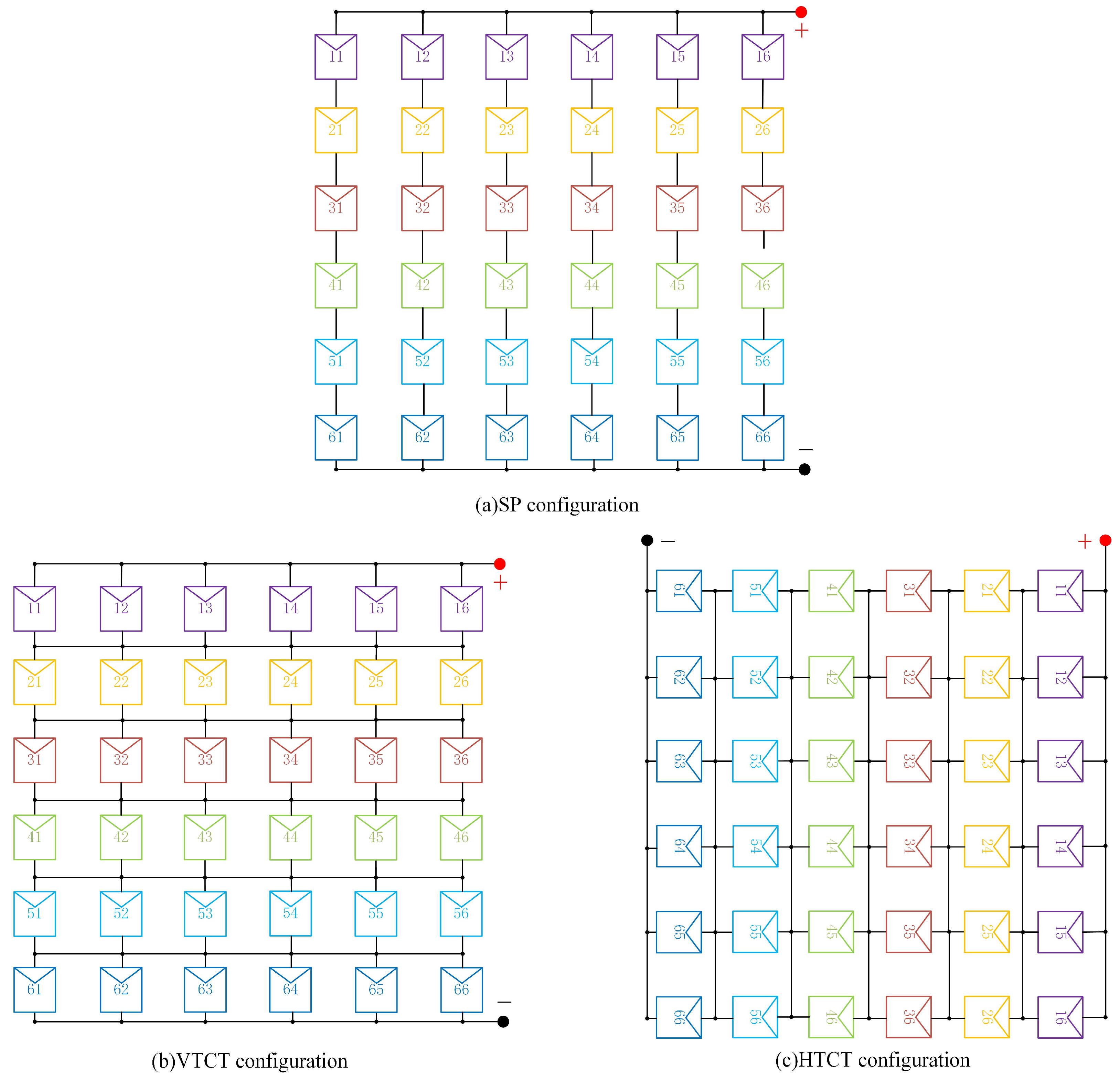
3.1. TCT Configuration

TCT configuration is realized from the series parallel configuration by connecting cross ties across each row of the junctions. Each module is designated $ij$, where $i$ is the row number and $j$ is the column number. For example, module 13 is located in the first row and third column. Applying the KVL, the array voltage $V_{PV}$ is equal to the sum of the voltages across the rows.

$$V_{PV}={\displaystyle \sum _{i=1}^m{V}_i}$$

(32)

According to KCL, the current at each node can be expressed as

$$I_a={\displaystyle \sum _{j=1}^n\left(I_{ij}-I_{\left(i+1\right)j}\right)=0}\hspace{1em}i=1,2,3,\cdots ,6$$

(33)

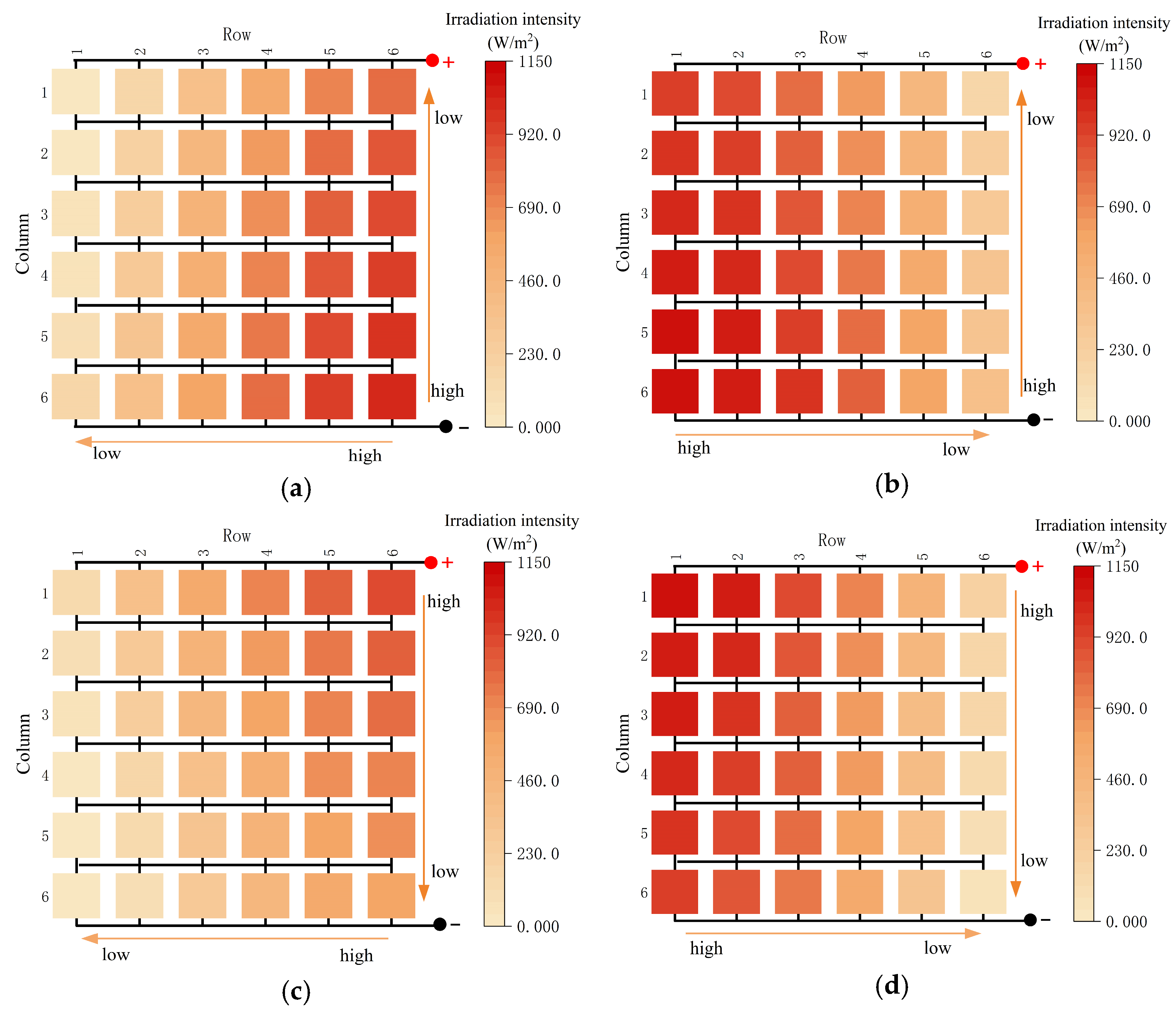
3.2. Irradiance Distribution Characteristic of PV Array

The size of airship is much larger than that of single PV module, with each module being considered a panel. The PV array of airship adopts a 6 × 6 TCT configuration, totaling 36 modules. During stable altitude cruising, the helium inside the airship’s envelope experiences superheating and overpressure due to radiant heating, resulting in regular fluctuations in pitch angle. Simultaneously, the yaw angle frequently changes in response to variations in the flight trajectory and wind conditions. The simultaneous influence of pitch angle, yaw angle and solar incidence angle results in irregular variations in the irradiance distribution of PV array. To investigate this distribution characteristics, the airspace over 23° N, 115° E is selected as a representative flying area, with the typical flight conditions specified in

Table 1. Flight conditions and attitude angles.

Condition	Date	Time	Pitch Angle	Yaw Angle
1	12.25	10:00	−8	270
2	12.25	10:00	10	10
3	12.25	10:00	8	180
4	12.25	10:00	−6	120

.

Figure 4 illustrates the irradiance distribution characteristics of the PV array corresponding for 4 different attitude angles. At a yaw angle of 270° and an angle of 10° (Figure 4a), the PV array’s irradiance intensity ranges from 7 to 1015 W/m². The sun is located in the right rear position of the airship. Consequently, the irradiance intensity decreases diagonally from right to left and from rear to front. A significant change in irradiance distribution occurs when the yaw angle shifts to 90° (Figure 4d). In this scenario, the top-left corner exhibits the highest irradiance intensity, peaking at 1100 W/m², while the bottom-right corner displays the lowest intensity at 76 W/m². Similar patterns are observed in Figure 4b,c. In Figure 4b, module 61 in the bottom-left corner demonstrates the highest irradiance intensity, whereas module 16 in the top-right corner exhibits the lowest intensity. Conversely, Figure 4c reveals an opposite pattern compared to Figure 4b.

Despite the significant and frequent variations in irradiance intensity among the airship’s PV modules, there is always a certain pattern: the irradiance intensity gradually decreases radially and circumferentially from a particular component with the highest irradiance intensity. This is a unique characteristic observed in PV arrays of airships, distinguishing them from ground-based PV systems.

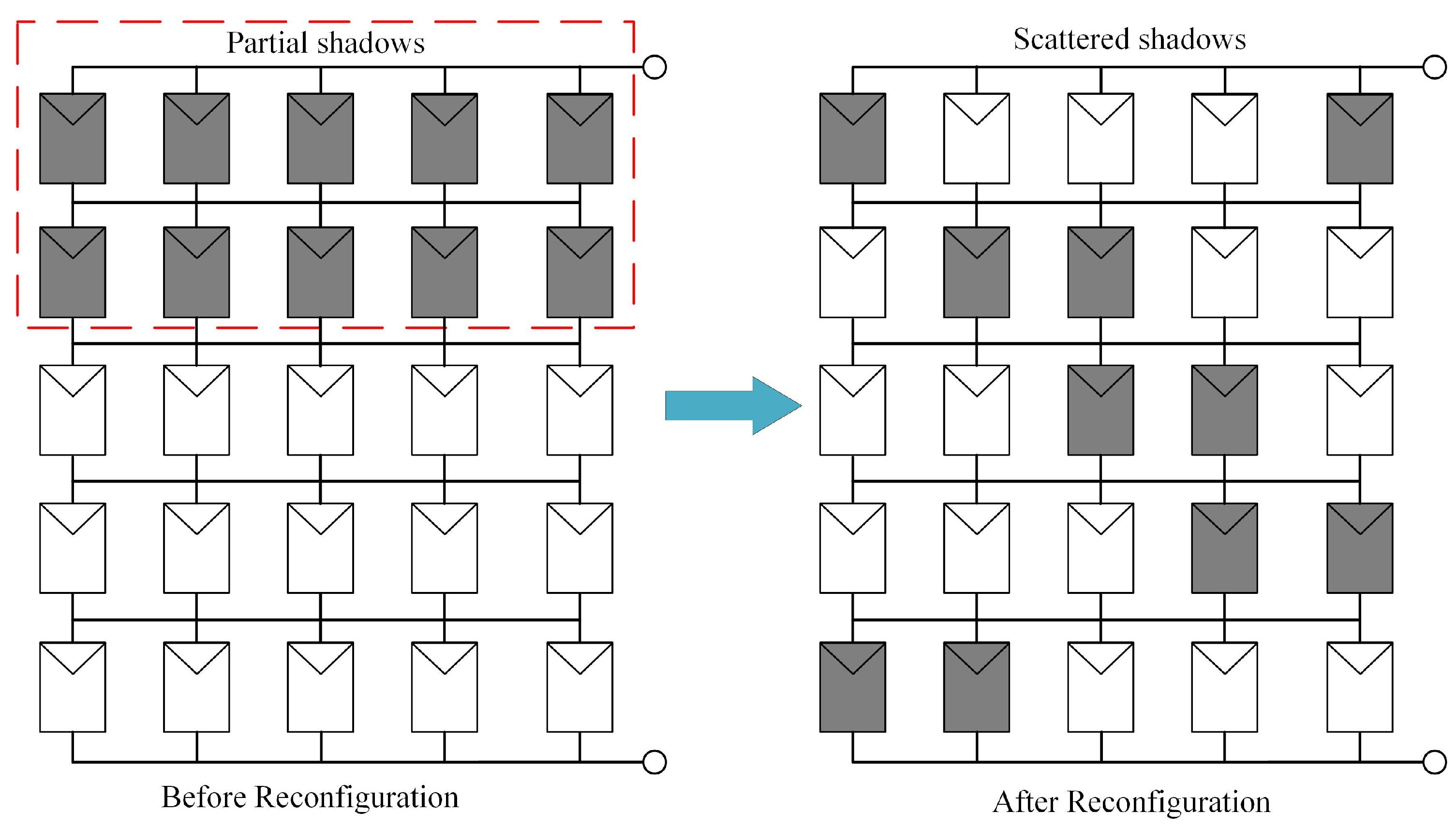
3.3. Static Reconfiguration

The non-uniformity in the sum of row irradiances is the main cause of mismatch issues of TCT configuration PV arrays. Velasco-Quesada [42] pointed out that, to maximize the available power at the PV array output, it is desirable that none of the series-connected rows of parallel-connected PV modules limit the current flowing in a single string. If the total irradiance and current of each row are equal, the mismatch loss is minimized, and the actual output power is close to the theoretical output power. Hence, the criterion for static reconfiguration of TCT-configured PV arrays is to achieve power balance among the rows by adjusting the interconnection relationships of the PV modules.

The shadows in terrestrial PV systems caused by local obstructions such as surrounding buildings and vegetation usually exhibit a concentrated distribution. This localized shading results in PV array’s mismatch loss and significantly reduces the output power. The objective of PV array static reconfiguration is to evenly disperse concentrated shadows across the entire array, thereby reducing mismatch losses. Figure 5 illustrates the distribution of shadows before and after the static reconfiguration of terrestrial PV systems. Static reconfiguration does not require additional switches or actuators, nor does it necessitate consideration of the increased cable weight cost resulting from heightened complexity of the configuration [43]. For airship PV arrays, the shadows exhibit a regular distribution, requiring a design that considers this distribution characteristic. Simultaneously, the complexity of module interconnections must be considered to minimize additional cable weight costs.

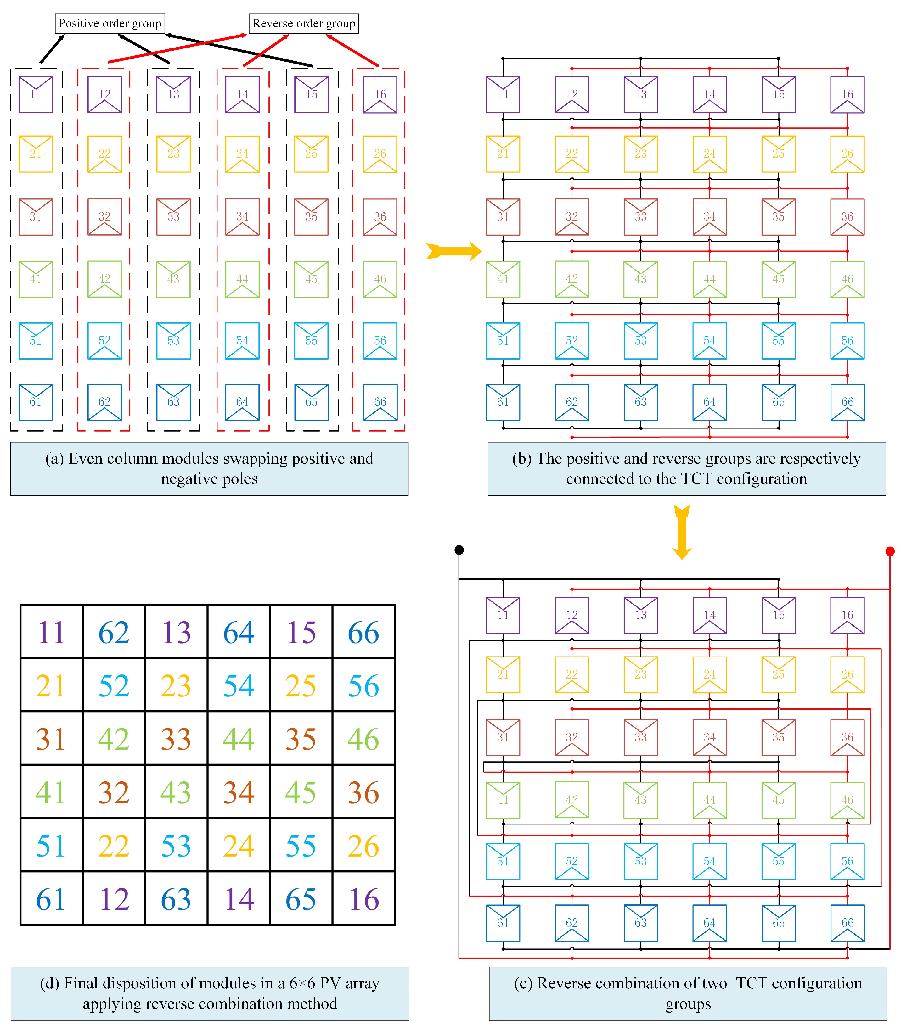
3.4. Airship PV Array Reconfiguration Technique Using Reverse Combination Method

For conventional TCT or SP connections, it is not possible to simultaneously achieve uniform radial and axial irradiance. Based on the analysis of the irradiance distribution characteristic of the PV array in Section 3.2, the irradiance of the PV array often exhibits a diagonal distribution pattern. By splitting the rows with the maximum and minimum irradiance into two interleaved parts and recombining them, the irradiance of these two rows can be made uniform. Subsequently, the same combination is applied to the rows with the second largest and second smallest irradiance, and so on, until all rows have been recombined, achieving uniform irradiance distributions in both rows and columns of the PV array. This is the “reverse combination” (RC) configuration proposed for stratospheric airship PV arrays. A 6 × 6 TCT PV array is chosen as the object of reconfiguration. Each module in the array is established by the index ‘ij’. For illustration, ‘34’ represents the module in the third row and fourth column. The given 6 × 6 square array undergoes static reconfiguration through four key steps by RC configuration.

Step 1: First, the positions of PV modules in the odd-numbered columns remain unchanged. The positive and negative polarities of the modules in the even-numbered columns are rotated to be opposite to those in the odd-numbered columns, while keeping the layout of the components unchanged, as shown in Figure 6a. The entire array is then divided into two groups: the positive order group and the reverse order group. Each group is a 6 × 3 array comprising a total of 18 modules and arranged with column spacing.

Step 2: The positive-order group and the reverse-order group are interconnected as TCT configurations, as presented in Figure 6b. These two TCT configurations are completely opposite. For the positive-order group, the first row corresponds to module 11, and its positive pole is connected to positive busbar of the array. Module 61’s negative terminal is connected to the negative busbar. Conversely, for the reverse group, module 62’s positive terminal is connected to the positive busbar, and component 12’s negative terminal is connected to the negative busbar.

Step 3: Connect the same row buses of the positive-order group and the reverse-order group separately. For example, the positive busbar of module 11 is connected to the positive busbar of module 62, the positive busbar corresponding to module 21 is connected to the positive busbar corresponding to module 52, and so on, until all the busbars of the two groups are connected. The final interconnection state is shown in Figure 6c. The row consisting of modules ‘11’, ‘62’, ‘13’, ‘64’, ‘15’, and ‘66’ is considered the first row of the configurated PV array, with the corresponding positive busbar being the PV array’s positive busbar. Modules ‘61’, ‘12’, ‘63’, ‘14’, ‘65’, and ‘16’ are the last rows of the PV array, and the corresponding negative bus is the negative bus of the array.

4. Simulation Results and Discussion

The performance of the RC configuration is evaluated by analyzing various irradiance distribution patterns. The computational results are compared to the TCT, an SP based on the PV array’s output power. A 6 × 6 PV array model is developed using the MATLAB/SIMULINK (R2020a) platform. The characteristic curve, mismatch loss power, and fill factor of the PV array are analyzed to validate the RC’s advanced configuration. Furthermore, simulations are conducted under real flight conditions, comparing the cumulative output energy to the TCT and SP configurations.

4.1. Analysis of the Performance of the Reverse Combination (RC) Configuration

4.1.1. Characteristic Curves

Figure 7 demonstrates the conventional configurations of the PV array on the airship: SP, Vertical TCT (VTCT), and Horizontal TCT (HTCT). To demonstrate the advantages of the RC, a comparative analysis is conducted on the characteristic curves with SP, VTCT, and HTCT. Typical operating conditions from

Table 2. Parameters for PV module.

Parameter	Value
Maximum power	6477.6 W
$\mathrm{Open}\mathrm{circuit}\mathrm{voltage}{V}_{oc}$	133.5 V
$\mathrm{Short}\mathrm{circuit}\mathrm{current}{I}_{sc}$	67.36 A
$\mathrm{Maximum}\mathrm{power}\mathrm{point}\mathrm{voltage}{V}_{mp}$	105.3 V
$\mathrm{Maximum}\mathrm{power}\mathrm{point}\mathrm{current}{I}_{mp}$	61.52 A
$\mathrm{Temperature}\mathrm{coefficient}\mathrm{of}{V}_{oc}$	−0.363%/°C
Temperature coefficient of $I_{sc}$	−0.0843%/°C
$\mathrm{Shunt}\mathrm{resistance}{R}_{sh}$	968.6 Ω
$\mathrm{Series}\mathrm{resistance}{R}_s$	0.58 Ω

are taken into consideration, and the corresponding I-V curves and P-V curves were simulated for the four configurations. The simulation results are depicted in Figure 8. The main parameters of the PV module under standard test conditions (STC) are shown in Table 2, and the area of the PV module is 32 m². The PV array operates at an altitude of 20 km, and the environmental temperature is set to −80 °C.

For operating condition 1, based on Figure 8a,b, the maximum output powers of the PV array are as follows: SP—98.4 kW, VTCT—102.7 kW, HTCT—81.2 kW, and RC—118.3 kW. The HTCT configuration arranges the rows of the PV modules along the airship axis. The variation in irradiance between rows is primarily influenced by yaw angle and circumferential curvature, resulting in the poorest uniformity of row irradiance and the highest level of mismatch losses. This also leads to the presence of three distinct local MPPs. In contrast, the SP and VTCT configurations arrange the modules radially along the airship, resulting in lower irradiance variations between rows due to the radial curvature and pitch angle. However, there are still mismatch losses and two local MPPs. The RC configuration performs optimally, exhibiting smooth I-V and P-V curves, and achieving the highest maximum power among the array curves. This configuration is based on the reconfiguration of VTCT and minimizes the variation in irradiance between rows caused by the longitudinal curvature and pitch angle, thereby minimizing mismatch losses.

Similar results are observed for condition 2 (Figure 8c,d), condition 3 (Figure 8e,f), and condition 4 (Figure 8g,h). In all three conditions, the RC method demonstrates an obvious advantage with output powers of 145.3 kW, 92.6 kW, and 152.2 kW, respectively. These values are 8.3%, 28%, and 14.8% higher than the second-best VTCT configuration. Furthermore, a noticeable difference in the smoothness of the I-V and P-V curves for the RC configuration can be clearly observed compared with the other three configurations.

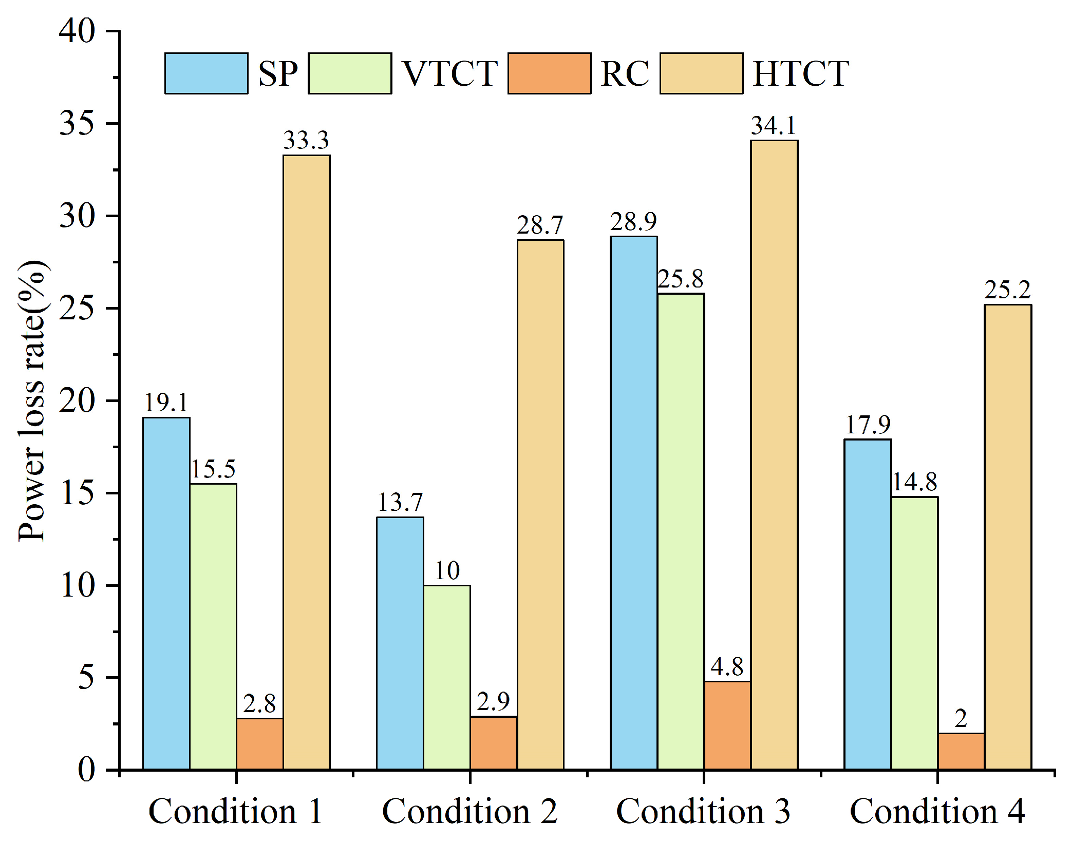
4.1.2. Mismatch Loss Power

Mismatch loss is defined as the difference between the sum of the theoretical maximum output powers of each module under the current irradiation conditions and the sum of the maximum possible output power of the PV array, which can be given by

$$P_{\mathrm{mis}}={\displaystyle \sum _j^n{\displaystyle \sum _i^m{P}_{ij,MPP} - }}{P}_{array,GMPP}$$

(34)

The maximum theoretical output power and mismatch losses are calculated for four conditions using Equation (34). Figure 9 and Figure 10 present the statistical results for the mismatch loss power and power loss rate, respectively. The RC configuration demonstrates the lowest mismatch loss powers of 3.4 kW, 4.3 kW, 4.7 kW, and 3.1 kW, which are only 3% to 5% lower than the theoretical maximum output. This is attributed to the RC configuration’s ability to achieve uniform irradiance along both the axial and radial directions of the airship array. As a result, the RC configuration exhibits a distinct advantage in terms of the array power retention rate.

4.1.3. Fill Factor (FF)

The FF is a crucial indicator used to measure the efficiency of solar cell outputs. It is determined by the ratio between the product of the open-circuit voltage and short-circuit current of the array and the maximum power of the array. A higher fill factor indicates the superior quality of the solar cell array. The calculation formula is as follows [44]:

$$FF=\frac{V_{mp}\times I_{mp}}{V_{oc}\times I_{sc}}$$

(35)

Figure 11 illustrates a comparison of the FF for 4 configurations: SP, VTCT, RC, and HTCT. The results indicate that the proposed RC configuration significantly increases the FF value. Furthermore, under various operating conditions, the PV array’s FF remains stable at approximately 0.74, which is close to the theoretical optimum value.

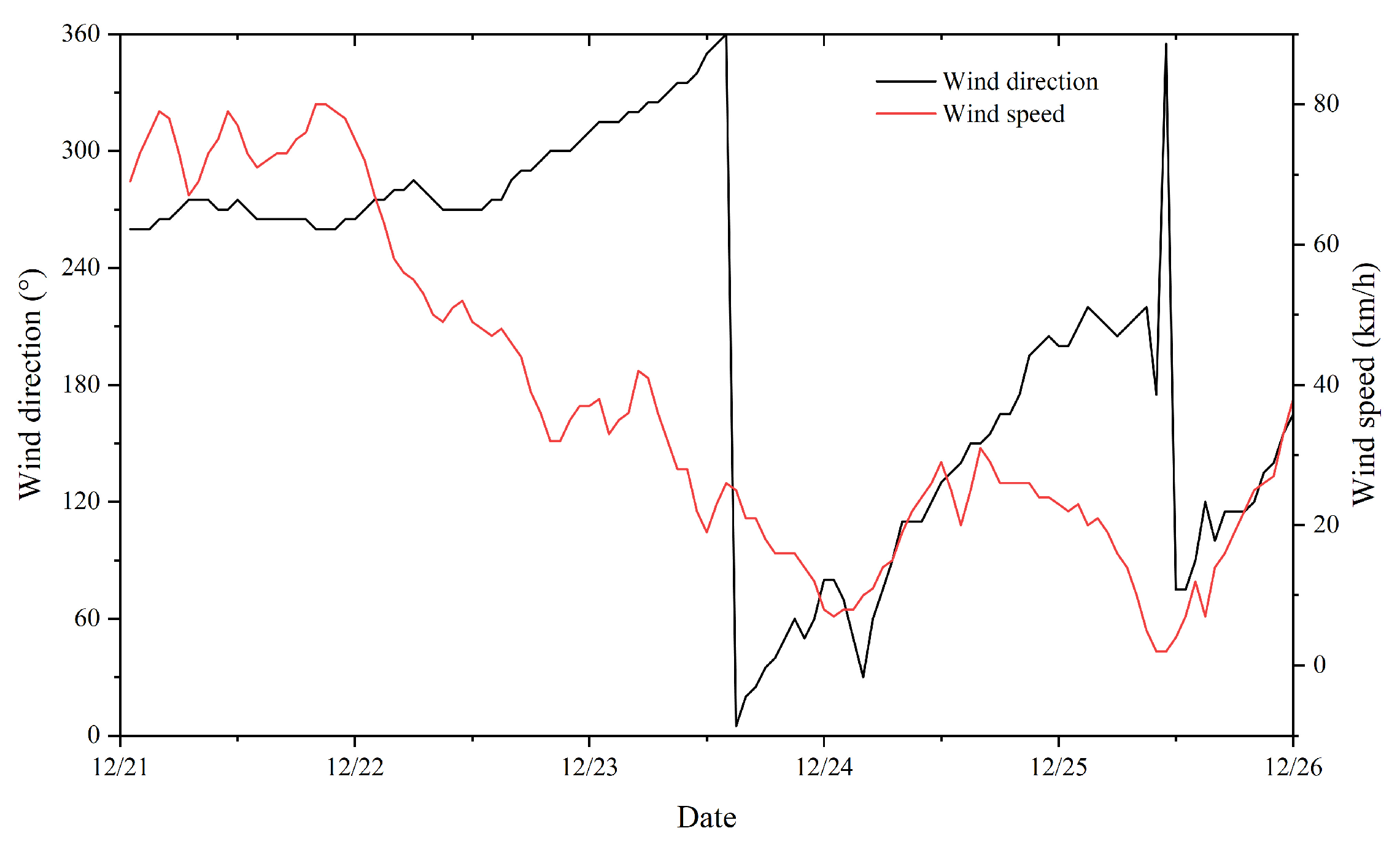
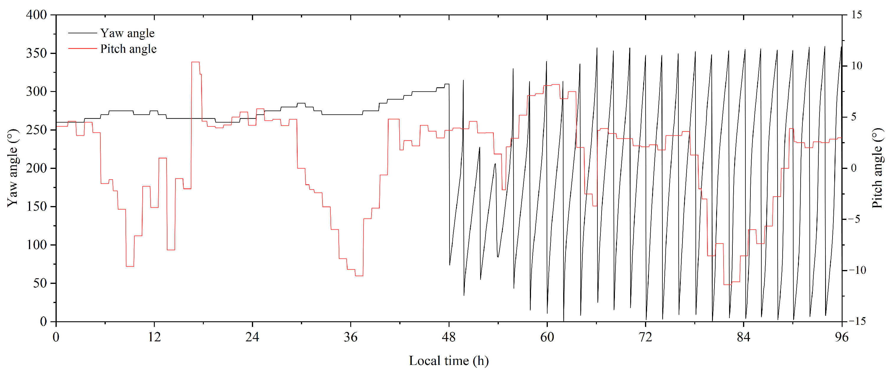
4.2. Simulation of Flight Cruising in a Real Wind Field

4.2.1. Flight Condition

Airships typically cruise at a fixed altitude with a constant roll angle. In this paper, the cruising altitude of the airship is set to 20 km, and the roll angle is set to 0°. The pitch angle oscillates according to the wind conditions and differential pressure on the envelope and is set within the range of −10° to 10°.

The cruising dates selected are from 21 December to 24 December, which correspond to the period with the lowest solar irradiance during the year. The variations in wind speed and wind direction are depicted in Figure 12, and the variations of the pitch angle and yaw angle are depicted in Figure 13. On 21 December and 22 December, the average wind speed exceeds 60 km/h, while the wind direction undergoes a shift from 250° to 0°. Therefore, the airship’s maneuvering strategy is set to resist the wind and remain in position, always facing the incoming flow to minimize energy consumption. Subsequently, on the following two days, there is a significant decrease in wind speed, with an average below 40 km/h, and the wind direction varies between 0° and 200°. With the wind speed decreasing, the airship’s cruise strategy was switched from maintaining its position to circular cruising. The cruising radius is set to 20 km, and the cruising cycle is established to be 2 h.

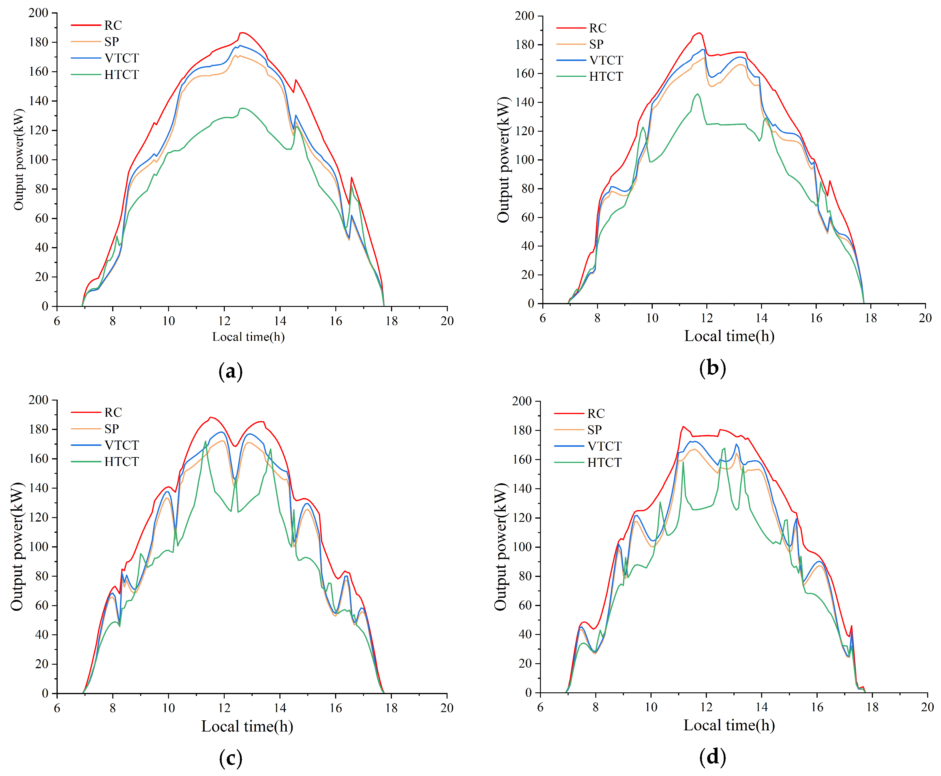
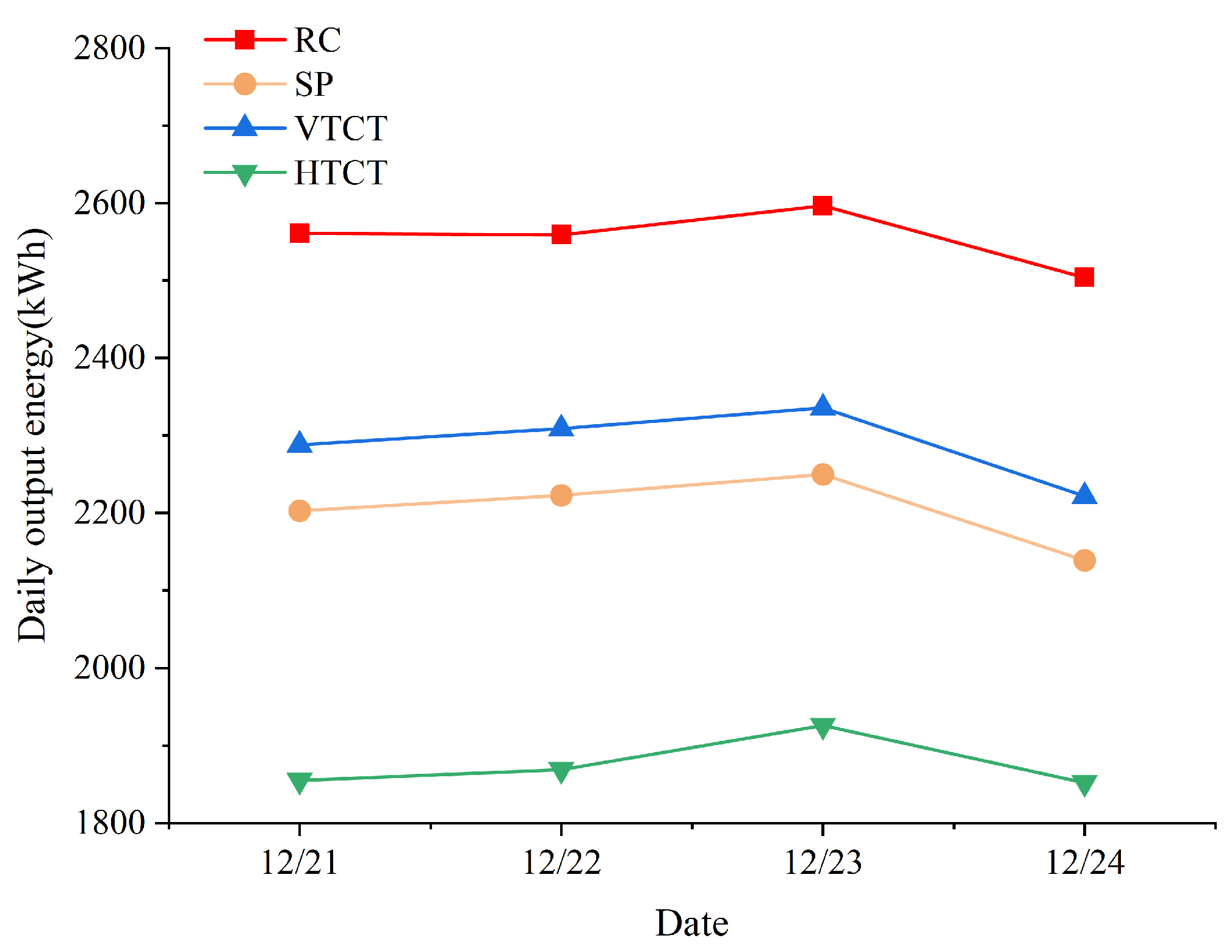
4.2.2. Comparison of Energy Generation

Figure 14a,b illustrate the electricity generation of the PV array for the two-day wind-resistance strategy. The red, blue, yellow, and green lines represent the RC, SP, VTCT, and HTCT, respectively. With this strategy, the airship exhibits minimal yaw angle variation, resulting in a stable output power curve for the array. The airship experiences minimal variation in yaw angle, and the output power of the PV array is relatively stable. On 21 December, the PV array began generating electricity at 7:00, reaching maximum power at approximately 13:00, with values of 186.5 kW, 171.2 kW, 177.8 kW, and 135.2 kW for the RC, SP, VTCT, and HTCT, respectively. Electricity generation ceased at 17:50, with the RC maintaining the highest output power throughout the day. Notably, the RC configuration showed significant improvement during the time periods of 9:00 to 11:00 and 14:00 to 16:00. This can be attributed to lower solar altitude and the airship’s curvature, resulting in significant differences in the irradiance distribution along the axial and radial. Due to rapid changes in pitch angles, all configurations experienced fluctuations at 14:20 and 16:50. Figure 14b exhibits the same pattern. It is worth noting that on both days of the simulation, the HTCT configuration consistently exhibited the lowest output power. Configurations with row modules arranged radially on the airship are inferior and unsuitable for airship PV array deployment.

The PV array exhibits more pronounced fluctuations in output power during the circular cruising strategy compared to wind resistance, as depicted in Figure 14c,d. On 23 December, with periodic changes in the roll angle, the output curves of the SP and VTCT configurations show significant power dips, occurring 7 times and aligning with the airship’s cruising cycle. Conversely, the HTCT configuration exhibits opposite fluctuations. The RC configuration maintains a stable power output, with only a minor power fluctuation occurring at 13:00, and the output power remains at its maximum throughout the entire irradiation process. Additionally, the RC configuration performs even better on 24 December, with no power fluctuations observed throughout the full irradiation period, despite other configurations still experiencing significant cyclic fluctuations, while maintaining the optimal output power consistently. For circular cruising, the RC configuration not only enhances the output power of the PV array but also improves the stability of the PV array’s output. Furthermore, it is evident that the yaw angle has a greater impact on the output power than the roll angle during the cruising mode.

Figure 15 presents the daily energy generation of the four configurations. The RC configuration consistently demonstrates the highest performance level throughout the four-day flight period. The total energy output amounts to 10,220 kWh, surpassing the VTCT configuration by 10.6%, the SP configuration by 13.8%, and the HTCT configuration by 26.6%. This significant improvement enhances the power supply capability of the PV array, thus confirming the superiority of the proposed RC configuration. The introduced RC configuration offers a promising solution to mitigate the energy shortage issue during months with low irradiation, providing valuable insights for the design of stratospheric airship PV arrays of stratospheric airships.

5. Conclusions

In this paper, we propose a novel RC configuration that involves dividing the PV array into two groups arranged in forward and reverse and recombining them to homogenize both the row and column irradiance of the airship PV array. This approach aims to reduce mismatch losses and enhance the output power of the PV array. Through simulation verification, it has been demonstrated that the proposed RC configuration effectively improves the output power of the airship photovoltaic array compared to the traditional TCT and SP configurations. Additionally, the issue of local maximum power points caused by variations in irradiance distribution are eliminated. The main conclusions can be summarized as follows:

(1)

The irradiance of the PV array exhibits a radial and circumferential gradient along the stratospheric airship. This gradient distribution varies systematically with the pitch and yaw angles. The non-uniformity in the irradiance distribution across the array leads to mismatch losses and significantly impacts the power output of the PV array.

(2)

The RC configuration optimizes the distribution of irradiance by combining adjacent column components in reverse order. This approach reduces the differences in irradiance among the row components of the array, thereby decreasing mismatch losses. Simulation results demonstrate that the RC configuration significantly enhances the output power of the PV array and eliminates localized MPP on the P-V curve.

(3)

The performance of the RC configuration surpasses that of the SP, HTCT, and VTCT configurations. It achieves the highest output power during the entire day’s operation. The net energy accumulated on the four days is 10.6% higher than the suboptimal HTCT configuration. Implementing this configuration can alleviate to some extent the energy shortage issue during weak irradiance flight conditions.

For airships with frequent variations in attitude angles, the performance of the RC configuration surpasses that of the TCT and SP configurations. However, the increased complexity of the RC configuration system and the additional mass of cables and structural attachments it brings have not been evaluated. In future work, we would like to conduct ground-scale experiments to validate the effectiveness of the proposed RC configuration and assess the cost of additional weight. Additionally, we intend to extend this configuration to other solar-powered aerial vehicles, such as solar drones and high-altitude balloons.

References

1. Schmidt, D.K.; Stevens, J.; Roney, J. Near-space station-keeping performance of a large high-altitude notional airship. J. Aircr. 2007, 44, 611–615. [Google Scholar] [CrossRef]
2. Manikandan, M.; Pant, R.S. Research and advancements in hybrid airships—A review. Prog. Aerosp. Sci. 2021, 127, 100741. [Google Scholar]
3. Zhang, J.; Xuan, Y.; Yang, L. A novel choice for the photovoltaic–thermoelectric hybrid system: The perovskite solar cell. Int. J. Energy Res. 2016, 40, 1400–1409. [Google Scholar] [CrossRef]
4. Zhang, L.C.; Lv, M.Y.; Zhu, W.Y.; Du, H.F.; Meng, J.H.; Li, J. Mission-based multidisciplinary optimization of solar-powered hybrid airship. Energy Convers. Manag. 2019, 185, 44–54. [Google Scholar] [CrossRef]
5. Pande, D.; Verstraete, D. Impact of solar cell characteristics and operating conditions on the sizing of a solar powered nonrigid airship. Aerosp. Sci. Technol. 2018, 72, 353–363. [Google Scholar] [CrossRef]
6. Li, J.; Lv, M.; Tan, D.; Zhu, W.; Sun, K.; Zhang, Y. Output performance analyses of solar array on stratospheric airship with thermal effect. Appl. Therm. Eng. 2016, 104, 743–750. [Google Scholar] [CrossRef]
7. Du, H.F.; Zhu, W.Y.; Wu, Y.F.; Zhang, L.C.; Li, J.; Lv, M.Y. Effect of angular losses on the output performance of solar array on long-endurance stratospheric airship. Energy Convers. Manag. 2017, 147, 135–144. [Google Scholar] [CrossRef]
8. Durisch, W.; Bitnar, B.; Mayor, J.C.; Kiess, H.; Lam, K.H.; Close, J. Efficiency model for photovoltaic modules and demonstration of its application to energy yield estimation. Sol. Energy Mater. Sol. Cells 2007, 91, 79–84. [Google Scholar] [CrossRef]
9. Yang, X.X.; Liu, D.N. Renewable power system simulation and endurance analysis for stratospheric airships. Renew. Energy 2017, 113, 1070–1076. [Google Scholar] [CrossRef]
10. Gonzalo, J.; López, D.; Domínguez, D.; García, A.; Escapa, A. On the capabilities and limitations of high altitude pseudo-satellites. Prog. Aerosp. Sci. 2018, 98, 37–56. [Google Scholar] [CrossRef]
11. Wang, Q.; Chen, J.; Fu, G.; Duan, D.; Zhao, H. A methodology for optimisation design and analysis of stratosphere airship. Aeronaut. J. 2009, 113, 533–540. [Google Scholar] [CrossRef]
12. Zhang, L.C.; Lv, M.Y.; Meng, J.H.; Du, H.F. Optimization of solar-powered hybrid airship conceptual design. Aerosp. Sci. Technol. 2017, 65, 54–61. [Google Scholar] [CrossRef]
13. Meng, J.H.; Liu, S.Y.; Yao, Z.B.; Lv, M.Y. Optimization design of a thermal protection structure for the solar array of stratospheric airships. Renew. Energy 2019, 133, 593–605. [Google Scholar] [CrossRef]
14. Lv, M.; Li, J.; Du, H.; Zhu, W.; Meng, J. Solar array layout optimization for stratospheric airships using numerical method. Energy Convers. Manag. 2017, 135, 160–169. [Google Scholar] [CrossRef]
15. Alam, M.I.; Pant, R.S. Multi-objective multidisciplinary design analyses and optimization of high altitude airships. Aerosp. Sci. Technol. 2018, 78, 248–259. [Google Scholar] [CrossRef]
16. Jiang, Y.; Lv, M.; Sun, K. Effects of installation angle on the energy performance for photovoltaic cells during airship cruise flight. Energy 2022, 258, 124982. [Google Scholar] [CrossRef]
17. Wang, H.F.; Song, B.F.; Zuo, L.K. Effect of high-altitude airship’s attitude on performance of its energy system. J. Aircr. 2007, 44, 2077–2080. [Google Scholar] [CrossRef]
18. Zhu, W.Y.; Li, J.; Xu, Y.M. Optimum attitude planning of near-space solar powered airship. Aerosp. Sci. Technol. 2019, 84, 291–305. [Google Scholar] [CrossRef]
19. Zhang, L.C.; Li, J.; Wu, Y.F.; Lv, M.Y. Analysis of attitude planning and energy balance of stratospheric airship. Energy 2019, 183, 1089–1103. [Google Scholar] [CrossRef]
20. Shan, C.; Lv, M.Y.; Sun, K.W.; Gao, J. Analysis of energy system configuration and energy balance for stratospheric airship based on position energy storage strategy. Aerosp. Sci. Technol. 2020, 101, 105844. [Google Scholar] [CrossRef]
21. Quesada, G.; Guillon, L.; Rousse, D.R.; Mehrtash, M.; Dutil, Y.; Paradis, P.L. Tracking strategy for photovoltaic solar systems in high latitudes. Energy Convers. Manag. 2015, 103, 147–156. [Google Scholar] [CrossRef]
22. Hu, Y.G.; Yao, Y.X. A methodology for calculating photovoltaic field output and effect of solar tracking strategy. Energy Convers. Manag. 2016, 126, 278–289. [Google Scholar] [CrossRef]
23. Lv, M.; Li, J.; Zhu, W.; Du, H.; Meng, J.; Sun, K. A theoretical study of rotatable renewable energy system for stratospheric airship. Energy Convers. Manag. 2017, 140, 51–61. [Google Scholar] [CrossRef]
24. Du, H.F.; Li, J.; Zhu, W.Y.; Yao, Z.B.; Cui, E.Q.; Lv, M.Y. Thermal performance analysis and comparison of stratospheric airships with rotatable and fixed photovoltaic array. Energy Convers. Manag. 2018, 158, 373–386. [Google Scholar] [CrossRef]
25. Zhu, W.Y.; Xu, Y.M.; Li, J.; Zhang, L.C. Performance analysis of rotatable energy system of high-altitude airships in real wind field. Aerosp. Sci. Technol. 2020, 98, 105689. [Google Scholar] [CrossRef]
26. Liu, Y.; Sun, K.; Xu, Z.; Lv, M. Energy efficiency assessment of photovoltaic array on the stratospheric airship under partial shading conditions. Appl. Energy 2022, 325, 119898. [Google Scholar] [CrossRef]
27. Belhachat, F.; Larbes, C. PV array reconfiguration techniques for maximum power optimization under partial shading conditions: A review. Sol. Energy 2021, 230, 558–582. [Google Scholar] [CrossRef]
28. Kuznetsov, P.; Yuferev, L.; Voronin, D.; Panchenko, V.A.; Jasinski, M.; Najafi, A.; Leonowicz, Z.; Bolshev, V.; Martirano, L. Methods Improving Energy Efficiency of Photovoltaic Systems Operating under Partial Shading. Appl. Sci. 2021, 11, 696. [Google Scholar] [CrossRef]
29. Rani, B.I.; Ilango, G.S.; Nagamani, C. Enhanced Power Generation From PV Array Under Partial Shading Conditions by Shade Dispersion Using Su Do Ku Configuration. IEEE Trans. Sustain. Energy 2013, 4, 594–601. [Google Scholar] [CrossRef]
30. Venkateswari, R.; Rajasekar, N. Power enhancement of PV system via physical array reconfiguration based Lo Shu technique. Energy Convers. Manag. 2020, 215, 112885. [Google Scholar] [CrossRef]
31. Nasiruddin, I.; Khatoon, S.; Jalil, M.F.; Bansal, R.C. Shade diffusion of partial shaded PV array by using odd-even structure. Sol. Energy 2019, 181, 519–529. [Google Scholar] [CrossRef]
32. Madhusudanan, G.; Senthilkumar, S.; Anand, I.; Sanjeevikumar, P. A shade dispersion scheme using Latin square arrangement to enhance power production in solar photovoltaic array under partial shading conditions. J. Renew. Sustain. Energy 2018, 10, 053506. [Google Scholar] [CrossRef]
33. Wu, J.T.; Fang, X.D.; Wang, Z.G.; Hou, Z.X.; Ma, Z.Y.; Zhang, H.L.; Dai, Q.M.; Xu, Y. Thermal modeling of stratospheric airships. Prog. Aerosp. Sci. 2015, 75, 26–37. [Google Scholar] [CrossRef]
34. Yao, W.; Lu, X.C.; Wang, C.; Ma, R. A heat transient model for the thermal behavior prediction of stratospheric airships. Appl. Therm. Eng. 2014, 70, 380–387. [Google Scholar] [CrossRef]
35. El Mghouchi, Y.; Chham, E.; Krikiz, M.S.; Ajzoul, T.; El Bouardi, A. On the prediction of the daily global solar radiation intensity on south-facing plane surfaces inclined at varying angles. Energy Convers. Manag. 2016, 120, 397–411. [Google Scholar] [CrossRef]
36. Shan, C.; Sun, K.; Ji, X.; Cheng, D. A reconfiguration method for photovoltaic array of stratospheric airship based on multilevel optimization algorithm. Appl. Energy 2023, 352, 121881. [Google Scholar] [CrossRef]
37. Li, J.; Liao, J.; Liao, Y.X.; Du, H.F.; Luo, S.B.; Zhu, W.Y.; Lv, M.Y. An approach for estimating perpetual endurance of the stratospheric solar-powered platform. Aerosp. Sci. Technol. 2018, 79, 118–130. [Google Scholar] [CrossRef]
38. Wang, J.; Meng, X.Y.; Li, C.C.; Qiu, W.J. Analysis of long-endurance station-keeping flight scenarios for stratospheric airships in the presence of thermal effects. Adv. Space Res. 2021, 67, 4121–4141. [Google Scholar] [CrossRef]
39. Ram, J.P.; Manghani, H.; Pillai, D.S.; Babu, T.S.; Miyatake, M.; Rajasekar, N. Analysis on solar PV emulators: A review. Renew. Sustain. Energy Rev. 2018, 81, 149–160. [Google Scholar] [CrossRef]
40. Gupta, J.; Hussain, A.; Singla, M.K.; Nijhawan, P.; Haider, W.; Kotb, H.; AboRas, K.M. Parameter Estimation of Different Photovoltaic Models Using Hybrid Particle Swarm Optimization and Gravitational Search Algorithm. Appl. Sci. 2023, 13, 249. [Google Scholar] [CrossRef]
41. Dimara, A.; Papaioannou, A.; Grigoropoulos, K.; Triantafyllidis, D.; Tzitzios, I.; Anagnostopoulos, C.-N.; Krinidis, S.; Ioannidis, D.; Tzovaras, D. A Novel Real-Time PV Error Handling Exploiting Evolutionary-Based Optimization. Appl. Sci. 2023, 13, 12682. [Google Scholar] [CrossRef]
42. Velasco, G.; Guinjoan, F.; Pique, R. Grid-Connected PV Systems Energy Extraction Improvement by means of an Electric Array Reconfiguration (EAR) Strategy: Operating Principle and Experimental Results. In Proceedings of the 39th IEEE Power Electronics Specialists Conference (PESC 08), Rhodes Isl, Greece, 15–19 June 2008; pp. 1983–1988. [Google Scholar]
43. Dhanalakshmi, B.; Rajasekar, N. A novel Competence Square based PV array reconfiguration technique for solar PV maximum power extraction. Energy Convers. Manag. 2018, 174, 897–912. [Google Scholar] [CrossRef]
44. Sarniak, M.T. Modeling the Functioning of the Half-Cells Photovoltaic Module under Partial Shading in the Matlab Package. Appl. Sci. 2020, 10, 2575. [Google Scholar] [CrossRef]
Figure 1. Schematic diagram of stratospheric airship PV array [36].
Applsci 14 00747 g001
Figure 2. Schematic of θ D I P .
Applsci 14 00747 g002
Figure 3. Single-diode model of solar cell.
Applsci 14 00747 g003
Figure 4. Irradiance distribution characteristics: (a) condition 1; (b) condition 2; (c) condition 3; (d) condition 4.
Applsci 14 00747 g004
Figure 5. Static terrestrial PV Array reconfiguration.
Applsci 14 00747 g005
Figure 6. Implementation of reverse combination method step in a 6 × 6 PV array.
Applsci 14 00747 g006
Figure 7. Diagram of SP, VTCT, and HTCT.
Applsci 14 00747 g007
Figure 8. Characteristic curves for SP, VTCT, RC and HTCT: (a) I-V curve for condition 1; (b) P-V curve for condition 1; (c) I-V curve for condition 2; (d) P-V curve for condition 2; (e) I-V curve for condition 2; (f) P-V curve for condition 2; (g) I-V curve for condition 2; (h) P-V curve for condition 2.
Applsci 14 00747 g008
Figure 9. Mismatch loss power for conditions 1 to 4.
Applsci 14 00747 g009
Figure 10. Power loss rates for conditions 1 to 4.
Applsci 14 00747 g010
Figure 11. Estimation of fill factors for conditions 1 to 4.
Applsci 14 00747 g011
Figure 12. Wind speed and direction from 21 December to 25 December.
Applsci 14 00747 g012
Figure 13. Yaw angle and Pitch angle from 21 December to 25 December.
Applsci 14 00747 g013
Figure 14. Comparison of output power during daytime: (a) 21 December; (b) 22 December; (c) 23 December; (d) 24 December.
Applsci 14 00747 g014
Figure 15. Comparison of daily output energy.
Applsci 14 00747 g015