Abstract
Within the strain level attainable in drained triaxial tests, it is not uncommon for dense cohesionless soil to be sheared insufficiently to reach the critical state. Linear fitting of the correlative data from the maximum stress ratio or minimum dilatancy to the end of the test, and then extrapolating these fitted lines to the critical stress ratio or zero dilatancy has been frequently used to estimate the critical state void ratio. However, the linear extrapolation method is empirical and involves different choices of correlative test data, which leads to different estimates. Therefore, a series of simulations of drained tests on dense Toyoura sand are performed using a state-dependent model. Multiple data sets are generated, including void ratio e, volumetric strain εv, stress ratio η, and dilatancy D. The linear extrapolation accuracy of the e–η, e–D, and εv–D data sets is examined. It turns out that the e–η data set is best suited. The goodness of the e–η data set is examined against 18 sets of experimental data on dense sand. In addition, the selection of the start point for extrapolation is shown to influence the estimates. The latter 50% of the post-peak data is found to be reliable.
1. Introduction
The term critical state is defined as a limit state in which a soil element continues to deform at constant void ratio (or volumetric strain), mean effective stress, and deviatoric stress [1,2,3,4]. Poorooshasb [5] defined this state symbolically as
where εq, e, εv, p, q, and η (=q/p) are the deviatoric strain, void ratio, volumetric strain, mean effective stress, deviatoric stress, and stress ratio of the soil element, respectively.
The concept of critical state is well accepted and understood in soil mechanics [6,7,8,9,10,11] and rock mechanics [12,13]. This concept is also considered to have applications to new types of composite geo-materials in civil engineering, such as soil–waste mixtures [14,15].
It is not unusual to use standard drained triaxial compression tests (in which dq/dp = 3 and εq = εa − εv/3, where εa is the axial strain) to obtain the critical state locus in the confinement–shear–volume (p–q–e) space [4,14,16]. The locus is normally characterized using a linear failure envelope in the q–p plane and a critical state line in the e–p plane. The slope of the failure envelope, qcs/pcs (where the subscript cs indicates ‘critical state’), is called the critical state stress (or friction) ratio ηcs, which is often denoted by M. The critical state line depicts the relationship between the void ratio at the critical state ecs and the corresponding mean effective stress pcs.
For dense (‘dilative’) cohesionless granular geo-materials, the critical state is typically attained at large strains upon the end of the strain-softening process. As a consequence, it is not uncommon that, within the limits of the triaxial equipment, the critical state is not reached at the end of the tests (e.g., [14,17,18,19,20]). In this situation, it becomes necessary to estimate the values of ecs, pcs, and M from measured data that are free of interference from strain localization into shear bands. This interference could be minimized by utilizing the testing devices and procedures recommended by [21,22].
Three methods are available for estimating the critical state void ratio ecs or volumetric strain εvcs (which is given by ln[(1 + e0)/(1 + ecs)], where e0 is the initial (‘pre-shearing’) void ratio). The first method extrapolates the εv–εq (or εv–εa) data to a specified ‘most probable’ value of εq (or εa) postulated to be at the onset of the critical state, say, 35% [14,18,23], to an εq (or εa) value approaching infinity [24,25,26] or to an εq value estimated from extrapolation of the η–εq data to the critical state stress ratio ηcs (M) [27]. Different curve-fitting functions, data sets, and data set sizes have been used in this extrapolation, including hyperbolic [25] and exponential [26] functions for fitting the entire data, and sine functions for fitting a subset of the data from the minimum volumetric strain to the end of the test [27]. It seems that the selection of a curve-fitting function and a data set was based on personal observation and preference. The second method extrapolates the void ratio–stress ratio (e–η) trend to an estimated critical state stress ratio ηcs [28]. The e–η data set from the maximum (‘peak’) stress ratio ηmax to the end of the test is used for extrapolation. The third method extrapolates the void ratio– or volumetric strain–dilatancy (e–D or εv–D) trend to the critical state condition of a zero dilation rate D = 0, where D = d/d and the superscript p indicates the ‘plastic’ component of the strain increment [24,29,30,31]. The e–D or εv–D data set from the minimum dilation rate Dmin (because of the compression positive convention) to the end of the test is used for extrapolation. Simple linear extrapolation has been consistently adopted in the last two methods, making the methods attractive for estimating the critical state void ratio ecs. There nevertheless remains a lack of knowledge about which of the e–η, e–D, and εv–D data sets is best suited for linear extrapolation and how dependent the goodness-of-fit of the linear function is on the size (or the start point) of the data set.
In this paper, a state-dependent constitutive model for cohesionless soils developed by Li and Dafalias [32] is used to perform a series of numerical simulations of drained triaxial compression tests on Toyoura sand. Multiple sets of e, εv, η, and D data are derived from the simulations. The accuracy of the critical state void ratios estimated from linear extrapolation of the e–η, e–D, and εv–D data sets is examined. The data set best suited for linear extrapolation is determined, and then the effect of its size on the goodness of fit of the linear function is evaluated using experimental data freely available from Wichtmann’s homepage on the torsten-wichtmann.de website [33]. Guidance is obtained on the start point of the data set required to reach a certain high level of the coefficient of determination.
2. The Most Appropriate Data Set for Extrapolation
Li and Dafalias [32] proposed a fundamental model for simulating triaxial compression tests on cohesionless soils. In this model, the concept of state-dependent dilatancy was introduced, and a dilatancy function was proposed as given by
where e is Euler’s number; D0 and m are two positive model parameters; and ψ = e − ecs is the state parameter defined by Been and Jefferies [4], which measures how far the soil state under the current void ratio e and confining pressure p is from the critical state. Such defined dilatation ratio makes it possible to model the dilatancy characteristics dependent on different void ratios and pressures.
Because the e-log p plots of critical-state lines for cohesionless soil are in general not straight, Li and Wang [34] proposed a more appropriate empirical formula to depict the critical state line as
where eΓ, λc, and ξ are the material constants and pa is the atmospheric pressure (101.325 kPa), serving as a scaling factor for normalization or dimensional homogeneity.
To model the elastic behavior, shear modulus was defined as a function of not only p but also of e, as given by
where e is used instead of the initial void ratio e0 used in [35] and G0 is a dimensionless material constant. The unit of G is reflected by (ppa)0.5. Within elasticity theory, the elastic bulk modulus K is equal to
where ν is Poisson’s ratio, which was considered to be a material constant.
The yield criterion was assumed to be f = q − ηp = 0. A state-dependent plastic modulus Kp was proposed as given by
where h1 and h2 are two material constants and n is a positive model parameter. Such defined plastic modulus makes it possible to model the peak stress ratio response and strain softening of dense soils, the strain hardening of loose soils, and the failure at the critical state stress ratio M. A systematic procedure for the calibration of model parameters was also provided. Equations (7) and (8) show the relationship between the stress and strain increments of Li and Dafalias’ [32] model.
Based on the triaxial test data reported by Verdugo and Ishihara [36], Li and Dafalias [32] calibrated the model parameters for Toyoura sand as follows: G0 = 125, ν = 0.05, M = 1.25, eΓ = 0.934, λc = 0.019, ξ = 0.7, D0 = 0.88, m = 3.5, h1 = 3.15, h2 = 3.05, and n = 1.1. In the present paper, Li and Dafalias’ [32] model and parameters are used to perform a series of simulations of drained triaxial compression tests on Toyoura sand with a range of initial (‘pre-shearing’) confining pressures p0 and void ratios e0.
Figure 1 shows the critical state line of Toyoura sand under confining pressures not greater than 500 kPa. A total of 20 numerical simulations of drained shear tests on dilative sand specimens were carried out. The pre-shearing states of the specimens are shown by the abscissa and ordinate values of the solid circles in Figure 1. Each circle is numbered for ease of identification. The density index ID = (emax − e0)/(emax − emin) is used as a proxy for e0 (Toyoura sand having the maximum void ratio emax = 0.977 and the minimum void ratio emin = 0.597 [36]).
Figure 1.
The critical state line (CSL) of Toyoura sand and the pre-shearing states of the sand specimens employed in the drained shear test simulations (the CSL is based on Li and Wang’s [34] empirical formula and Li and Dafalias’ [32] parameters).
Figure 2 shows typical results obtained from the simulations of drained shear tests on Toyoura sand with a pre-shearing confining pressure p0 of 200 kPa and different density indices. The critical state stress ratio M obtained is identical to the input value of 1.25. The critical void ratio obtained, 0.8894, is also identical to the theoretical value that would be derived from traditional calculations with qcs = Mpcs = 3(pcs − p0) and ecs = eΓ − λc(pcs/pa)ξ. Figure 2a clearly shows the peak stress ratio response and the post-peak strain-softening behavior, and Figure 2b shows the dilating behavior. It is noted that none of the simulated tests attain the critical state at an axial strain εa of 25%, which is approximately the highest strain level attainable in triaxial tests. For all the simulated tests, a conservative value of the axial strain for attaining the critical state is approximately 80%. As expected, the higher the density index, the higher the axial strain necessary to attain the critical state.
Figure 2.
Results obtained from the simulations of drained shear tests on Toyoura sand with a pre-shearing confining pressure p0 of 200 kPa and different density indices ID.
The e–η data set of Toyoura sand with a pre-shearing confining pressure p0 of 200 kPa and a density index ID of 2/3 (for which e0 = 0.724) is plotted as e versus (η − M), as shown by the solid grey curve in Figure 3. For practical consideration, εa = 25% is assumed to be the end value of the experiment. A subset of the post-peak data from a specified start point to an assumed end of test at εa = 25% was fitted and extrapolated, while the simulation values ranging from 25% to 80% are used for comparison with the fitted and extrapolated curve for validation. The location of the start point is defined as
where ηEOT is the stress ratio at the end of the test; sη is expressed in percentage and indicates approximately what the percentage of the post-peak data used for extrapolation is.
Figure 3.
Performance of the linear extrapolation method for the e–η data set of Toyoura sand with p0 = 200 kPa and ID = 2/3.
A best-fit line of the e–η data from the start point at sη = 90% up to the end point at εa = 25% is shown by the dashed line in Figure 3. This line agrees excellently with the fitted data, which covers approximately ninety percent of the post-peak data. Extrapolating this line to η − M = 0 leads to an estimated critical state void ratio ecses = 0.8894, which is identical to the theoretical value of the critical state void ratio.
The colored curves in Figure 4 represent the simulation results of the e–D and εv–D data sets of Toyoura sand under the conditions p0 = 200 kPa and ID = 2/3. The relationship between e and εv is given by εv = ln[(1 + e0)/(1 + e)]. During the dilation process, e increases and D varies from a negative minimum to zero, which corresponds to the critical state condition. Best-fit lines for the data sets from the start points at sη = 90%, 70%, and 50% up to the end point at εa = 25% are shown by the dashed lines in Figure 4a–c, respectively. Extrapolating these lines to D = 0 leads to the estimated critical state void ratios ecses and volumetric strains εvcses. It can be seen that the ordinate values of the dashed lines at D = 0 are more or less higher than those of the corresponding colored curves. This indicates that the critical state void ratio and volumetric strain are overestimated by the linear extrapolation of the e–D and εv–D data sets, respectively. By comparing Figure 3 with Figure 4, it is apparent that the e–η data set is more suitable for linear extrapolation than the e–D and εv–D data sets.
Figure 4.
Performance of the linear extrapolation method for the e–D and εv–D data sets of Toyoura sand with p0 = 200 kPa and ID = 2/3.
By performing numerical simulations of 20 drained triaxial tests on Toyoura sand with different pre-shearing states designated by the solid dots in Figure 1, the e–η, e–D, and εv–D data for these sands were obtained and used to estimate their critical state void ratios with the linear extrapolation method. The absolute error of the estimated critical state void ratio ecses is defined as Ea = ecses − ecs and is used to evaluate the overall performance of the linear extrapolation method. Figure 5 shows the absolute errors of ecses generated from the linear extrapolation of the data of all twenty test simulations. The absolute error decreases as the density index ID decreases. This indicates that the denser the sand state, the lower the extrapolation accuracy. The absolute errors induced by the use of the e–D and εv–D data sets are evidently greater than those induced by the use of the e–η data set. Therefore, it can be concluded that among the three data sets, the e–η data set is best suited to estimate the critical state void ratio with linear extrapolation. Figure 5a–c show the absolute errors induced by the start points of extrapolated data located at sη = 90%, 70%, and 50%, respectively. Obviously, the selection of the start point of the data for extrapolation has an important influence on the accuracy of extrapolation. The lower the sη value is, the smaller the absolute error and the higher the extrapolation accuracy. On the other hand, the lower the sη value, the smaller the amount of data used for extrapolation. Therefore, a reasonable selection of the start point for the e–η data set should be made for extrapolation. It can be seen from Figure 5c that the absolute errors induced by the use of the e–η data from the start point at sη = 50% to the end of the test are generally under ±0.0025. In the next section, the effect of the start point on the linearity between the e and η data will be further evaluated against experimental data.
Figure 5.
The absolute errors of the estimated critical state void ratios generated from the linear extrapolation of the data of all twenty test simulations.
3. Practical Selection of the Start Point of the Data to Be Extrapolated
Wichtmann and Triantafyllidis [37] reported the experimental results obtained from multiple series of triaxial tests on Karlsruhe fine sand, which included 25 drained monotonic triaxial compression tests. The sand has almost no fine content, emin = 0.677, and emax = 1.054. The critical state friction angle was determined to be φcs = 33.1°, from which it follows that M = 6sinφcs/(3 − sinφcs) = 1.335. All test data are freely available from Wichtmann’s homepage on the torsten-wichtmann.de website [33]. Out of the 25 drained tests, 20 tests on medium-dense and dense samples showed strain-softening and dilatancy behavior. These 20 tests were numbered from TMD6 to TMD 25 by [37]. Table 1 of [37] presented the pre-shearing void ratios e0 and confining pressures p0 of the sand tested.
Figure 6 shows the e–(η − M) data obtained from the 20 tests. All the e–(η − M) curves terminate at a stress ratio η greater than the critical state stress ratio M. This indicates that their critical states were not attained. After the peak stress ratio is reached, the void ratio e increases and the stress ratio decreases, corresponding, respectively, to the dilatancy and strain-softening behavior. Relatively steady data fluctuations were observed in the later stage of tests TMD7 and TMD17, as shown in Figure 6a. Negligible data fluctuations were observed in the other 12 tests, as shown in Figure 6a,b. However, unsteady data fluctuations were observed in another six tests, as shown in Figure 6c. In these six tests, tests TMD11 and TMD16 showed evidently nonlinear e–(η − M) behavior, so they were discarded from further analysis. The remaining four tests showed short random fluctuations close to the end of the tests only. For each of the four tests, an assumed end of test was specified and used for further analysis, as shown by the symbols in Figure 6c. Therefore, a total of 18 tests were considered. It can be seen from Figure 6 that the e–(η − M) curves for these tests become approximately linear only until the stress ratio decreases to a certain value. Therefore, the entire post-peak data set cannot be used to perform linear extrapolation. The selection of a reasonable start point for the e–(η − M) data is the key to the goodness of fit for the linear extrapolation.
Figure 6.
The e–η data of the drained triaxial compression tests on medium-dense and dense Karlsruhe fine sand (data reproduced from Wichtmann’s homepage on the torsten-wichtmann.de website [33]).
Figure 7 shows the coefficients of determination (R2) of the least-squares linear fits of the e–η data from varying start points as defined by Equation (9) to the end of the test. The R2 of determination for tests TMD7, TMD12, TMD18, TMD21, and TMD 24 fluctuate relatively significantly with the change in the start point, especially when the sη value is less than 50%. For the other 13 tests, generally speaking, the coefficient of determination increases as the sη value decreases from 90% to 50%, and then it varies within a relatively narrow range as the sη value further decreases from 50% to 20%. Their coefficients of determination of the least-squares linear fits of the e–η data from the start point at sη = 50% to the end of the test are greater than 0.975. Therefore, sη = 50% may be used as a reasonable start point for fitting and extrapolating the e–η data. This means that the latter fifty percent of the post-peak e–η data may be the best option for estimating the critical state void ratio with the linear extrapolation method.
Figure 7.
The coefficients of determination (R2) of the least-squares linear fits of the e–η data from varying start points to the end of the test (the numerals indicate test numbers (TMD)).
4. Discussion
The linear extrapolation accuracy of the e–η, e–D, and εv–D data sets is examined using simulations of drained shear tests on Toyoura sand. The e–η data set is best suited, and a new recommendation of using the latter 50% of the post-peak data for extrapolation is presented. Compared with previous empirical studies, this paper complements the theoretical basis for the linear extrapolation method and points out a more accurate selection of the starting point for extrapolation. The discovery that the e–η data set is most suitable for extrapolation was achieved by examining the correlative test data simulated by a state-dependent model. Therefore, we believe that this conclusion is also applicable to other materials that can be captured by this model (e.g., rubber–sand mixtures [15,38], silty sands [39], and rockfill materials [40]). However, for the practical application of this method to these composite soils, the recommendation of using the latter 50% of the post-peak data for extrapolation must be further verified with experiments.
In addition, due to the complex mechanical properties of natural structured soil, research on soil mechanics often starts with clean remolded samples, such as the development of critical state soil mechanics and the Cam-clay model [2,3] and the state-dependent model [32]. The influence of structure can be further incorporated based on remolded soil theories [41]. Therefore, the application of this method to natural structured soil deserves further investigation and modification in the future.
5. Conclusions
Critical state theory is the cornerstone of modern soil mechanics [2]. This paper aims to find the best choice of correlative test data for extrapolating the critical state void ratio of cohesionless soil. The extrapolated critical state void ratio can be used in the determination of CSL and further geotechnical engineering applications. Based on the analyses of simulation data and experimental data, the following conclusions can be drawn:
- (a)
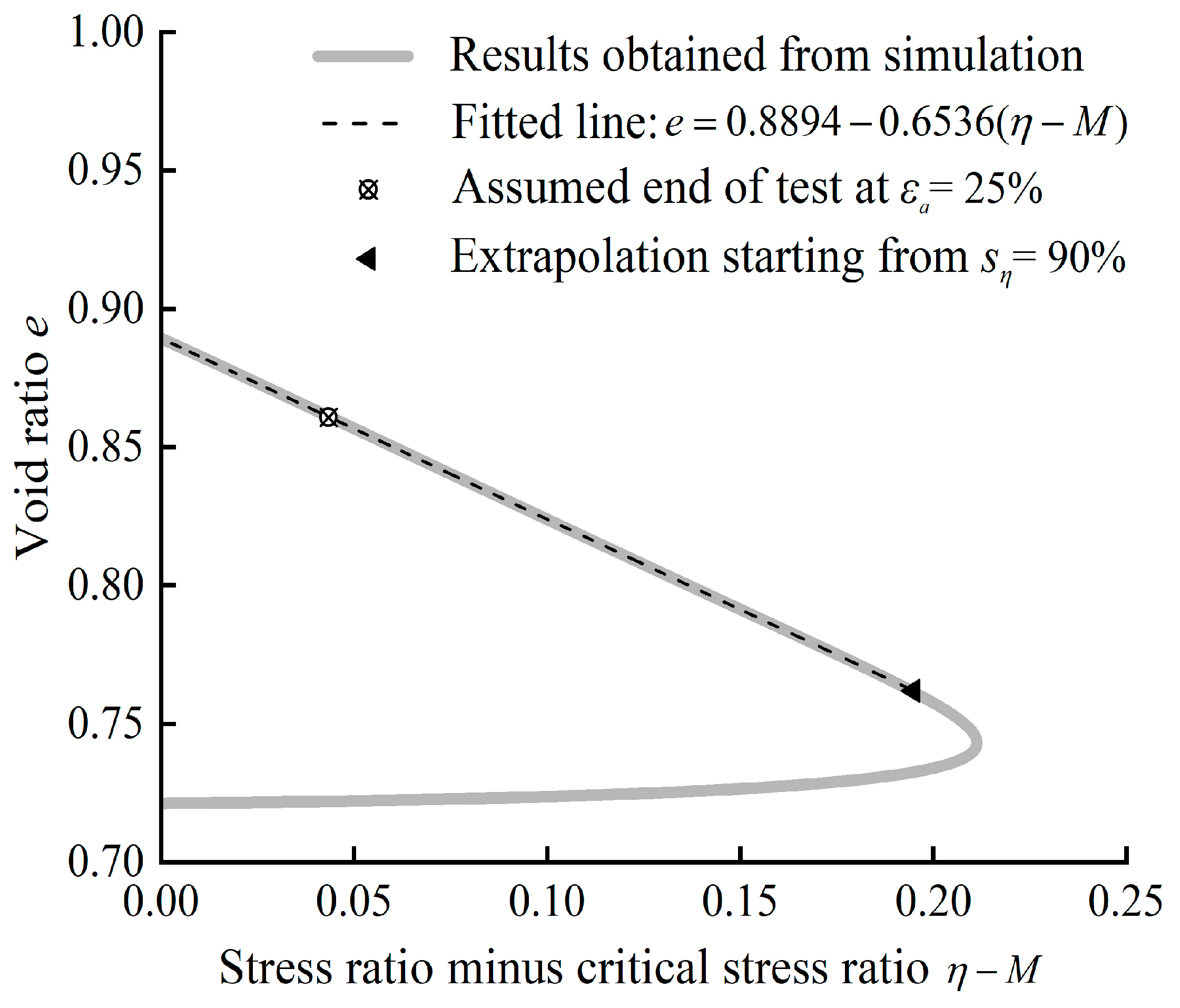
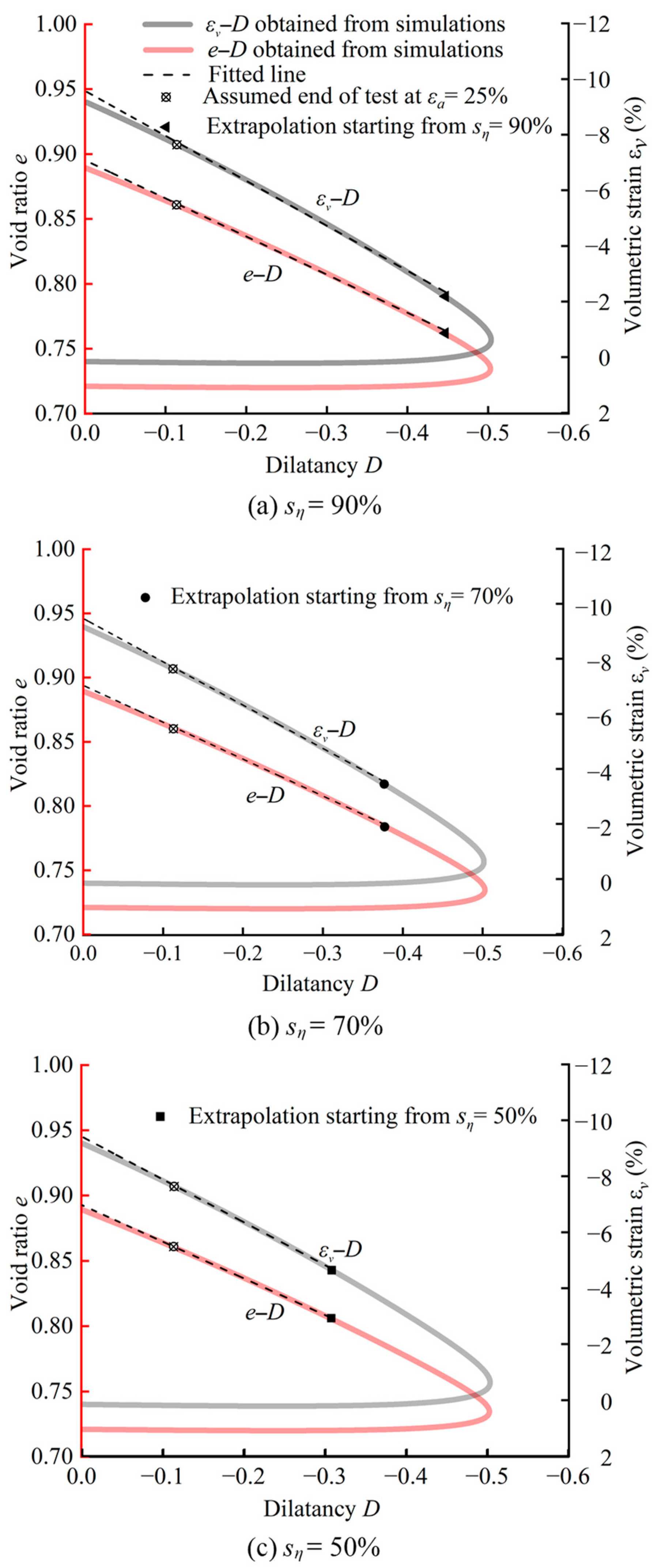
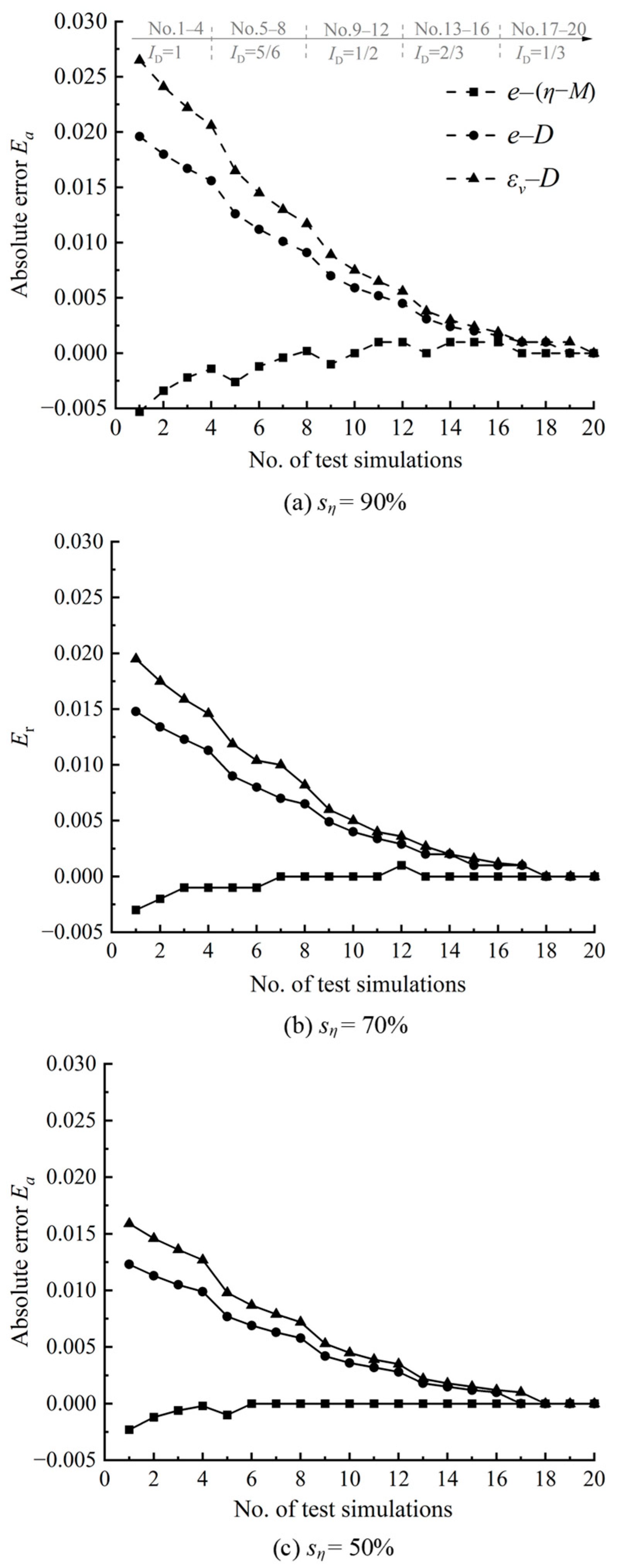
- During the strain-softening or dilating stage, the linearity between the e and η data is better than that between the e or εv data and D data. The e–η data are best suited to estimate the critical state void ratio with linear extrapolation.
- (b)
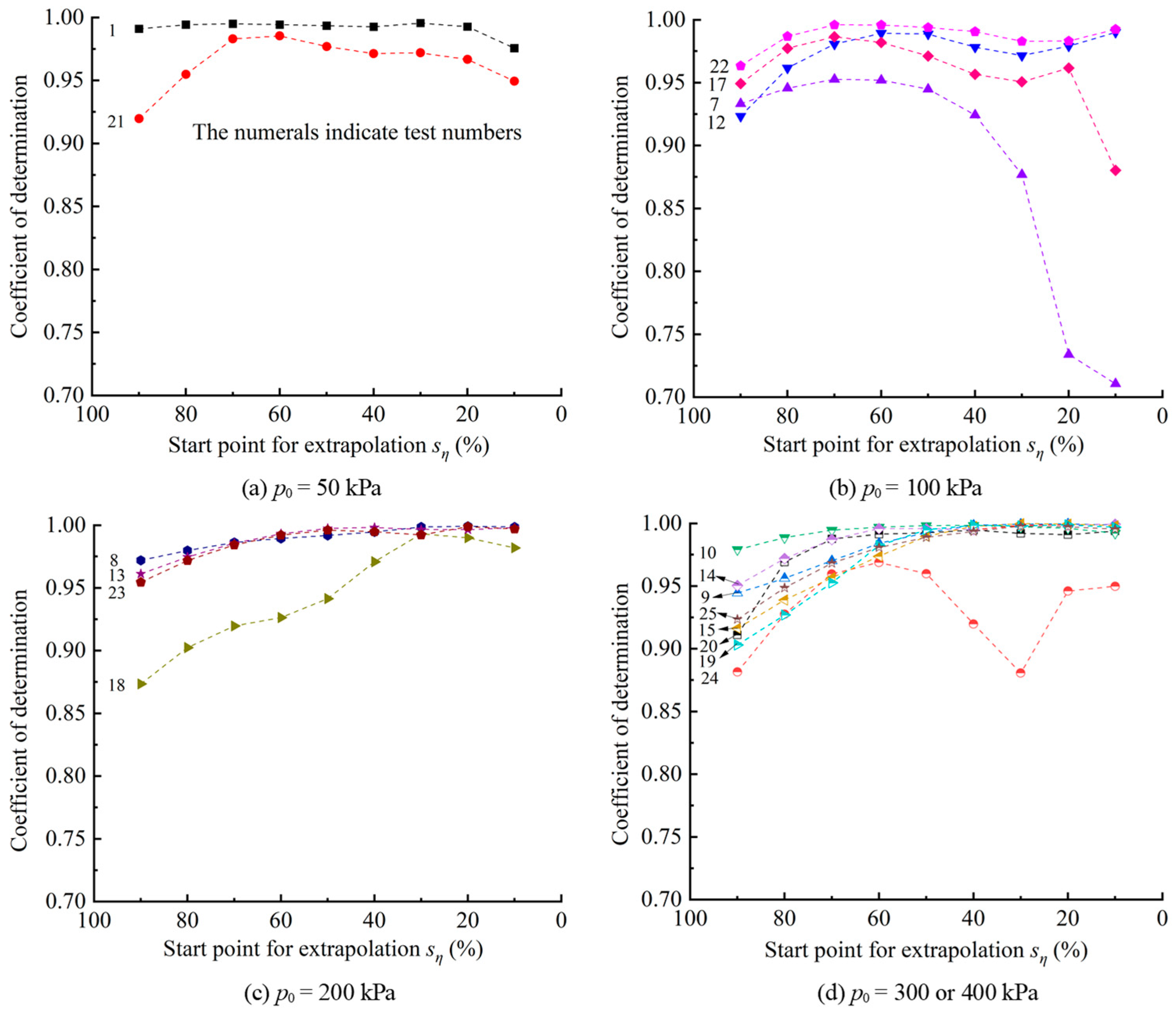
- The start point for fitting and extrapolating the e–η data has a significant influence on the accuracy of extrapolation. The greater the amount of the data used for fitting and extrapolation, the lower the extrapolation accuracy is.
- (c)
- Based on the experimental data considered, it is suggested to use the latter fifty percent of the post-peak e–η data to estimate the critical state void ratio with the linear extrapolation method.
- (d)
- Moreover, the e–η extrapolation method can be reasonably extended to other geotechnical materials whose strength and deformation characteristics can be captured by a state-dependent constitutive model (rubber–sand mixtures, silty sands, and rockfill materials). However, the recommendation of using the latter 50% of the post-peak data for extrapolation needs to be verified by further experimental study for extension.
Author Contributions
H.Z. proposed the method, analyzed the data, and plotted the figures. G.L. validated the results and wrote the original manuscript. All authors reviewed the manuscript. All authors have read and agreed to the published version of the manuscript.
Funding
This research was funded by the National Natural Science Foundation of China (grant number 51578213).
Institutional Review Board Statement
Not applicable.
Informed Consent Statement
Not applicable.
Data Availability Statement
The raw data supporting the conclusions of this article will be made available by the authors on request.
Conflicts of Interest
The authors declare no conflicts of interest.
Abbreviations
| CSL | critical state line |
| D | dilatancy (dilation rate) |
| D0 | dilatancy parameter |
| Dmin | minimum dilation rate |
| e | void ratio |
| e0 | intial void ratio |
| ecs | critical void ratio |
| ecses | estimated critical state void ratio |
| emin | minimum void ratio |
| emax | maximum void ratio |
| eΓ | critical state line parameter |
| Ea | absolute error |
| G | shear modulus |
| G0 | shear modulus parameter |
| h1 | plastic modulus parameter |
| h2 | plastic modulus parameter |
| K | elastic bulk modulus |
| Kp | plastic modulus |
| ID | density index |
| m | dilatancy parameter |
| M | critical stress ratio |
| n | hardening parameter |
| p | mean effective stress |
| p0 | initial (‘pre-shearing’) confining pressures |
| pa | atmospheric pressure |
| pcs | critical state mean effective stress |
| q | deviatoric stress |
| qcs | critical state deviatoric stress |
| sη | start point for extrapolation |
| η | stress ratio |
| ηEOT | stress ratio at the end of the test |
| φcs | critical state friction angle |
| ν | Poisson’s ratio |
| εa | axial strian |
| εq | deviatoric strain |
| plastic deviatoric strain | |
| εv | volumetric strain |
| plastic volumetric strain | |
| εvcs | critical state volumetric strain |
| ψ | state parameter |
| λc | critical state line parameter |
| ξ | critical state line parameter |
References
- Roscoe, K.H.; Schofield, A.; Wroth, A.P. On the yielding of soils. Geotechnique 1958, 8, 22–53. [Google Scholar] [CrossRef]
- Schofield, A.N.; Wroth, P. Critical State Soil Mechanics; McGraw-Hill London: London, UK, 1968; Volume 310. [Google Scholar]
- Wood, D.M. Soil Behaviour and Critical State Soil Mechanics; Cambridge University Press: Cambridge, UK, 1990. [Google Scholar]
- Been, K.; Jefferies, M.G.; Hachey, J. The critical state of sands. Geotechnique 1991, 41, 365–381. [Google Scholar] [CrossRef]
- Poorooshasb, H.B. Description of flow of sand using state parameters. Comput. Geotech. 1989, 8, 195–218. [Google Scholar] [CrossRef]
- Masín, D. Hypoplastic Cam-clay model. Geotechnique 2012, 62, 549–553. [Google Scholar] [CrossRef]
- Lu, Z.; Jin, Z.; Kotronis, P. Numerical analysis of slope collapse using SPH and the SIMSAND critical state model. J. Rock Mech. Geotech. Eng. 2022, 14, 169–179. [Google Scholar] [CrossRef]
- Cherif Taiba, A.; Mahmoudi, Y.; Azaiez, H.; Belkhatir, M. Impact of the overall regularity and related granulometric characteristics on the critical state soil mechanics of natural sands: A state-of-the-art review. Geomech. Geoeng. 2023, 18, 299–308. [Google Scholar] [CrossRef]
- Kaewhanam, N.; Chaimoon, K. A Simplified Silty Sand Model. Appl. Sci. 2023, 13, 8241. [Google Scholar] [CrossRef]
- Jagodnik, V.; Kraus, I.; Ivanda, S.; Arbanas, Z. Behaviour of Uniform Drava River Sand in Drained Condition-A Critical State Approach. Appl. Sci. 2020, 10, 5733. [Google Scholar] [CrossRef]
- Zhu, Z.; Cheng, W. Parameter Evaluation of Exponential-Form Critical State Line of a State-Dependent Sand Constitutive Model. Appl. Sci. 2020, 10, 328. [Google Scholar] [CrossRef]
- Novello, E.; Johnston, L. Geotechnical materials and the critical state. Geotechnique 1995, 45, 223–235. [Google Scholar] [CrossRef]
- Yu, H.S.; Zhuang, P.Z.; Mo, P.Q. A unified critical state model for geomaterials with an application to tunnelling. J. Rock Mech. Geotech. Eng. 2019, 11, 464–480. [Google Scholar] [CrossRef]
- Qi, Y.J.; Indraratna, B.; Vinod, J.S. Behavior of Steel Furnace Slag, Coal Wash, and Rubber Crumb Mixtures with Special Relevance to Stress-Dilatancy Relation. J. Mater. Civ. Eng. 2018, 30, 04018276. [Google Scholar] [CrossRef]
- Zhang, J.Q.; Wang, X.; Yin, Z.Y. DEM-based study on the mechanical behaviors of sand-rubber mixture in critical state. Constr. Build. Mater. 2023, 370, 130603. [Google Scholar] [CrossRef]
- Consoli, N.C.; de Azambuja Carvalho, J.V.; Wagner, A.C.; Scheuermann Filho, H.C.; Carvalho, I.; Cacciari, P.P.; de Sousa Silva, J.P. Determination of critical state line (CSL) for silty-sandy iron ore tailings subjected to low-high confining pressures. J. Rock Mech. Geotech. Eng. 2023. [Google Scholar] [CrossRef]
- Carraro, J.A.H.; Prezzi, M.; Salgado, R. Shear Strength and Stiffness of Sands Containing Plastic or Nonplastic Fines. J. Geotech. Geoenviron. Eng. 2009, 135, 1167–1178. [Google Scholar] [CrossRef]
- Xiao, Y.; Liu, H.; Ding, X.; Chen, Y.; Jiang, J.; Zhang, W. Influence of particle breakage on critical state line of rockfill material. Int. J. Geomech. 2016, 16, 04015031. [Google Scholar] [CrossRef]
- Azeiteiro, R.J.N.; Coelho, P.; Taborda, D.M.G.; Grazina, J.C.D. Critical State-Based Interpretation of the Monotonic Behavior of Hostun Sand. J. Geotech. Geoenviron. Eng. 2017, 143, 04017004. [Google Scholar] [CrossRef]
- Reid, D.; Fourie, A.; Ayala, J.L.; Dickinson, S.; Ochoa-Cornejo, F.; Fanni, R.; Garfias, J.; Da Fonseca, A.V.; Ghafghazi, M.; Ovalle, C.; et al. Results of a critical state line testing round robin programme. Geotechnique 2021, 71, 616–630. [Google Scholar] [CrossRef]
- da Fonseca, A.V.; Cordeiro, D.; Molina-Gómez, F. Recommended procedures to assess critical state locus from triaxial tests in cohesionless remoulded samples. Geotechnics 2021, 1, 95–127. [Google Scholar] [CrossRef]
- Mozaffari, M.; Liu, W.; Ghafghazi, M. Influence of specimen nonuniformity and end restraint conditions on drained triaxial compression test results in sand. Can. Geotech. J. 2022, 59, 1414–1426. [Google Scholar] [CrossRef]
- Indraratna, B.; Nimbalkar, S.; Coop, M.; Sloan, S.W. A constitutive model for coal-fouled ballast capturing the effects of particle degradation. Comput. Geotech. 2014, 61, 96–107. [Google Scholar] [CrossRef]
- Zhang, J.J.; Lo, S.C.R.; Rahman, M.M.; Yan, J. Characterizing Monotonic Behavior of Pond Ash within Critical State Approach. J. Geotech. Geoenvironmental Eng. 2018, 144, 04017100. [Google Scholar] [CrossRef]
- Li, W.; Coop, M.R. Mechanical behaviour of Panzhihua iron tailings. Can. Geotech. J. 2019, 56, 420–435. [Google Scholar] [CrossRef]
- Fotovvat, A.; Sadrekarimi, A.; Etezad, M. Instability of gold mine tailings subjected to undrained and drained unloading stress paths. Geotechnique 2022. [Google Scholar] [CrossRef]
- Yilmaz, Y.; Deng, Y.B.; Chang, C.S.; Gokce, A. Strength-dilatancy and critical state behaviours of binary mixtures of graded sands influenced by particle size ratio and fines content. Geotechnique 2023, 73, 202–217. [Google Scholar] [CrossRef]
- Zhang, J.; Lo, S.; Rahman, M.; Yan, J. Monotonic Behavior of Pond Ash under Critical State Soil Mechanics Framework. In Proceedings of the Geo-Congress 2014: Geo-characterization and Modeling for Sustainability, Atlanta, GA, USA, 23–26 February 2014; pp. 352–361. [Google Scholar]
- Torres-Cruz, L.A.; Santamarina, J.C. The critical state line of nonplastic tailings. Can. Geotech. J. 2020, 57, 1508–1517. [Google Scholar] [CrossRef]
- Ahmed, S.S.; Martinez, A. Triaxial compression behavior of 3D printed and natural sands. Granul. Matter 2021, 23, 82. [Google Scholar] [CrossRef]
- Velten, R.Z.; Consoli, N.C.; Scheuermann, H.C.; Wagner, A.C.; Schnaid, F.; Da Costa, J.P.R. Influence of grading and fabric arising from the initial compaction on the geomechanical characterisation of compacted copper tailings. Geotechnique 2022. [Google Scholar] [CrossRef]
- Li, X.S.; Dafalias, Y.F. Dilatancy for cohesionless soils. Géotechnique 2000, 50, 449–460. [Google Scholar] [CrossRef]
- Wichtmann, T. Karlsruhe Fine Sand Database. Available online: https://www.torsten-wichtmann.de/ (accessed on 1 September 2023).
- Li, X.S.; Wang, Y. Linear representation of steady-state line for sand. J. Geotech. Geoenviron. Eng. 1998, 124, 1215–1217. [Google Scholar] [CrossRef]
- Richart, F.E.; Hall, J.R.; Woods, R.D. Vibrations of Soils and Foundations; Prentice-Hall: Englewood Cliffs, NJ, USA, 1970. [Google Scholar]
- Verdugo, R.; Ishihara, K. The steady state of sandy soils. Soils Found. 1996, 36, 81–91. [Google Scholar] [CrossRef] [PubMed]
- Wichtmann, T.; Triantafyllidis, T. An experimental database for the development, calibration and verification of constitutive models for sand with focus to cyclic loading: Part I-tests with monotonic loading and stress cycles. Acta Geotech. 2016, 11, 739–761. [Google Scholar] [CrossRef]
- Youwai, S.; Bergado, D.T. Strength and deformation characteristics of shredded rubber tire sand mixtures. Can. Geotech. J. 2003, 40, 254–264. [Google Scholar] [CrossRef]
- Lashkari, A. Unified constitutive modeling of liquefaction in binary granular soils. In Proceedings of the 20th Annual International Conference on Mechanical Engineering–ISME2012, Shiraz, Iran, 16–18 May 2012. [Google Scholar]
- Xiao, Y.; Liu, H.; Chen, Y.; Jiang, J.; Zhang, W. State-dependent constitutive model for rockfill materials. Int. J. Geomech. 2015, 15, 04014075. [Google Scholar] [CrossRef]
- Liu, M.; Carter, J. A structured Cam Clay model. Can. Geotech. J. 2002, 39, 1313–1332. [Google Scholar] [CrossRef]
Disclaimer/Publisher’s Note: The statements, opinions and data contained in all publications are solely those of the individual author(s) and contributor(s) and not of MDPI and/or the editor(s). MDPI and/or the editor(s) disclaim responsibility for any injury to people or property resulting from any ideas, methods, instructions or products referred to in the content. |
© 2024 by the authors. Licensee MDPI, Basel, Switzerland. This article is an open access article distributed under the terms and conditions of the Creative Commons Attribution (CC BY) license (https://creativecommons.org/licenses/by/4.0/).