Abstract
In this paper, we propose the Soft Generative Adversarial Network (SoftGAN), a strategy that utilizes a dynamic borderline softening mechanism to train Generative Adversarial Networks. This mechanism aims to solve the mode collapse problem and enhance the training stability of the generated outputs. Within the SoftGAN, the objective of the discriminator is to learn a fuzzy concept of real data with a soft borderline between real and generated data. This objective is achieved by balancing the principles of maximum concept coverage and maximum expected entropy of fuzzy concepts. During the early training stage of the SoftGAN, the principle of maximum expected entropy of fuzzy concepts guides the learning process due to the significant divergence between the generated and real data. However, in the final stage of training, the principle of maximum concept coverage dominates as the divergence between the two distributions decreases. The dynamic borderline softening mechanism of the SoftGAN can be likened to a student (the generator) striving to create realistic images, with the tutor (the discriminator) dynamically guiding the student towards the right direction and motivating effective learning. The tutor gives appropriate encouragement or requirements according to abilities of the student at different stages, so as to promote the student to improve themselves better. Our approach offers both theoretical and practical benefits for improving GAN training. We empirically demonstrate the superiority of our SoftGAN approach in addressing mode collapse issues and generating high-quality outputs compared to existing approaches.
1. Introduction
With the rapid advance in deep learning techniques and access to vast amounts of data, generative models have come a long way in recent years. Generative Adversarial Networks (GANs) [1,2,3] belong to a powerful subclass of generative models. They work by pitting two networks against each other in a game-like scenario. The generator network creates synthetic data from a noise source, while the discriminator network distinguishes between the generator’s output and real data. Notably, these models can produce visually stunning outputs without explicitly computing the probability densities of the underlying distribution. Due to their ability to learn representations, GANs have been utilized in various fields, including data synthesis [4,5], semantic image editing [6], style transfer [7], image super-resolution [8] and classification [9]. However, achieving consistent and stable GAN training remains an ongoing challenge. Despite this, GANs often encounter another issue of mode collapse. This means that they tend to generate samples with limited diversity, even if they are trained on a dataset that is quite varied.
In this paper, we demonstrate specific strategies to stabilize GAN training, which lead to higher-quality image generation and potentially mitigate the mode collapse issue. In Section 4, we introduce the SoftGAN, a novel approach inspired by fuzzy set theory [10] and fuzzy concept modeling [11]. Our goal for the discriminator is to establish fuzzy concepts of real data, where the boundary between real and generated data is as soft as possible. To achieve this, we balance the principles of maximum concept coverage and the principle of maximum expected entropy of fuzzy concepts, as proposed in [12]. During the early stage of SoftGAN training, the principle of maximum expected entropy dominates the learning process due to the considerable divergence between the generated and real distributions. As the training proceeds, the principle of maximum concept coverage takes over, as the divergence between the two distributions diminishes. By constantly adjusting the discriminator’s tolerance based on the generator’s ability, we implicitly drive the generated distribution closer to that of real data while avoiding the issue of gradient vanish. In total, our contributions to the GAN-based generative models field are three-fold:
- Mitigating mode collapse and enhancing training stability through the dynamic borderline softening mechanism.
- Proposing a novel perspective of GAN training through the learning of fuzzy concepts. The discriminator aims to learn a fuzzy concept of real data with a soft borderline between real and generated data, achieving a balance between maximum concept coverage and the maximum expected entropy of fuzzy concepts.
- Offering theoretical and practical advancements in GAN training. Empirical evidence showcases the superiority of the SoftGAN in addressing mode collapse and generating higher-quality outputs compared to existing approaches.
The presented approach possesses numerous advantages when compared to state-of-the-art GAN-based generative models, as outlined below:
- The incorporation of the dynamic boundary softening mechanism enhances training stability and directs the generator to navigate through the entire training process without becoming ensnared in partial modes. The effectiveness of the SoftGAN in addressing mode collapse issues becomes evident through the examination of the Geometry Score indicator [13], as discussed in Section 6.3.
- Unlike WGAN-based methods [3,14,15,16] that focus on finding a discriminator that satisfies Lipschitz constraints to mitigate gradient vanishing, the SoftGAN adjusts the discriminator smoothness using the dynamic boundary softening mechanism. This prevents gradient vanishing while maintaining the convergence speed. Simultaneously averting gradient vanishing and sustaining the convergence speed, this mechanism ensures a balanced optimization process.
- The SoftGAN remains orthogonal to existing architectural techniques and regularization methods in GANs, allowing the effortless integration of our dynamic borderline softening mechanism into various GAN network architectures.
- Leveraging the approximated Earth Mover’s Distance between real and generated data distributions as an indicator, our mechanism effectively guides the parameter optimization direction during the generation process.
The rest of this paper is organized as follows. We first recall all notations, mathematical symbols and basic concepts in Section 2. Then, in Section 3, we present a review of the related works. The proposed idea is presented in Section 4 and Section 5 on the detailed method description and theoretical analysis, respectively. Then, the extensive experiments are provided in Section 6, followed by the conclusion in Section 7.
2. Preliminaries
Generative Adversarial Networks: As a generative model, Generative Adversarial Networks (GANs) achieve the implicitly statistical distribution capture of training data through game training. A common analogy used to explain their mechanism is to think of one network as an art forger (generator G) and the other as an art expert (discriminator D). G creates forgeries with the aim of producing realistic images, while D receives both forgeries and real images and aims to distinguish between them. Both networks are trained simultaneously and in competition with each other [17]. This two-player minimax game is formalized mathematically as follows:
where is the prior distribution from which input samples z to the generator are drawn (usually standard Gaussian) and represents the target distribution associated with the training data. represents the expected value with respect to the distribution specified in the subscript.
In the training stage, GANs always follow an alternating fashion by minimizing the adversarial loss as the object of the discriminator and generator, respectively:
Fuzzy Concept Modeling: Fuzzy concept modeling has fundamental importance in Cognitive Psychology and Artificial Intelligence. One prominent work on this topic is prototype theory [11]. The fundamental idea of prototype theory is that concepts are represented by a set of prototypical cases P. These cases correspond to those elements of the underlying conceptual (attribute) space that are certain to satisfy the concept. Meanwhile, the fuzzy concept L has the form “about P”, “similar to P” or “close to P”, and “about”, “similar to” and “close to” are fuzzy constraints. Hence, For any element , we can measure the membership degree that it belongs to the fuzzy concept L.
For the convenience of understanding, we summarized all the notations for the preliminaries and our approach as a quick list in Table 1.

Table 1.
Notations quick list.
3. Related Works
As described in Section 2, the training mechanism of GANs based on game theory is elegant, but it is known to be unstable during training and may not converge at all. Therefore, one must seize the best opportunity of alternate iterations of G and D, carefully grasping the balance between the two. In addition, another common issue with GANs is that they often produce samples with limited diversity, even when trained on a diverse dataset. Specifically, when the generator G finds out that one or several generated outputs can easily deceive the discriminator D, it might limit itself to only generating those samples without exploring other possibilities. This phenomenon is known as mode collapse.
While training instability is a critical factor in mode collapse, there is currently no known method in the literature that addresses both issues simultaneously to improve GAN training. There are a series of WGAN-based works [3,14,16,18] that claim to solve the problem of training instability, which can help reduce mode dropping. However, there has been no detailed discussion or explanation of why mode collapse is reduced in these methods. Additionally, these methods face difficulties in effectively meeting Lipschitz continuity and require complex network architectures (such as the ResNet block [19], Style block [20,21,22] and Skip block [23]) to achieve optimal results. Furthermore, as noted in [14], these approaches have a slower convergence speed compared to the original version [1,2].
In addition to the above-mentioned training instability and mode collapse problems, the theoretical studies on GANs are generally divided into three directions: the improvement of the objective function, the introduction of training techniques and the proposal of an evaluation indicator. The research in this paper belongs to the first direction. In this direction, the most successful research is a series of WGAN-based studies, as far as we know [3,14,16,18]. Among them, the most relevant to ours is WGAN-C [15]. The authors, Sharma et al. [15], also use the analogy of teaching and learning to describe the whole training process. The SoftGAN adjusts the tolerability of the discriminator to the generator through the dynamic borderline softening mechanism from the perspective of fuzzy concept learning, while WGAN-C draw lessons from the progressive idea based on WGAN-GP [14] to control the discriminant ability with a set of convex combinations of predefined multiple discriminators. Although both use the analogy to learning, they are different in their implementation and motivation. In addition to the above methods, there are some approaches that reduce the risk of falling into local modes by building multiple discriminators or multiple generators, such as Dropout-GAN [24], D2GAN [25], GMAN [26] and DuelGAN [27]. These methods can significantly improve the robustness of the model through the collaboration of multiple discriminators or generators, but they exponentially increase the size and training difficulty. In contrast, the training cost of our SoftGAN is much lower.
4. SoftGAN
In this section, we propose the SoftGAN, which solves the training instability and mode collapse problem of the GAN simultaneously. It is a new discriminator mechanism that can dynamically adjust the tolerance of the discriminator to samples. We will explain the details of our approach below.
The training failure in the original GAN can be attributed to the discriminator completely differentiating between real and generated samples. It creates a hard boundary (or cliff) between the discriminant outcomes, preventing the generator from receiving practicable gradients and impeding its improvement, as depicted in Figure 1. Building upon this observation, we introduce a novel training objective for the discriminator. In our SoftGAN, the discriminator aims to implicitly learn a fuzzy concept of samples from distribution. And the output of the discriminator for each real/generated sample is the degree of membership of the sample to the fuzzy concept. During the early stages of training, the boundary of the fuzzy concept is uncertain. So, the discriminator will not completely negate the generator to lead to the problem of gradient vanishing. As the training progresses, the boundary of the fuzzy concept shrinks and the uncertainty decreases. Correspondingly, the ability of the discriminator increases with the decrease in uncertainty, and the generated distribution learned by the generator gradually approaches the distribution of real data.
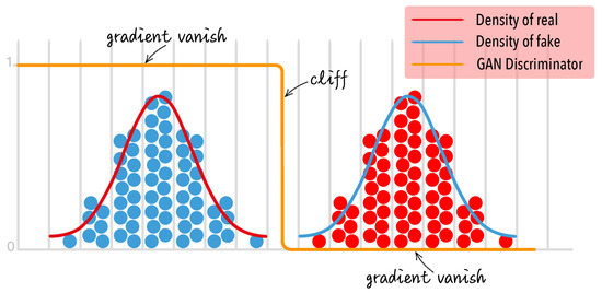
Figure 1.
The discriminator of the original GAN is responsible for distinguishing between two distributions. At the beginning of training, there exists a distinct boundary (or cliff) between the discriminant outcomes, which prevents the generator from receiving the gradient information it needs to enhance its performance.
Formally speaking, the discriminator tries to learn a fuzzy concept D and its negation to describe real samples from and fake samples from , respectively. And the borderline between D and should be as soft as possible.
In the following, we use to represent the degree of sample x belonging to the fuzzy concept D. In other words, represents the degree of the concept coverage of D to the sample x. Then, the entropy
reflects the degree of sample x being a borderline case between D and , where . We name this entropy fuzzy entropy of D. In particular, , which means that a fuzzy concept has the same uncertainty of borderline with its negation. According to the above definition, we have the following:
- reflects the concept coverage of D with respect to the true distribution .
- reflects the concept coverage of with respect to the generated distribution
- reflects the uncertainty of the borderline between D and with respect to distribution .
- reflects the uncertainty of the borderline between and D with respect to distribution .
According to the work by Tang and Xiao [12], when learning a fuzzy concept D from samples we should adopt two learning principles of maximum concept coverage and maximum fuzzy entropy:
where is a factor compromising the concept coverage and the fuzzy entropy. So, in order to learn a fuzzy concept D and its negation for distributions and , respectively, the discriminator D has the following two subobjective functions:
In total, for our proposed SoftGAN, the value function is defined as follows:
When incorporating both the goals of the discriminator D and the generator G, the minimax game between D and G is as follows:
The in Equation (4) is the weight of the fuzzy entropy term (we also can call it the encouragement term), which is used to control the uncertainty of the borderline between real samples and fake samples. The contribution of the to regulating the entropy is three-fold:
- In the early training stage, the larger can make a global search, which pushes the generated distribution to have multiple modes, since it forces the support set of to be the same as the support set of : (see the theoretical analysis in Proposition 3 of Section 5).
- In the early training stage, the larger can also be helpful to improve the tolerance of the discriminator, which will be effective to avoid gradient vanishing and to accelerate the training process.
- As the capability of the generator increases, the discriminator also becomes very rigorous. The smaller can make a local search, and the generator is forced to produce samples similar to the real ones, which means the generated quality will be enhanced.
In brief, we call this process the dynamic borderline softening mechanism.
To better illustrate the dynamic borderline softening mechanism, let us use the analogy of a tutor and a student instead of an art forger and an art expert. The generator, acting as the student, aspires to learn effectively, while the discriminator, acting as the tutor, aims to guide the student in the best possible way. Initially, the student struggles to grasp the key points and barely completes the task. At this stage, the tutor appropriately lowers the standards, allowing the student to pass exams. This approach provides the student with more encouragement and confidence, fostering improvement. As the student progresses, the tutor gradually raises the requirements to motivate the student to develop in a more advanced direction. Through continuous encouragement, the student steadily grows and meets the qualifications even as the standards improve. Ultimately, the student becomes capable of excelling even when faced with challenging problems.
Similarly, let us examine the issue of mode collapse from the perspectives of the tutor and the student. The reason behind the existence of mode collapse lies in the generator discovering that certain modes it generates receive high evaluations from the discriminator. Consequently, it tends to solely focus on generating those modes and avoids generating modes where its performance is lacking. This can be compared to a student who excessively focuses on or enjoys certain subjects while disliking others where they struggle to achieve good grades. In order to receive praise from their tutor, the student consistently works on improving their skills in subjects they excel at while avoiding the challenges posed by subjects they struggle in. This phenomenon results in them leaning towards their strengths rather than a balanced overall learning experience. To address this problem, the tutor should encourage the student to maintain a balanced approach to their studies. The tutor can achieve this by initially setting lower standards when the student does not display a clear preference towards any subject. Subsequently, the tutor can gradually raise the requirements in a balanced manner to motivate the student towards overall progress.
We can also reconsider the dynamic borderline softening mechanism from an optimization viewpoint. The weighted fuzzy entropy term (encouragement term) can be seen as a penalty term that helps in smoothing the curve of the objective function. By smoothing the curve, we can bypass local optimal solutions and approach the vicinity of the global optimal solution. As the value of decreases, the degree of curve smoothing decreases, eventually approximating the actual objective function curve. At this point, the local optimal solution obtained through gradient descent is equivalent to the global optimal solution.
To achieve the desired dynamic control mentioned above, it is important to consider the weight factor, represented as , in relation to the disparity between the distributions of generated data and real data. To measure this correlation, we introduce the Earth Mover’s Distance [28]. During the training process, after several iterations, an equal number of samples are randomly selected from both the generated data and the real data. The Earth Mover’s Distance between the two distributions is then calculated. The updated value of is determined by scaling the Earth Mover’s Distance between these two distributions. In the experimental section, we scale the Earth Mover’s Distance to fit within the range of . Then, we clamp it by the upper bound to update . The proof of the upper bound of is in Proposition 4.
So far, we have provided a detailed explanation of the proposed method, and we summarize it in Algorithm 1. Regarding the optimization algorithm choice, we uniformly utilize the Adam algorithm [29]. Additionally, we employ a clever strategy to expedite the training process for updating G. When it comes to the minimization problem
it shares the same solution as
However, Equation (6) is more susceptible to being trapped in a local minimum compared to the latter. Therefore, in Algorithm 1 (line 9), we directly calculate Equation (7) to achieve the same objective.
| Algorithm 1: Framework of SoftGAN |
 |
Fundamentally, the original GAN also can be interpreted from the perspective of fuzzy concept learning, much like the SoftGAN. The goal of the discriminator in the original GAN is also to learn a fuzzy concept, D, that models the true distribution, as depicted in Equation (1). In comparison to the SoftGAN, the learning principle of the original GAN only aims to maximize the concept coverage. This ensures that the learned fuzzy concept, D, and its negation, , fully encompass the real and generated data, respectively. Simultaneously, the objective of generator is to produce samples that fall within the purview of the fuzzy concept D, thereby leading the discriminator to misidentify them as real data. Directed by this single learning principle, the fuzzy concept can discern the real data from the generated data in a quite “hard” manner. In contrast to the original GAN, the SoftGAN introduces a new learning principle: the principle of maximum expected entropy. This ensures that real and generated data are merely the borderline cases of the fuzzy concepts D and , respectively. In simpler terms, the SoftGAN discriminates between real and generated data in a “soft” way.
5. Theoretical Analyses
In this section, we present a comprehensive theoretical analysis of the optimality within the minimax game of the SoftGAN. Alongside this, we provide an interval analysis for the hyperparameter , which is the kernel to the dynamic borderline softening mechanism.
5.1. Optimality of the Discriminator
Proposition 1.
For a given generator G, the optimal discriminator D is as follows:
where is the sigmoid function.
Proof.
According to Equations (4) and (5), for a given generator G, the training criterion for the discriminator D is to maximize the following value function marked as J:
Let F be the following form:
Then, . Combined with Equation (3) and , the first and second derivatives of F with respect to are as follows:
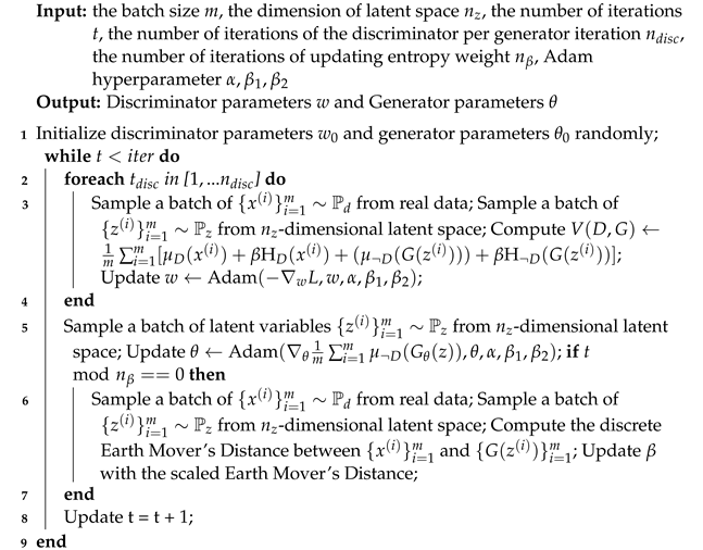
Next, we analyze the discriminator D qualitatively. According to Equation (8), when and . For the interval where , the value of , which is negatively correlated with the Earth Mover’s Distance between and . The larger the distance is, the smaller the is, and the smaller the distance is, the larger the is. As the training progresses, moves in the direction of , and the Earth Mover’s Distance between the two distributions decreases gradually. Correspondingly, the curve of the also becomes flatter and flatter. When the training is over, in the entire domain. The schematic diagram of this process is shown in Figure 2.
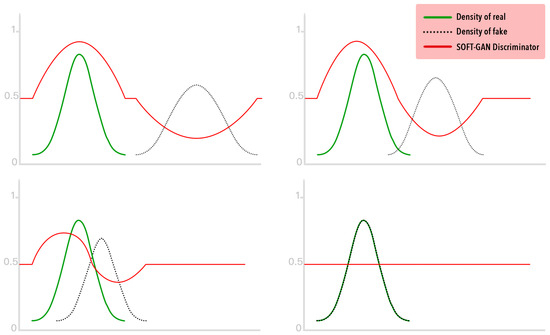
Figure 2.
The schematic diagram of the training process for SoftGAN. The y-axis represents .
5.2. Optimality of the Generator
Now, let us focus on the optimal generator G. We discuss this issue in both and cases.
Proposition 2.
When and for any x, the global optimum of Equation (5) is achieved if and only if almost everywhere.
Proof.
Let , and . According to Equation (8), we have
When given and , the training criterion for the generator G is to minimize the following function Q according to Equation (5):
Then, using the trick of adding and subtracting the same object, we obtain the following:
Consequently, Q reaches the minimum value if and only if almost everywhere. □
Proposition 3.
When , the algorithm will force the support set of to approximate to the support set of : .
Proof.
For the training of , according to our optimizing trick as shown in Equation (7), we have the following:
According to Equation (8), we have the following:
Thus, we have the following form:
When , we have . So, in order to maximize the lower bound, we have either for or . In other words, when , for any , either or .
In addition, we also need to avoid the situation for the goal of the generator. In summary, we have the above Proposition 3. □
According to this proposition, we can conclude that in the SoftGAN not only makes a global search of distribution comprehensively but also assigns the non-zero density of the generated distribution to the support set of the true distribution. This kind of open-minded strategy naturally avoids the mode collapse problem. So, in the very early training stage, the generated distribution will have enough multiple modes.
5.3. Interval Analysis of
Proposition 4.
The upper bound of β is .
Proof.
There are two extreme cases for the relationship between and . One is that the discriminator completely separates the two, and their distributions are disjunct. The other is that the discriminator cannot tell the two apart, and their distributions are almost indistinguishable. Obviously, what we want is the second extreme case. Therefore, for the minimization optimization problem of , after the introduction of , it is necessary to ensure that the extreme value obtained in the second case is smaller than the first case:
When and do not intersect, the discriminator completely separates the two:
When and are almost the same, the discriminator cannot separate them at all:
In order to ensure that the minimized optimization problem achieves the desired solution, there must be
So, . □
Finally, we give an intuitive explanation of the hyperparameter . According to Proposition 1, the optimal discriminator is a sigmoid function about and with the control of . The relationship between and discriminator D is shown in Figure 3. As mentioned before, is used to control the tolerability of the discriminator. The larger is, the more uncertain the soft borderline is and the higher the tolerance of the discriminator is, and vice versa.
Figure 3.
The influence of different values to the discriminator D. is proportional to the uncertainty of the soft borderline.
6. Experiments
In the following section, we will showcase the practical benefits of our method while providing an in-depth comparison between its behavior and that of traditional GANs. Specifically, this part consists of five subsections:
- (1)
- We conducted a series of controlled experiments on two real-world datasets [30,31]. On the one hand, we verified the effectiveness of the dynamic borderline softening mechanism proposed in Section 4. On the other hand, we demonstrated the qualitative and quantitative superiority of the SoftGAN compared to other algorithms [2,14,18,23,32,33,34,35,36,37,38,39] under the same architecture configurations.
- (2)
- The learning goal of the generative model is to implicitly approximate the distribution of the real data. We used qualitative and quantitative methods to visualize the distribution distance change between real data and generated data during training. It verified the effectiveness of the dynamic borderline softening mechanism of our SoftGAN.
- (3)
- The mode collapse in GAN training is one of the research focuses of the SoftGAN. With the help of the Geometry Score [13], we quantitatively compare the mode coverage ability and the mode discovery efficiency of our SoftGAN with other methods [2,14] in the training process.
- (4)
- Evaluating the mode coverage of a generative model on datasets with limited categories poses challenges. However, on datasets containing numerous categories, a generative model boasting robust mode coverage capabilities is expected to generate samples from a broader range of categories. As a result, we employed a classifier model [40] to assess, specifically on the ImageNet dataset [41], whether our model’s generator exhibits enhanced coverage across all 1000 categories. This evaluation indirectly serves as evidence of the SoftGAN’s mode exploration prowess.
- (5)
- Our work introduces a flexible dynamic borderline softening mechanism, which seamlessly integrates into pre-existing GAN frameworks. By combining this mechanism with diverse architectures [1,19,20,42] and varied adversarial losses [1,3,14,20,23], we have successfully demonstrated that the SoftGAN can enhance the target model’s capabilities without compromising the quality of the generated outputs, as evidenced by qualitative and quantitative indicators. Additionally, the parameter sharing approach for shallow layers effectively alleviates computational burdens, further enhancing the efficiency of the model.
All experiments are conducted on four Nvidia GeForce RTX 3090 graphics cards with 24 GB implemented in Pytorch [43]. For the hyperparameter , we use its theoretical upper bound (as shown in Proposition 4) as the initial value in all experiments. And the demo implementation is available at Github (https://github.com/liweileev/SoftGAN, accessed on 23 August 2023).
6.1. Quality of Generated Image under Basic Architectures
In this section, we conduct experiments on real-world large-scale datasets [30,31] and present both qualitative and quantitative evaluation results. To ensure a fair comparison, we adopt experimental settings that are identical to those used in previous works [14,18] under the same basic architecture configurations. As a result, we list the results from the unconditional unsupervised GAN-based models and compare them with our SoftGAN.
Similar to WGAN-GP [14] and CT-GAN [18], we utilize the CIFAR-10 [30] dataset to evaluate two architecture configurations for the generative model: one is a small CNN architecture, and the other is a ResNet architecture. Table 2 and Table 3 show the two architectures, respectively.
Table 2.
The small CNN architecture for SoftGAN on CIFAR-10 [30]. The traning batch size is 32.
Table 3.
The ResNet architecture for SoftGAN on CIFAR-10 [30]. The traning batch size is 32.
For quantitative comparison, we use the Inception Score [35] as the evaluation indicator, similar to CT-GAN [18], and the specific comparison results are shown in Table 4. As shown in the experimental results, the SoftGAN with the small CNN architecture is not bad, and the SoftGAN with ResNet surpasses all of the isomorphic unconditional GAN-based methods in the performance of the Inception Score. It is worth noting that some of the methods [36,37] in Table 4 also use the multi-discriminator or multi-generator tricks. Theoretically, under the same architectural configuration, the trick of parallel subnetworks can improve the generation capability of the model. However, the SoftGAN still has a significant performance advantage in comparison. Furthermore, these techniques are fully orthogonal to our study, and they can be used together to enhance the model performance. Experiments with combinations of different network architectures and training techniques are presented in Section 6.5. In addition, we found that the dependence of our approach on the network architecture (small CNN: 6.46 ± 0.42; ResNet: 8.55 ± 0.05) is significantly lower compared with other methods, such as WGAN-GP [14] (small CNN: 2.98 ± 0.11; ResNet: 7.86 ± 0.07) and CT-GAN [18] (small CNN: 5.12 ± 0.12; ResNet: 8.12 ± 0.12). Whether in a simple network architecture or a complex network architecture, our proposed method has strong robustness and generates samples with considerable Inception Scores.
Table 4.
Inception Scores of GAN-based models with the same architecture configurations on CIFAR-10 [30]. Here, ± refers to the standard deviation returned by the Inception Score calculator.
Figure 4 shows images generated by our models with their Inception Scores. The entire Inception Score curves during the training are shown in Figure 5, which demonstrates the superiority of our approach in image generation quality.
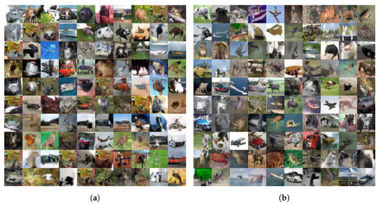
Figure 4.
Samples generated by SoftGAN and their Inception Scores on CIFAR-10 [30]: (a) samples generated by a small CNN SoftGAN and their Inception Score: 6.46 ± 0.42; (b) samples generated by ResNet SoftGAN and their Inception Score: 8.55 ± 0.05.
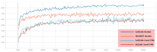
Figure 5.
Inception Scores of different models in CIFAR-10 dataset. The horizontal axis represents the number of iterations, and the vertical axis represents Inception Scores. The higher the score, the better the quality of the generated image.
We also trained the ResNet SoftGAN model on the LSUN bedroom dataset [31] which contains 3,033,041 images of bedroom. The generated samples are shown in Figure 6. Qualitatively speaking, it is also competitive with other methods for this dataset.
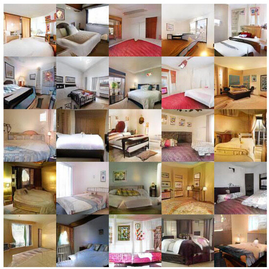
Figure 6.
Samples of size generated by SoftGAN ResNet model in LSUN bedroom dataset [31].
6.2. Divergence Evolution between Real and Generated Distributions
As mentioned before, we employ the Earth Mover’s Distance (EMD for short) to measure the divergence between the distributions of real data and generated data, as well as to quantify the value of after scaling. So, the value of the EMD is used as an indicator to check whether the updating direction of the generator is correct. It is also used to achieve the dynamic borderline softening mechanism proposed in this paper. In practice, the computation of the EMD is based on the batch sampling, so the approximated EMD does not converge to 0 due to the variance in the data (as shown in Figure 7). As the training progresses, the EMD between and decreases rapidly. This indicates that the principle of maximum expected entropy dominates the learning process and enables , as deduced in Proposition 3. Then, due to the adjustment of , the alters continuously within the support of and gradually approaches the real distribution. At this stage, the principle of maximum concept coverage dominates the learning process, so the EMD between and does not change much, but the quality of the generated samples is gradually improved.
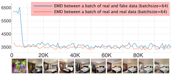
Figure 7.
The change in the Earth Mover’s Distance (EMD) during the training process with corresponding generated samples (LSUN bedroom dataset [31]). The horizontal axis represents the number of iterations of the training, and the vertical axis represents the Earth Mover’s Distance calculated using a batch of samples. The images below are the images generated from the same noise for every 10,000th iteration. The pictures are best viewed magnified on screen.
6.3. Mode Discovery and Mode Coverage
In this experiment, we would like to study how our approach behaves for the mode collapse problem. To achieve this, we train three GAN models: DCGAN [2], WGAN-GP [14] and our SoftGAN. We use the Geometry Score [13] to assess the mode discovery and mode coverage abilities of different models. This approach allows us to compare the topology of the underlying manifolds for point clouds in a stochastic manner, providing us with a visual way to detect the mode collapse and a score, which allows us to compare the quality of various trained models. The lower the score is, the more modes are covered by the generated images. If the value of the Geometry Score does not decrease or even rises as the training progresses, the model may suffer from the mode collapse problem. Following the parameter settings of the original works, we train each model for 100,000 iterations and generate 1000 samples every 100 iterations to evaluate the Geometry Score using the parameter . Since the Geometry Score is calculated with only 1000 samples, the results are fluctuating. So, we smooth the result using the tool in Tensorboard (a suite of visualization tools to make it easier to understand, debug and optimize the machine learning workflow) with the smoothing parameter equal to 0.6 and then report the obtained results in Figure 8. It can be seen from the figure that the SoftGAN shows an advantage in mode coverage at the beginning of training. Compared with those of WGAN-GP and DCGAN, the Geometry Score of our method rapidly decreases to a lower value and is almost at a relatively lower level compared to the other two.
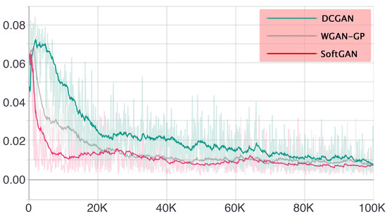
Figure 8.
Comparison of different methods with Geometry Score in the CIFAR-10 dataset [30]. The horizontal axis represents the number of training iterations, and the vertical axis represents the Geometry Scores of different models. Samples used to calculate scores are generated using DCGAN, WGAN-GP and SoftGAN. Mode collapse can be measured using the Geometry Score. The translucent curves are the results of the real calculation, because only 1000 samples are involved in the calculation, so the results are dithered, and the deep color curves are the smoothed result. The lower the score, the more diverse modes the generated images covered.
6.4. Category Coverage on Complex Dataset
To assess the mode coverage capability of a generative model for datasets containing a limited number of categories, we can examine the diversity of generated samples within each category. However, this qualitative observation makes it challenging to compare among different models. In the case of datasets with numerous categories, the problem becomes more straightforward. If a generative model asserts a stronger mode exploration capability, it should generate samples that encompass a broader range of categories compared to other models. And just a classifier is enough to qualitatively measure this distinction.
We opt to utilize ImageNet [41] as the benchmark dataset. ImageNet is an extensive collection of visual data, comprising 1,281,167 training images and 50,000 validation images across 1000 object classes. Over time, it has emerged as the go-to dataset to evaluate and compare image classification algorithms. The dataset’s substantial sample size and diverse range of categories present significant challenges for high-resolution (≥256) and unconditional image generation tasks. We select it as our benchmark for two key reasons:
- Its vast and varied categories suit our objective of measuring diversity.
- There exist readily available, pretrained classifiers that enable us to assess the category coverage of the generated samples.
For this experiment, we adopt StyleGAN2 [21,22] as our baseline model. The generator architecture consists of a mapping network, which comprises two fully connected layers, and a synthesis network that progressively expands from a resolution of to . In contrast, the discriminator employs a convolutional neural network with skip connections, progressively reducing the resolution from to . You can find more detailed network information and parameter quantities in Table 5. Except for the dynamic borderline softening mechanism in our SoftGAN, the remaining training parameters of StyleGAN2 and ours are identical, including the batch size (32) and the optimizer (Adam [29]), as well as the usage of style loss, path length regularization and lazy R1 regularization.
Table 5.
The architectural design of the generator and discriminator utilized in SoftGAN and StyleGAN2 for the ImageNet [41] generation task.
We completed 50 epochs training for both models. Subsequently, BEit [40] was employed to categorize a set of 50,000 generated samples for each of the two models. The outcomes of the classification endeavor have been depicted visually in Figure 9. To facilitate comparative analysis, we not only present the classification results of the generated outputs from StyleGAN2 and our SoftGAN but we also illustrate the labels and BEiT classification results of real data. This demonstration serves to underscore the efficacy of the employed classifier. Within each image, an assemblage of 1000 squares has been incorporated. These squares function as a representation of the comparative statistical occurrence of individual classes within the corpus of 50,000 samples. The squares colored in shades of blue denote the inclusion of the respective category, with darker hues indicating higher frequencies. Conversely, the presence of a red cross signifies the absence of the category. A noteworthy observation emerges when comparing the categories covered by the SoftGAN to those covered by StyleGAN2. Remarkably, the SoftGAN exhibits a noticeably superior coverage, surpassing even the performance of random sampling on real data. To provide a quantitative perspective, the StyleGAN2 encompasses 958 distinct ImageNet categories, with a shortfall of 42 categories. In stark contrast, the SoftGAN only misses 4 categories.
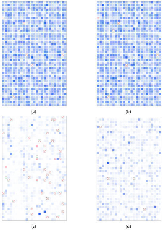
Figure 9.
Visualization of classification results for ImageNet dataset [41]. In each subfigure, 1000 squares are displayed, each representing one of the 1000 categories present in ImageNet. The coloration of these squares reflects the quantity of samples within each corresponding category, with darker shades indicating a higher sample count. Furthermore, any categories that are absent from the set are denoted by conspicuous red crosses. (a) Real labels of 50,000 images randomly sampled from the shuffled dataset. The category coverage is 99.4%, and the entropy is 6.89. (b) Classification results of BEiT [40] for same images in (a). The top-1 accuracy is 94.36%, and the top-5 accuracy is 99.55%. (c) Classification results for 50,000 StyleGAN2 generated images. The category coverage is 95.8%, and the entropy is 6.17. (d) Classification results for 50,000 SoftGAN-generated images. The category coverage is 99.6%, and the entropy is 6.69.
Additionally, we assess the quantitative metric pertaining to the category distribution within the real and generated samples:
where N represents the sample size of 50,000, C denotes the total number of categories (1000) and corresponds to the count of samples in the ith category. This approach evaluates the information entropy of the sample distribution, with larger values indicating greater diversity. Notably, for random sampling of real samples, the information entropy measures 6.89, suggesting a distribution close to uniform. In the case of generated samples, StyleGAN2 yields an information entropy of 6.17, while the SoftGAN registers an information entropy of 6.69. The comparison reveals that the SoftGAN generates samples with a broader coverage and increased diversity in comparison to StyleGAN2.
Moreover, it is pertinent to underscore that in contrast to the random sampling of real shuffled data, both StyleGAN2 and the SoftGAN exhibit non-uniformity in their randomly generated outputs. A discernible discrepancy arises in the intensity of square coloring across categories. Certain categories manifest a markedly darker hue, signifying a higher sample count, compared to others. Evidently, these findings indicate a lack of impartiality in the outputs of the generators, even in scenarios involving stochastic noisy inputs. Our conjecture is that this phenomenon could be intricately tied to the inherent sampling domain of the generator. The exploration of this intriguing matter, however, lies beyond the scope of the current study.
6.5. Architecture and Training Tricks in Combination with SoftGAN
The previous experiments have confirmed the benefits of the SoftGAN in terms of its ability to explore modes within both simple and complex datasets. Apart from the mode coverage, the quality of generated samples is also crucial in evaluating generative models. Consequently, this section aims to quantitatively compare the variation in generation quality between the SoftGAN and other GANs using three datasets: CIFAR-10 [30], STL-10 [45] and CelebA [46]. To assess the quality, we employ the widely recognized Fréchet Inception Distance [47] (FID) as the metric. The FID measures the dissimilarity between the distribution of generated images and the distribution of real images used for training. Unlike pixel-based comparisons, the FID evaluates the mean and standard deviation of the output from the intermediate layer of Inception v3 [48], which approximates the human perception of image similarity. Over the years, the FID has become the standard metric for evaluating GAN quality. As previously mentioned, our dynamic borderline softening mechanism is completely independent of other generator architectures and training techniques used in GANs. To demonstrate the versatility of our approach, we conducted experiments by integrating it into other models. Specifically, we compared GAN models using three different architecture combinations: linear generator + linear discriminator, ResNet generator + skip discriminator and style generator + linear discriminator. The network architectures of the various components are depicted in Figure 10, and the detailed FID comparison results are presented in Table 6.
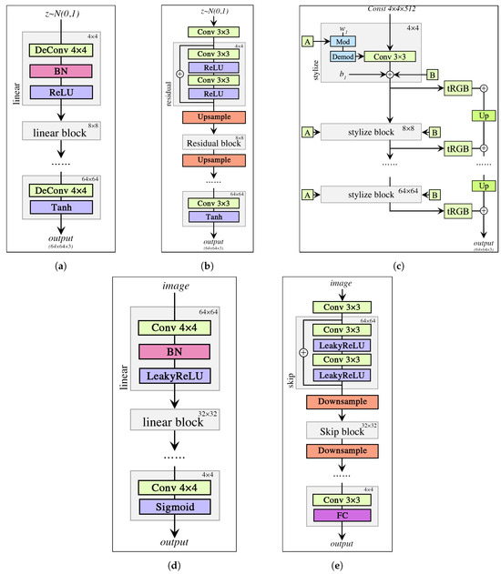
Figure 10.
Taking 64 × 64 resolution RGB image generation as an example, we provide a portrayal of the network structures employed by the SoftGAN in Section 6.5. The generator configurations encompass a linear convolutional design, a residual block-infused architecture and a style block-oriented structure. Meanwhile, the discriminator setups encompass a linear convolutional framework and a skip architecture enriched with residual blocks. Notably, both of these architectures seamlessly integrate with our dynamic borderline softening mechanism, requiring no modifications. (a) Linear generator. (b) ResNet generator. (c) Style generator (synthetic subnetwork part). (d) Linear discriminator. (e) Skip discriminator.
Table 6.
FIDs (where lower values indicate better performance) are reported for three datasets across various network architectures. The best performance achieved within each network architecture is highlighted in bold.
Now, we proceed to examine the experimental outcomes utilizing identical network architectures and adversarial loss. Following 100 epochs of training, we present the FID scores achieved by our SoftGAN model across the CIFAR-10 [30], STL-10 [45] and CelebA [46] datasets. We exclusively incorporate models trained in a fully unsupervised manner to ensure a fair comparison. In summary, our proposed model surpasses the baseline models and achieves a state-of-the-art performance within the same architectural configurations.
Linear generator + linear discriminator: Our architecture closely adheres to the principles of DCGAN [2] for an optimal performance. To ensure effective adversarial learning, we employ hinge loss, which aligns with the SNGAN framework [23]. Impressively, our approach achieves a remarkable FID score of 21.34 on the CIFAR-10 [30] dataset, surpassing other GAN models utilizing the same linear architecture. This includes single-discriminator models, like DCGAN [2], WGAN-GP [14], QSNGAN [49] and SNGAN [23], as well as multi-discriminator models, like Dropout-GAN [24] and MGAN [37]. However, the advantage of our approach on the STL-10 [45] dataset is not as pronounced. It appears that the learning capacity of simple linear networks may be limited when dealing with complex datasets. Despite this, the performance differences among all models are relatively small. Conversely, when evaluating the CelebA [46] dataset, the superiority of the SoftGAN becomes evident once again. Our SoftGAN, implemented within the linear network architecture, achieves a comparable or even superior performance compared to other GAN models employing more intricate networks, such as ResNet and style architectures.
ResNet generator + skip discriminator: When leveraging a more powerful learning-capable network such as ResNet [19], our approach outperforms BigGAN [42] with a notable margin, achieving an FID score of 12.50 on the CIFAR-10 dataset [30]. It stands as the second-best model, surpassed only by AutoGAN [50] with an FID score of 12.42. Regarding the adversarial loss employed in the SoftGAN, we adopt a loss function consistent with WGAN-GP [14]. However, it is worth noting that the inclusion of self-attention layers and the 8-fold increase in batch size in BigGAN impose substantial hardware and training time requirements, surpassing those of our SoftGAN. Similarly, the optimal network architecture search process in AutoGAN also extends its training time beyond that of the SoftGAN. Consequently, the SoftGAN exhibits clear advantages in terms of hardware requirements and training resource consumption while achieving a comparable generation quality. In comparison to PeerGAN [36], a multi-discriminator model, its generation capability falls significantly behind. The experimental results on STL-10 [45] and CelebA [46] datasets echo those of CIFAR-10 [30], demonstrating the robust and competitive performance of the SoftGAN across different datasets.
Style generator + linear discriminator: As the basis for our comparative analysis, we adopt StyleGAN2 [20,21], widely recognized as the most powerful convolutional generative GAN model currently available. With the exception of the dynamic borderline softening mechanism unique to our SoftGAN, the training parameters of StyleGAN2 and our model remain identical. These parameters include the batch size (32) and the optimizer (Adam [29]), as well as the incorporation of style loss, path length regularization and lazy R1 regularization. Notably, our SoftGAN outperforms the current state-of-the-art convolutional style-based GAN models across all three datasets. This achievement effectively demonstrates the superiority of the dynamic borderline softening mechanism when combined with the style network architecture.
7. Conclusions
We present the SoftGAN, an innovative method that tackles the challenges of training instability and mode collapse in GANs by incorporating a dynamic borderline softening mechanism. The core principles of this mechanism are based on optimizing the coverage and expected entropy within fuzzy concept learning. In the SoftGAN, the discriminator aims to learn a fuzzy concept of real data with a smooth transition between real and generated data. During the initial training phase of the SoftGAN, the focus is on maximizing the expected entropy of fuzzy concepts to guide the learning process due to the significant disparity between the generated and real data. However, in the later stages of training, the emphasis shifts to maximizing the concept coverage as the difference between the two distributions diminishes. Our study highlights the effectiveness of the SoftGAN in enhancing both the quality of generated outputs and the robustness across various network architectures. Additionally, we provide empirical evidence showcasing the efficacy of our approach in mitigating the mode collapse problem. Anticipating that our findings may pave the way for an improved modeling performance on extensive image datasets, we also advocate for the application of the dynamic borderline softening mechanism in conjunction with other training techniques.
Author Contributions
Conceptualization, Y.T. and W.L.; investigation, W.L.; software, W.L.; writing—original draft preparation, W.L.; writing—review and editing, Y.T. and W.L.; supervision, Y.T. All authors have read and agreed to the published version of this manuscript.
Funding
This work was funded by the National Natural Science Foundation of China (NO. 61773336, NO. 61961038, NO. 52175253), the National Social Science Foundation of China - Art Project - Major Project (Grant No. 22ZD17), the Modern Design and Cultural Research Center Key Project of Sichuan Province Social Science Key Research Base (Grant No. MD23Z004), Natural Science Foundation of Sichuan Province of China (NO. 22NSFSC0865) and the Art and Engineering Integration Project of Southwest Jiaotong University (Grant No. YG2022010).
Institutional Review Board Statement
Not applicable.
Informed Consent Statement
Not applicable.
Data Availability Statement
The data presented in this study are openly available in CIFAR-10 at https://www.cs.toronto.edu/~kriz/cifar.html [30], LSUN bedroom dataset at https://github.com/fyu/lsun?tab=readme-ov-file [31], STL-10 at https://cs.stanford.edu/~acoates/stl10/ [45], CelebA at https://mmlab.ie.cuhk.edu.hk/projects/CelebA.html [46] and ImageNet at https://www.image-net.org/challenges/LSVRC/2012/ [41].
Acknowledgments
We would like to extend our gratitude to the data providers.
Conflicts of Interest
The authors declare no conflicts of interest.
References
- Goodfellow, I.J.; Pouget-Abadie, J.; Mirza, M.; Xu, B.; Warde-Farley, D.; Ozair, S.; Courville, A.C.; Bengio, Y. Generative Adversarial Nets. In Proceedings of the Advances in Neural Information Processing Systems (NIPS), Montreal, QC, Canada, 8–13 December 2014. [Google Scholar]
- Radford, A.; Metz, L.; Chintala, S. Unsupervised representation learning with deep convolutional generative adversarial networks. In Proceedings of the International Conference on Learning Representations (ICLR), San Juan, PR, USA, 2–4 May 2016. [Google Scholar]
- Arjovsky, M.; Chintala, S.; Bottou, L. Wasserstein generative adversarial networks. In Proceedings of the 34th International Conference on Machine Learning (ICML), Sydney, Australia, 6–11 August 2017; pp. 214–223. [Google Scholar]
- Dong, H.W.; Hsiao, W.Y.; Yang, L.C.; Yang, Y.H. MuseGAN: Multi-track sequential generative adversarial networks for symbolic music generation and accompaniment. In Proceedings of the AAAI Conference on Artificial Intelligence (AAAI), New Orleans, LA, USA, 2–7 February 2018. [Google Scholar]
- Karras, T.; Aila, T.; Laine, S.; Lehtinen, J. Progressive growing of gans for improved quality, stability, and variation. In Proceedings of the International Conference on Learning Representations (ICLR), Vancouver, BC, Canada, 30 April–3 May 2018. [Google Scholar]
- Pumarola, A.; Agudo, A.; Martinez, A.; Sanfeliu, A.; Moreno-Noguer, F. GANimation: Anatomically-aware Facial Animation from a Single Image. In Proceedings of the European Conference on Computer Vision (ECCV), Munich, Germany, 8–14 September 2018. [Google Scholar]
- Zhu, J.Y.; Park, T.; Isola, P.; Efros, A.A. Unpaired Image-To-Image Translation Using Cycle-Consistent Adversarial Networks. In Proceedings of the IEEE International Conference on Computer Vision (ICCV), Venice, Italy, 22–29 October 2017. [Google Scholar]
- Ledig, C.; Theis, L.; Huszar, F.; Caballero, J.; Cunningham, A.; Acosta, A.; Aitken, A.; Tejani, A.; Totz, J.; Wang, Z.; et al. Photo-Realistic Single Image Super-Resolution Using a Generative Adversarial Network. In Proceedings of the IEEE Conference on Computer Vision and Pattern Recognition (CVPR), Honolulu, HI, USA, 21–26 July 2017. [Google Scholar]
- Zhong, Z.; Li, J. Generative Adversarial Networks and Probabilistic Graph Models for Hyperspectral Image Classification. In Proceedings of the AAAI Conference on Artificial Intelligence (AAAI), New Orleans, LA, USA, 2–7 February 2018. [Google Scholar]
- Zadeh, L.A. Fuzzy sets. Inf. Control 1965, 8, 3. [Google Scholar] [CrossRef]
- Lawry, J.; Tang, Y. Uncertainty modelling for vague concepts: A prototype theory approach. Artif. Intell. 2009, 173, 1539–1558. [Google Scholar] [CrossRef]
- Tang, Y.; Xiao, Y. Learning fuzzy semantic cell by principles of maximum coverage, maximum specificity, and maximum fuzzy entropy of vague concept. Knowl.-Based Syst. 2017, 133, 122–140. [Google Scholar] [CrossRef]
- Khrulkov, V.; Oseledets, I. Geometry Score: A Method For Comparing Generative Adversarial Networks. In Proceedings of the 35th International Conference on Machine Learning (ICML), Stockholm, Sweden, 10–15 July 2018. [Google Scholar]
- Gulrajani, I.; Ahmed, F.; Arjovsky, M.; Dumoulin, V.; Courville, A.C. Improved Training of Wasserstein GANs. In Proceedings of the Advances in Neural Information Processing Systems (NIPS), Long Beach, CA, USA, 4–9 December 2017. [Google Scholar]
- Sharma, R.; Barratt, S.; Ermon, S.; Pande, V. Improved Training with Curriculum GANs. arXiv 2018, arXiv:1807.09295. [Google Scholar]
- Petzka, H.; Fischer, A.; Lukovnicov, D. On the regularization of Wasserstein GANs. In Proceedings of the International Conference on Learning Representations (ICLR), Vancouver, BC, Canada, 30 April–3 May 2018. [Google Scholar]
- Creswell, A.; White, T.; Dumoulin, V.; Arulkumaran, K.; Sengupta, B.; Bharath, A.A. Generative adversarial networks: An overview. IEEE Signal Process. Mag. 2018, 35, 53–65. [Google Scholar] [CrossRef]
- Wei, X.; Gong, B.; Liu, Z.; Lu, W.; Wang, L. Improving the Improved Training of Wasserstein GANs: A Consistency Term and Its Dual Effect. In Proceedings of the International Conference on Learning Representations (ICLR), Vancouver, BC, Canada, 30 April–3 May 2018. [Google Scholar]
- He, K.; Zhang, X.; Ren, S.; Sun, J. Deep residual learning for image recognition. In Proceedings of the IEEE Conference on Computer Vision and Pattern Recognition (CVPR), Las Vegas, NV, USA, 27–30 June 2016; pp. 770–778. [Google Scholar]
- Karras, T.; Laine, S.; Aila, T. A style-based generator architecture for generative adversarial networks. In Proceedings of the IEEE/CVF Conference on Computer Vision and Pattern Recognition (CVPR), Long Beach, CA, USA, 15–20 June 2019; pp. 4401–4410. [Google Scholar]
- Karras, T.; Laine, S.; Aittala, M.; Hellsten, J.; Lehtinen, J.; Aila, T. Analyzing and improving the image quality of Stylegan. In Proceedings of the IEEE/CVF Conference on Computer Vision and Pattern Recognition (CVPR), Seattle, WA, USA, 13–19 June 2020; pp. 8110–8119. [Google Scholar]
- Karras, T.; Aittala, M.; Hellsten, J.; Laine, S.; Lehtinen, J.; Aila, T. Training generative adversarial networks with limited data. In Proceedings of the Advances in Neural Information Processing Systems (NIPS), Virtual, 6–12 December 2020; Volume 33, pp. 12104–12114. [Google Scholar]
- Miyato, T.; Kataoka, T.; Koyama, M.; Yoshida, Y. Spectral Normalization for Generative Adversarial Networks. In Proceedings of the International Conference on Learning Representations (ICLR), Vancouver, BC, Canada, 30 April–3 May 2018. [Google Scholar]
- Mordido, G.; Yang, H.; Meinel, C. Dropout-GAN: Learning from a Dynamic Ensemble of Discriminators. In Proceedings of the International Conference on Knowledge Discovery and Data Mining, London, UK, 19–23 August 2018. [Google Scholar]
- Nguyen, T.; Le, T.; Vu, H.; Phung, D. Dual Discriminator Generative Adversarial Nets. In Proceedings of the Advances in Neural Information Processing Systems (NIPS), Long Beach, CA, USA, 4–9 December 2017; pp. 2670–2680. [Google Scholar]
- Durugkar, I.; Gemp, I.; Mahadevan, S. Generative Multi-Adversarial Networks. In Proceedings of the International Conference on Learning Representations (ICLR), Toulon, France, 24–26 April 2017. [Google Scholar]
- Wei, J.; Liu, M.; Luo, J.; Li, Q.; Davis, J.; Liu, Y. DuelGAN: A Duel Between Two Discriminators Stabilizes the GAN Training. In Proceedings of the European Conference on Computer Vision (ECCV), Tel Aviv, Israel, 23–27 October 2022. [Google Scholar]
- Rubner, Y.; Tomasi, C. The Earth Mover’s Distance. In Perceptual Metrics for Image Database Navigation; Springer: Berlin/Heidelberg, Germany, 2001; pp. 13–28. [Google Scholar]
- Kingma, D.; Ba, J. Adam: A method for stochastic optimization. In Proceedings of the International Conference on Learning Representations (ICLR), Banff, AB, Canada, 14–16 April 2014. [Google Scholar]
- Krizhevsky, A.; Hinton, G. Learning Multiple Layers of Features from Tiny Images; Technical Report; Citeseer: Toronto, ON, Canada, 2009. [Google Scholar]
- Yu, F.; Zhang, Y.; Song, S.; Seff, A.; Xiao, J. LSUN: Construction of a Large-scale Image Dataset using Deep Learning with Humans in the Loop. arXiv 2015, arXiv:1506.03365. [Google Scholar]
- Warde-Farley, D.; Bengio, Y. Improving generative adversarial networks with denoising feature matching. In Proceedings of the International Conference on Learning Representations (ICLR), Toulon, France, 24–26 April 2017. [Google Scholar]
- Dumoulin, V.; Belghazi, I.; Poole, B.; Mastropietro, O.; Lamb, A.; Arjovsky, M.; Courville, A. Adversarially learned inference. In Proceedings of the International Conference on Learning Representations (ICLR), Toulon, France, 24–26 April 2017. [Google Scholar]
- Berthelot, D.; Schumm, T.; Metz, L. Began: Boundary equilibrium generative adversarial networks. arXiv 2017, arXiv:1703.10717. [Google Scholar]
- Salimans, T.; Goodfellow, I.; Zaremba, W.; Cheung, V.; Radford, A.; Chen, X. Improved techniques for training gans. In Proceedings of the Advances in Neural Information Processing Systems (NIPS), Barcelona, Spain, 5–10 December 2016; pp. 2234–2242. [Google Scholar]
- Wei, J.; Liu, M.; Luo, J.; Li, Q.; Davis, J.; Liu, Y. PeerGAN: Generative Adversarial Networks with a Competing Peer Discriminator. arXiv 2021, arXiv:2101.07524. [Google Scholar]
- Quan, H.; Tu, D.N.; Trung, L.; Ding, P. MGAN:Traning Generative Adversarial Nets with Multiple Generators. In Proceedings of the International Conference on Learning Representations (ICLR), Vancouver, BC, Canada, 30 April–3 May 2018. [Google Scholar]
- Zhang, H.; Zhang, Z.; Odena, A.; Lee, H. Consistency regularization for generative adversarial networks. In Proceedings of the International Conference on Learning Representations (ICLR), Addis Ababa, Ethiopia, 26–30 April 2020. [Google Scholar]
- Song, Y.; Ye, Q.; Xu, M.; Liu, T.-Y. Discriminator Contrastive Divergence: Semi-Amortized Generative Modeling by Exploring Energy of the Discriminator. In Proceedings of the International Conference on Learning Representations Deep Inverse Workshop (ICLR-W), Virtual, 6–12 December 2020. [Google Scholar]
- Bao, H.; Dong, L.; Wei, F. BEiT: BERT Pre-Training of Image Transformers. arXiv 2021, arXiv:2106.08254. [Google Scholar]
- Russakovsky, O.; Deng, J.; Su, H.; Krause, J.; Satheesh, S.; Ma, S.; Huang, Z.; Karpathy, A.; Khosla, A.; Bernstein, M.; et al. ImageNet Large Scale Visual Recognition Challenge. Int. J. Comput. Vis. (IJCV) 2015, 115, 211–252. [Google Scholar] [CrossRef]
- Brock, A.; Donahue, J.; Simonyan, K. Large Scale GAN Training for High Fidelity Natural Image Synthesis. In Proceedings of the International Conference on Learning Representations (ICLR), New Orleans, LA, USA, 6–9 May 2019. [Google Scholar]
- Paszke, A.; Gross, S.; Chintala, S.; Chanan, G.; Yang, E.; DeVito, Z.; Lin, Z.; Desmaison, A.; Antiga, L.; Lerer, A. Automatic differentiation in PyTorch. In Proceedings of the Advances in Neural Information Processing Systems Workshop (NeurIPS-W), Long Beach, CA, USA, 4–9 December 2017. [Google Scholar]
- Huang, X.; Li, Y.; Poursaeed, O.; Hopcroft, J.; Belongie, S. Stacked generative adversarial networks. In Proceedings of the IEEE Conference on Computer Vision and Pattern Recognition (CVPR), Honolulu, HI, USA, 21–26 July 2017; pp. 5077–5086. [Google Scholar]
- Coates, A.; Ng, A.; Lee, H. An analysis of single-layer networks in unsupervised feature learning. In Proceedings of the Fourteenth International Conference on Artificial Intelligence and Statistics, Ft. Lauderdale, FL, USA, 11–13 April 2011; pp. 215–223. [Google Scholar]
- Liu, Z.; Luo, P.; Wang, X.; Tang, X. Deep Learning Face Attributes in the Wild. In Proceedings of the IEEE International Conference on Computer Vision (ICCV), Santiago, Chile, 7–13 December 2015; pp. 3730–3738. [Google Scholar]
- Heusel, M.; Ramsauer, H.; Unterthiner, T.; Nessler, B.; Hochreiter, S. GANs Trained by a Two Time-Scale Update Rule Converge to a Local Nash Equilibrium. In Proceedings of the Advances in Neural Information Processing Systems (NeurIPS), Long Beach, CA, USA, 4–9 December 2017; pp. 6626–6637. [Google Scholar]
- Szegedy, C.; Liu, W.; Jia, Y.; Sermanet, P.; Reed, S.; Anguelov, D.; Erhan, D.; Vanhoucke, V.; Rabinovich, A. Going deeper with convolutions. In Proceedings of the IEEE Conference on Computer Vision and Pattern Recognition (CVPR), Boston, MA, USA, 7–12 June 2015; pp. 1–9. [Google Scholar]
- Grassucci, E.; Cicero, E.; Comminiello, D. Quaternion generative adversarial networks. In Generative Adversarial Learning: Architectures and Applications; Springer: Berlin/Heidelberg, Germany, 2022; pp. 57–86. [Google Scholar]
- Gong, X.; Chang, S.; Jiang, Y.; Wang, Z. Autogan: Neural architecture search for generative adversarial networks. In Proceedings of the IEEE/CVF International Conference on Computer Vision (ICCV), Seoul, Republic of Korea, 27 October–2 November 2019; pp. 3224–3234. [Google Scholar]
- Patel, P.; Kumari, N.; Singh, M.; Krishnamurthy, B. LT-GAN: Self-Supervised GAN with Latent Transformation Detection. In Proceedings of the IEEE/CVF Winter Conference on Applications of Computer Vision (WACV), Waikoloa, HI, USA, 3–8 January 2021; pp. 3189–3198. [Google Scholar]
Disclaimer/Publisher’s Note: The statements, opinions and data contained in all publications are solely those of the individual author(s) and contributor(s) and not of MDPI and/or the editor(s). MDPI and/or the editor(s) disclaim responsibility for any injury to people or property resulting from any ideas, methods, instructions or products referred to in the content. |
© 2024 by the authors. Licensee MDPI, Basel, Switzerland. This article is an open access article distributed under the terms and conditions of the Creative Commons Attribution (CC BY) license (https://creativecommons.org/licenses/by/4.0/).