State Estimation for Measurement-Saturated Memristive Neural Networks with Missing Measurements and Mixed Time Delays Subject to Cyber-Attacks: A Non-Fragile Set-Membership Filtering Framework

Abstract

This paper is concerned with the state estimation problem based on non-fragile set-membership filtering for a class of measurement-saturated memristive neural networks (MNNs) with unknown but bounded (UBB) noises, mixed time delays and missing measurements (MMs), subject to cyber-attacks under the framework of weighted try-once-discard protocol (WTOD protocol). Considering bandwidth-limited open networks, this paper proposes an improved set-membership filtering based on WTOD protocol to partially solve the problem that multiple sensor-related problems and multiple network-induced phenomena influence the state estimation performance of MNNs. Moreover, this paper also discusses the gain perturbations of the estimator and proposes an improved non-fragile estimation framework based on set-membership filtering, which enhances the robustness of the estimation approach. The proposed estimation framework can effectively estimate the state of MNNs with UBB noises, estimator gain perturbations, mixed time-delays, cyber-attacks, measurement saturations and MMs. This paper first utilizes mathematical induction to provide the sufficient conditions for the existence of the desired estimator, and obtains the estimator gain by solving a set of linear matrix inequalities. Then, a recursive optimization algorithm is utilized to achieve optimal estimation performance. The effectiveness of the theoretical results is verified by comparative numerical simulation examples.

1. Introduction

In circuit theory, the memristor is the fourth novel passive nano-information device, after the three basic circuit components of inductor, capacitor and resistor, which has the functions of memory and resistance. Studies have found that the memory characteristics of memristor can reflect well the excitation and inhibition of synapses in artificial neural networks (ANNs) [1]. Therefore, memristive neural networks (MNNs), which utilize the memristor to replace the synapse in the ANNs, have attracted the extensive attention of scholars. MNNs are extensively employed in intelligent control, signal processing, pattern recognition, etc. Nonetheless, with increasing network size and complexity, various faults and disturbances may occur in MNNs. If these faults and disturbances are not promptly estimated to make the system adjust as early as possible, the performance of the MNNs will decay or even collapse. Therefore, the state estimation of MNNs has gained some attention from academic research communities. For example, corresponding estimation approaches have been designed to estimate various MNNs, such as random delayed MNNs [2], Markov switching MNNs [3] and proportional delayed complex-valued MNNs [4].

Dealing with the state estimation problem has two main kinds of approaches, namely, filter and observer. Among them, the filter has been widely used in the state estimation domain related to MNNs owing to its superior noise resistance [5,6]. Different filtering strategies need to be selected for the different types of noise. Currently, most of the literature on filtering only considers white Gaussian noise and energy-bounded noise in MNNs. White Gaussian noise obeys the Gaussian distribution, and the primary processing techniques include recursive filtering [7], particle filtering [8], etc. Energy-bounded noise has bounded energy, and the primary processing techniques include $H_{\infty }$ filtering [9], energy-to-peak filtering [10], etc. However, system operation may generate unknown but bounded (UBB) noise in reality, such as electromagnetic systems that can produce the UBB noise in electrical engineering, which does not follow either the assumption of a Gaussian distribution or bounded energy. For UBB noise, the traditional state estimation approaches become no longer applicable. Therefore, the set-membership filtering (SMF) was proposed to deal with these kinds of noises [11]. Compared to other filters, the SMF only requires a strict boundary constraint on noise rather than statistical characteristics and can give a group of ellipsoid sets that encompass all possible actual states with a 100% confidence degree. There have been many research results on using SMF to deal with UBB noise. For example, in response to the following various systems with UBB noise, such as multi-sensor network system [12], distributed nonlinear discrete system [13], time-varying system [14], nonlinear system [15] and event-triggered complex networks [16], the corresponding set-membership estimation schemes have been designed to estimate the state of the above systems. In an actual engineering scenario, ref. [17] has proposed a control scheme based on SMF to tackle the heading tracking control problem in an unmanned surface vessel (USV) affected by UBB noise, which guarantees the asymptotic stability of the USV systems. In [18], an SMF has been proposed to track the running trajectory of automatic guided vehicle (AGV) under UBB noise, which decreases the requirement for sensor precision. From the above, we can see that there have been some good research results on SMF. What is noteworthy is that the existing research has not considered some special practical problems fully, such as the uncertainty problems in engineering scenarios.

In fact, in real engineering application scenarios, estimation performance is unavoidably influenced by uncertainties such as actuator degradation, numerical calculation errors and the aging of components. The presence of these uncertainties can cause gain perturbation in the estimator and can result in a decrease in the overall estimation performance, so such an estimator is also called a “fragile” estimator. To ensure the robustness of the estimator, the non-fragility need to be fully considered during the design process. In the past few years, there has been much attention from scholars on the non-fragile set-membership estimation of MNNs. In [19], a non-fragile estimation approach based on SMF for MNNs with logarithmic quantization has been proposed under the framework of Maximum Error First protocol. A non-fragile estimation approach has been proposed for discrete measurement-saturated MNNs based on set-membership filtering under the framework of weighted try-once-discard (WTOD) protocol [20]. In [21], a non-fragile distributed secure SMF framework has been designed to estimate nonlinear systems influenced by channel fading and cyber-attacks. However, it is worth noting that, under the framework of non-fragile estimation based on SMF, the main structure of the linear matrix inequality (LMI) for estimating the error changes significantly when the system is suffering from stochastic cyber-attacks. Therefore, the matrix blocks of the non-fragile parts that deal with the parameter uncertainty and the estimator gain perturbation also need to be changed along with the change of main structure. Based on our knowledge, we have not seen research reports concerning the non-fragile estimation based on SMF for MNNs under stochastic cyber-attacks. Moreover, alongside the aforementioned gain perturbation, the use of the communication network and inferior sensors also brings some detrimental influences on the state estimation problem of MNNs despite its numerous conveniences.

The inferior sensors mentioned above are cheap, but, due to their physical limitations and the influence of intermittent faults, encountering sensor-related problems is inevitable during the measuring process of the system, such as measurement saturations and missing measurements (MMs). The occurrence of these sensor-related problems can influence the estimation performance seriously. Therefore, scholars have conducted research on the problem of set-membership estimation when measurement saturations and MMs exist from different perspectives. For time-varying systems influenced by sensor saturation, refs. [22,23] have proposed corresponding event-based distributed set-membership filters and controllers, respectively. Reference [24] has reviewed various processing approaches for systems influenced by measurement saturation and MMs. For a class of discrete nonlinear systems influenced by measurement saturation and MMs simultaneously, ref. [25] has proposed a distributed filter based on a random access (RA) protocol. A sector-bounded approach has been employed to partition the saturation function into linear and nonlinear components to deal with the saturation phenomena for the sensor-saturated systems; then, an SMF was designed for state estimation in [26]. In [27], a recursive joint state and fault estimation (JSFE) filter based on the Round-Robin (RR) protocol has been designed for a class of nonlinear systems with MMs and random component faults. Reference [28] has studied an $H_{\infty }$ filter problem for a class of uncertain stochastic nonlinear systems with probabilistic MMs, time-delays and external random disturbances. However, currently, most of the literature only considers these sensor-related problems; there exists little research on reducing the influence of these problems on the estimation of performance. How to solve this problem to a certain extent is a research motivation of this paper.

The network communication mentioned above has the advantages of easy maintenance and low modularity, which reduce communication costs during data transmission effectively. However, due to the limited communication capacity of the network and the lack of channel protection measures, various network-induced phenomena are inevitably encountered in the process of data transmission, such as time delays, cyber-attacks and packet loss. Network-induced phenomena can raise the instability factor of the system and reduce the performance of the estimator [29]. Therefore, estimating these phenomena timely and reducing their influence on estimation performance as far as possible has important practical meaning. For a variety of network-induced phenomena that occur in engineering practice, such as various measurement and state value anomalies (state saturation [30], constrained measurement [31], measurement outliers [32]) and various cyber-attacks (malicious attacks that can bypass anomaly detectors [33], deception attack [34], joint false data injection attack [35], replay attack [36], DoS attack [37,38] and mixed-attacks [39]), the corresponding estimation schemes have been designed to reduce the influence of the above phenomena on the estimation performance. Scholars have conducted research on the problem of set-membership estimation with network-induced phenomena from different perspectives. For example, to overcome the communication constraints, refs. [40,41] have designed the corresponding SMF in the case of introducing redundant channels. In view of the incomplete data caused by various factors in the transmission process, refs. [42,43] have used censored measurement to describe this phenomenon and have designed the corresponding SMF. For the actual engineering scenarios, a state estimation approach that utilizes the Kalman filter and recursive systematic convolutional code has been proposed in [44] to effectively estimate the state of the smart grid and detect attacks, which guarantees the normal operation of the smart grid. In [45], a particle filter based on the Paillier encryption–decryption scheme has been proposed for the multi-machine power systems for confronting the potential risk of cyber-attacks, which makes the attacker unable to attack the encrypted data to ensure the precision of state estimation during the operation of the multi-machine power systems.

In fact, several studies have considered the various sensor-related problems and network-induced phenomena mentioned above, and have given hypotheses for corresponding approaches. For MMs, ref. [46] has given the hypothesis that MMs must satisfy the binary exchange sequence of the conditional probability distribution. Reference [27] has given the hypothesis that MMs need to satisfy Bernoulli distribution. Reference [28] has given the hypothesis that the occurrence of different MMs in each sensor node can be described by a diagonal matrix, which is more realistic. Regarding cyber-attacks, many scholars have hypothesized that cyber-attacks obey the hidden Markov model [47]. However, since the Bernoulli distribution can directly indicate whether the attack occurs through the value of the random variable (0 or 1) [48], which is more suitable to describe the deception attack. Therefore, this paper also hypothesizes that the cyber-attacks follow the Bernoulli distribution and uses a diagonal matrix to describe the continuous occurrence of the MMs on different sensor nodes.

From the aforementioned and related literature, we can see that current studies only consider the set-membership estimation of MNNs encountering either various sensor related problems or various network-induced phenomena. As far as we know, we have not yet seen the research results on how to conduct set-membership estimation and reduce the influence on state estimation performance when the MNNs encounter multiple sensor-related problems and multiple network-induced phenomena simultaneously.

To solve the aforementioned difficulties, considering that the communication protocol only allows one sensor node to send the latest data to the estimator during each sampling instant, we propose utilizing network protocol to partially solve the problem that the state estimation performance influenced by the MMs and bandwidth limitation for MNNs. The common communication protocols mainly include RA protocol [49,50,51], RR protocol [52,53] and WTOD protocol [54,55,56,57,58,59,60]. Among them, the WTOD protocol is regarded as the most efficacious protocol [55], which can give the priority to sending the latest data to sensor nodes according to the principle of “most needed” to find the sensor node that has the maximum difference between the measured output at the present sampling instant and that of the preceding sampling instant. Therefore, this paper proposes an improved SMF algorithm based on the WTOD protocol to partially solve the influencing problem of multiple sensor-related problems and multiple network-induced phenomena on estimation performance. The difficulty in doing so is because the introduction of the WTOD protocol increases the complexity and nonlinearity of the system model, which brings significant challenge for the design and performance analysis of the estimator.

In view of the preceding problem and practical requirements, this paper estimates the states of MNNs with mixed time delays, measurement saturations, MMs and gain perturbations of the estimator subject to cyber-attacks under the framework of the WTOD protocol. A non-fragile set-membership estimator is designed. The primary contributions of this paper are threefold: (1) Compared with [20], more sensor-related problems and network-induced phenomena are considered in MNNs, including cyber-attacks and MMs, which makes the established model more realistic; (2) Compared with [27], we propose that using an improved set-membership estimation algorithm based on the WTOD protocol to partially solve the difficulty of set-membership estimation in the presence of network-induced phenomena and sensor-related problems in MNNs, which can reduce both the influence of network congestion under bandwidth limitation and the MMs on state estimation; (3) Considering the introduction of stochastic variables, we improve the traditional non-fragile estimation frameworks in [19,20] to handle the simultaneous occurrence of gain perturbation and parameter uncertainty in MNNs.

The subsequent structure of this paper is organized as follows. Section 2 introduces the MNN model and designs the corresponding non-fragile estimator. The sufficient condition and proof process are provided in Section 3 for the existence of the non-fragile estimator. The parameters of the non-fragile estimator are derived through the solution of a set of LMIs. Section 4 provides the evidence to support the effectiveness and feasibility of the proposed estimation algorithm through the use of numerical examples. Section 5 gives a comprehensive overview of this paper.

Notation. ∗ represents the transposed term of symmetry in the symmetric block matrix. ${\mathrm{R}}^{n_x}$ represents $n_x$-dimensional Euclidean space. $U^{-1}$ and $\Vert U\Vert$ represent the inverse and 2-norm of the matrix U, respectively. I indicates the identity matrix with proper dimensions. $\varphi \ge Z$$(\varphi >Z)$ means that $\varphi -Z$ is positive semi-definite (positive definite). $\mathrm{E}\{·\}$ represents the mathematical expectation. The $\mathrm{trace}\left(N\right)$ is the trace of the matrix N. $\mathrm{P}\left\{B\right\}$ is the occurrence probability of the event ‘B’. $\mathrm{diag}\{·\}$ indicates a block diagonal matrix. The superscript “T” denotes the transpose operation. $A\in [{\wp }^{-},{\wp }^{+}]$ indicates that the value of every element in A falls within the specified interval $[{\wp }^{-},{\wp }^{+}]$, i.e., between the upper bound denoted as ${\wp }^{+}$ and the lower bound denoted as ${\wp }^{-}$. The highest value and the lowest value are represented as $\max \{·,·\}$ and $\min \{·,·\}$, respectively.

2. Problem Formulation

In this section, we first consider a class of discrete measurement-saturated MNNs with mixed time delays in the following [20]:

$$\left\{\begin{array}{c}{\overline{\tilde{o}}}_{u+1}=\overline{\tilde{A}}\left({\overline{\tilde{o}}}_u\right){\overline{\tilde{o}}}_u+\overline{\tilde{B}}\left({\overline{\tilde{o}}}_u\right)f\left({\overline{\tilde{o}}}_u\right)+\overline{\tilde{D}}\left({\overline{\tilde{o}}}_u\right)g\left({\overline{\tilde{o}}}_{u-{\tau }_1}\right)\hfill \\ +\overline{\tilde{E}}\left({\overline{\tilde{o}}}_u\right)\underset{i=1}{\sum ^{{\tau }_2}}{\mu }_i{\overline{\tilde{o}}}_{u-i}+{\overline{\tilde{H}}}_w{\overline{\tilde{W}}}_u,\hfill \\ {\tilde{q}}_u=\Gamma \left(\overline{\tilde{C}}{\overline{\tilde{o}}}_u\right)+{\overline{\tilde{H}}}_v{\overline{\tilde{V}}}_u,\hfill \\ {\overline{\tilde{o}}}_u={\overline{\Psi }}_u,u\in [-\tau ,0],\tau =max\{{\tau }_1,{\tau }_2\},\hfill \end{array}\right.$$

(1)

where ${\overline{\tilde{o}}}_u={[{\overline{\tilde{o}}}_{1,u},{\overline{\tilde{o}}}_{2,u},\cdots ,{\overline{\tilde{o}}}_{n_x,u}]}^{\mathrm{T}}\in {\mathrm{R}}^{n_x}$ is the state vector of $n_x$ neurons with initial value ${\overline{\Psi }}_u$. ${\tilde{q}}_u={[{\tilde{q}}_{1,u},{\tilde{q}}_{2,u},\cdots ,{\tilde{q}}_{n_y,u}]}^{\mathrm{T}}\in {\mathrm{R}}^{n_y}$ is the measurement output of the MNNs. ${\overline{\tilde{V}}}_u\in {\mathrm{R}}^{n_v}$ and ${\overline{\tilde{W}}}_u\in {\mathrm{R}}^{n_w}$ represent the measurement noise and the process noise, respectively. $f(·)$, $g(·)$ and $\Gamma (·)$ denote the nonlinear functions. $\begin{array}{c}\overline{\tilde{A}}\left({\overline{\tilde{o}}}_u\right)={\mathrm{diag}}_{n_x}\left\{a_i\left({\overline{\tilde{o}}}_{i,u}\right)\right\}\hfill \end{array}$ is the self-feedback matrix with suitable dimension. $\overline{\tilde{B}}\left({\overline{\tilde{o}}}_u\right)={\left(b_{ij}\left({\overline{\tilde{o}}}_{i,u}\right)\right)}_{n_x\times n_x}$ is the connection weight matrix with suitable dimension. $\overline{\tilde{D}}\left({\overline{\tilde{o}}}_u\right)={\left(d_{ij}\left({\overline{\tilde{o}}}_{i,u}\right)\right)}_{n_x\times n_x}$ and $\overline{\tilde{E}}\left({\overline{\tilde{o}}}_u\right)={\left(h_{ij}\left({\overline{\tilde{o}}}_{i,u}\right)\right)}_{n_x\times n_x}$ are the delayed connection weight matrices with suitable dimensions. $\overline{\tilde{C}}$, ${\overline{\tilde{H}}}_w$ and ${\overline{\tilde{H}}}_v$ are the known real-valued matrices with proper dimensions. ${\tau }_1$ represents the determined constant delay. ${\tau }_2$ and ${\mu }_i$$(i=1,2,\cdots ,{\tau }_2)$ represent the distributed delay, which is caused by the delay accumulation influences of real circuit components and exists in MNNs widely.

Assumption 1.

The process noise ${\overline{\tilde{W}}}_u\in {\mathrm{R}}^{n_w}$ in the first formula in (1) and the measurement noise ${\overline{\tilde{V}}}_u\in R^{n_v}$ in the second formula of (1) are UBB noises, which are restricted to the ellipsoidal sets specified below:

$$\left\{\begin{array}{c}{z}_{w_u}=\{{\overline{\tilde{W}}}_u\in R^{n_w}:{\overline{\tilde{W}}}_u^T{R}_{w,u}^{-1}{\overline{\tilde{W}}}_u\le 1\},\hfill \\ z_{v_u}=\{{\overline{\tilde{V}}}_u\in R^{n_v}:{\overline{\tilde{V}}}_u^T{R}_{v,u}^{-1}{\overline{\tilde{V}}}_u\le 1\},\hfill \end{array}\right.$$

(2)

where $R_{w,u}>0$ and $R_{v,u}>0$ are known time-varying matrices with proper dimensions.

The saturation function $\Gamma (·):{\mathrm{R}}^{n_y}\to {\mathrm{R}}^{n_y}$ is defined in the following:

$$\Gamma \left(\overline{\tilde{\sigma }}\right)={\left({\Gamma }_1\left({\overline{\tilde{\sigma }}}_1\right),{\Gamma }_2\left({\overline{\tilde{\sigma }}}_2\right),\cdots ,{\Gamma }_{n_y}\left({\overline{\tilde{\sigma }}}_{n_y}\right)\right)}^{\mathrm{T}},$$

(3)

with ${\Gamma }_t\left({\overline{\tilde{\sigma }}}_t\right)=\mathrm{sign}\left({\overline{\tilde{\sigma }}}_t\right)\min \left\{{\overline{\tilde{\sigma }}}_{t,max},\left|{\overline{\tilde{\sigma }}}_t\right|\right\}$, where ${\overline{\tilde{\sigma }}}_{t,max}$ denotes the t-th element of saturation level ${\overline{\tilde{\sigma }}}_{max}$ and $\mathrm{sign}(·)$ represents the signum function.

Definition 1

([61]). A nonlinear function $\eta (·)$ and real matrices $m_1$ and $m_2$ are given, and $m_2-m_1>0$.

If the particular condition

$${\left(\eta \left(\chi \right)-m_1\chi \right)}^T\left(\eta \left(\chi \right)-m_2\chi \right)\le 0,$$

(4)

holds, then $\eta (·)$ is defined such that it satisfies the sector-bounded condition and belongs to the sector $m_1$ and $m_2$.

According to Definition 2 and Figure 1, the real matrices ${\overline{\tilde{U}}}_1$ and $\overline{\tilde{U}}$ are given and $0\le {\overline{\tilde{U}}}_1<1\le \overline{\tilde{U}}$, which guarantees

$${\left({\Gamma }_t\left({\overline{\tilde{\sigma }}}_{t,u}\right)-{\overline{\tilde{U}}}_1{\overline{\tilde{\sigma }}}_{t,u}\right)}^{\mathrm{T}}\left({\Gamma }_t\left({\overline{\tilde{\sigma }}}_{t,u}\right)-\overline{\tilde{U}}{\overline{\tilde{\sigma }}}_{t,u}\right)\le 0,$$

(5)

where ${\Gamma }_t(·)$ is the sector-bounded nonlinear function, which belongs to $[{\overline{\tilde{U}}}_1,\overline{\tilde{U}}]$.

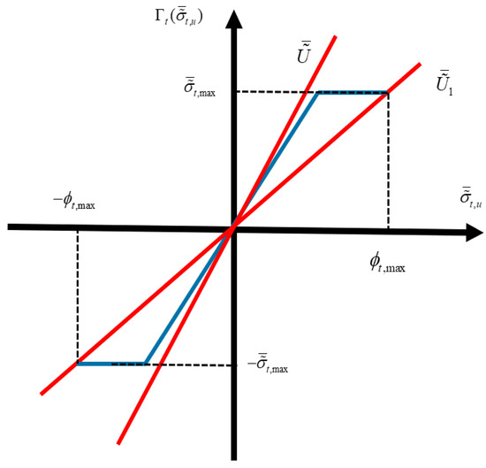
Figure 1. Schematic diagram of sector-bounded nonlinear saturation function.

In practical engineering, there generally exists a vector ${\varphi }_{t,max}\ge {\overline{\tilde{\sigma }}}_{t,u}$. The saturation function ${\Gamma }_t(·)$ can be decomposed into two components: the linear and nonlinear parts, that is,

$${\Gamma }_t\left(\overline{\tilde{C}}{\overline{\tilde{o}}}_u\right)={\overline{\tilde{U}}}_1\overline{\tilde{C}}{\overline{\tilde{o}}}_u+\theta \left(\overline{\tilde{C}}{\overline{\tilde{o}}}_u\right),$$

(6)

where $\theta (\overline{\tilde{C}}{\overline{\tilde{o}}}_u)$ is the sector-bounded nonlinear function belonging to $[0,{\overline{\tilde{U}}}_2]$, in which ${\overline{\tilde{U}}}_2\triangleq \overline{\tilde{U}}-{\overline{\tilde{U}}}_1$. Then, $\theta \left(\overline{\tilde{C}}{\overline{\tilde{o}}}_u\right)$ satisfies:

$${\theta }^{\mathrm{T}}\left(\overline{\tilde{C}}{\overline{\tilde{o}}}_u\right)\left(\theta (\overline{\tilde{C}}{\overline{\tilde{o}}}_u)-{\overline{\tilde{U}}}_2(\overline{\tilde{C}}{\overline{\tilde{o}}}_u)\right)\le 0.$$

(7)

Next, according to [2], we can obtain the state-dependent functions:

$$a_i\left({\overline{\tilde{o}}}_{i,u}\right)=\left\{\begin{array}{c}{\stackrel{⌢}{s}}_i\left|{\overline{\tilde{o}}}_{i,u}\right|>r_i\hfill \\ {\stackrel{⌣}{s}}_i\left|{\overline{\tilde{o}}}_{i,u}\right|\le r_i\hfill \end{array},\right.b_{ij}\left({\overline{\tilde{o}}}_{i,u}\right)=\left\{\begin{array}{c}{\stackrel{⌢}{b}}_{ij}\left|{\overline{\tilde{o}}}_{i,u}\right|>r_i\hfill \\ {\stackrel{⌣}{b}}_{ij}\left|{\overline{\tilde{o}}}_{i,u}\right|\le r_i\hfill \end{array},\right.$$

$$d_{ij}\left({\overline{\tilde{o}}}_{i,u}\right)=\left\{\begin{array}{c}{\stackrel{⌢}{d}}_{ij}\left|{\overline{\tilde{o}}}_{i,u}\right|>r_i\hfill \\ {\stackrel{⌣}{d}}_{ij}\left|{\overline{\tilde{o}}}_{i,u}\right|\le r_i\hfill \end{array},\right.h_{ij}\left({\overline{\tilde{o}}}_{i,u}\right)=\left\{\begin{array}{c}{\stackrel{⌢}{h}}_{ij}\left|{\overline{\tilde{o}}}_{i,u}\right|>r_i\hfill \\ {\stackrel{⌣}{h}}_{ij}\left|{\overline{\tilde{o}}}_{i,u}\right|\le r_i\hfill \end{array},\right.$$

where $r_i>0$, $\left|{\stackrel{⌢}{s}}_i\right|<1$, $|{\stackrel{⌣}{s}}_i|<1$, ${\stackrel{⌢}{b}}_{ij}$, ${\stackrel{⌣}{b}}_{ij}$, ${\stackrel{⌢}{d}}_{ij}$, ${\stackrel{⌣}{d}}_{ij}$, ${\stackrel{⌢}{h}}_{ij}$ and ${\stackrel{⌣}{h}}_{ij}$ are all known scalars.

Denote

$$a_i^{-}=min\{{\stackrel{⌢}{s}}_i,{\stackrel{⌣}{s}}_i\},a_i^{+}=max\{{\stackrel{⌢}{s}}_i,{\stackrel{⌣}{s}}_i\},b_{ij}^{-}=min\{{\stackrel{⌢}{b}}_{ij},{\stackrel{⌣}{b}}_{ij}\},b_{ij}^{+}=max\{{\stackrel{⌢}{b}}_{ij},{\stackrel{⌣}{b}}_{ij}\},$$

$$d_{ij}^{-}=min\{{\stackrel{⌢}{d}}_{ij},{\stackrel{⌣}{d}}_{ij}\},d_{ij}^{+}=max\{{\stackrel{⌢}{d}}_{ij},{\stackrel{⌣}{d}}_{ij}\},h_{ij}^{-}=min\{{\stackrel{⌢}{h}}_{ij},{\stackrel{⌣}{h}}_{ij}\},h_{ij}^{+}=max\{{\stackrel{⌢}{h}}_{ij},{\stackrel{⌣}{h}}_{ij}\},$$

$$A^{-}={\mathrm{diag}}_{n_x}\left\{a_i^{-}\right\},A^{+}={\mathrm{diag}}_{n_x}\left\{a_i^{+}\right\},{\&}^{-}={\left({b^{-}}_{ij}\right)}_{n_x\times n_x},{\&}^{+}={\left({b^{+}}_{ij}\right)}_{n_x\times n_x},$$

$${\upsilon }^{-}={\left({d^{-}}_{ij}\right)}_{n_x\times n_x},{\upsilon }^{+}={\left({d^{+}}_{ij}\right)}_{n_x\times n_x},E^{-}={\left({h^{-}}_{ij}\right)}_{n_x\times n_x},E^{+}={\left({h^{+}}_{ij}\right)}_{n_x\times n_x}.$$

We can obtain that $\overline{\tilde{A}}\left({\overline{\tilde{o}}}_u\right)\in [A^{-},A^{+}]$, $\overline{\tilde{B}}\left({\overline{\tilde{o}}}_u\right)\in [{\&}^{-},{\&}^{+}]$, $\overline{\tilde{D}}\left({\overline{\tilde{o}}}_u\right)\in [{\upsilon }^{-},{\upsilon }^{+}]$ and $\overline{\tilde{E}}\left({\overline{\tilde{o}}}_u\right)\in [E^{-},E^{+}]$. Next, $\overline{\tilde{A}}$, $\overline{\tilde{B}}$, $\overline{\tilde{D}}$ and $\overline{\tilde{E}}$ are defined as follows:

$$\overline{\tilde{A}}\triangleq (A^{+}+A^{-})/2,\overline{\tilde{B}}\triangleq ({\&}^{+}+{\&}^{-})/2,$$

$$\overline{\tilde{D}}\triangleq ({\upsilon }^{+}+{\upsilon }^{-})/2,\overline{\tilde{E}}\triangleq (E^{+}+E^{-})/2.$$

Furthermore, the matrices $\overline{\tilde{A}}\left({\overline{\tilde{o}}}_u\right)$, $\overline{\tilde{B}}\left({\overline{\tilde{o}}}_u\right)$, $\overline{\tilde{D}}\left({\overline{\tilde{o}}}_u\right)$ and $\overline{\tilde{E}}\left({\overline{\tilde{o}}}_u\right)$ can be denoted as

$$\overline{\tilde{A}}\left({\overline{\tilde{o}}}_u\right)=\overline{\tilde{A}}+\Delta {\overline{\tilde{A}}}_u,\overline{\tilde{B}}\left({\overline{\tilde{o}}}_u\right)=\overline{\tilde{B}}+\Delta {\overline{\tilde{B}}}_u,$$

$$\overline{\tilde{D}}\left({\overline{\tilde{o}}}_u\right)=\overline{\tilde{D}}+\Delta {\overline{\tilde{D}}}_u,\overline{\tilde{E}}\left({\overline{\tilde{o}}}_u\right)=\overline{\tilde{E}}+\Delta {\overline{\tilde{E}}}_u,$$

where $\Delta {\overline{\tilde{A}}}_u={\sum }_{i=1}^{n_x}{e}_i{g}_{i,u}{e}_i^{\mathrm{T}}$, $\Delta {\overline{\tilde{B}}}_u={\sum }_{i,j=1}^{n_x}{e}_i{t}_{ij,u}{e}_j^{\mathrm{T}}$, $\Delta {\overline{\tilde{D}}}_u={\sum }_{i,j=1}^{n_x}{e}_i{p}_{ij,u}{e}_j^{\mathrm{T}}$, $\Delta {\overline{\tilde{E}}}_u={\sum }_{i,j=1}^{n_x}{e}_i{r}_{ij,u}{e}_j^{\mathrm{T}}$, $e_k\in {\mathrm{R}}^{n_x}$ is the column vector with the k-th element being 1 and others being 0, $g_{i,u}$, $t_{ij,u}$, $p_{ij,u}$ and $r_{ij,u}$ are unknown scalars and the unknown parameter matrices $\Delta {\overline{\tilde{A}}}_u$, $\Delta {\overline{\tilde{B}}}_u$, $\Delta {\overline{\tilde{D}}}_u$ and $\Delta {\overline{\tilde{E}}}_u$ can be represented as follows:

$$\begin{array}{c}\Delta {\overline{\tilde{A}}}_u=\overline{\tilde{T}}{F}_{1,u}{\overline{\tilde{X}}}_1\in \left[-(A^{+}-A^{-})/2,(A^{+}-A^{-})/2\right],\\ \Delta {\overline{\tilde{B}}}_u=\overline{\tilde{T}}{F}_{2,u}{\overline{\tilde{X}}}_2\in \left[-({\&}^{+}-{\&}^{-})/2,({\&}^{+}-{\&}^{-})/2\right],\\ \Delta {\overline{\tilde{D}}}_u=\overline{\tilde{T}}{F}_{3,u}{\overline{\tilde{X}}}_3\in \left[-({\upsilon }^{+}-{\upsilon }^{-})/2,({\upsilon }^{+}-{\upsilon }^{-})/2\right],\\ \Delta {\overline{\tilde{E}}}_u=\overline{\tilde{T}}{F}_{4,u}{\overline{\tilde{X}}}_4\in \left[-(E^{+}-E^{-})/2,(E^{+}-E^{-})/2\right],\end{array}$$

(8)

where $\overline{\tilde{T}}$ and ${\overline{\tilde{X}}}_i$ $(i=1,2,3,4)$ are known real-valued matrices. $\overline{\tilde{T}}=\left[\begin{array}{cccc}{\overline{\tilde{T}}}_1& {\overline{\tilde{T}}}_2& \cdots & {\overline{\tilde{T}}}_{n_x}\end{array}\right]$, ${\overline{\tilde{X}}}_i=\left[\begin{array}{cccc}{{\overline{\tilde{X}}}^{\mathrm{T}}}_{i1}& {{\overline{\tilde{X}}}^{\mathrm{T}}}_{i2}& \cdots & {{\overline{\tilde{X}}}^{\mathrm{T}}}_{i{n}_x}\end{array}\right]$, ${\overline{\tilde{T}}}_i=\underset{n_x}{\underbrace{\begin{array}{cccc}[e_i& e_i& \cdots & e_i]\end{array}}}$ are known real constant matrices with

$${\overline{\tilde{X}}}_{1j}=\left[\begin{array}{cccccccc}{e}_1^{\mathrm{T}}& e_2^{\mathrm{T}}& \cdots & e_{j-1}^{\mathrm{T}}& {\displaystyle \frac{{a_i}^{+}-{a_i}^{-}}{2}}{e}_j^{\mathrm{T}}& e_{j+1}^{\mathrm{T}}& \cdots & e_{n_x}^{\mathrm{T}}\end{array}\right],$$

$${\overline{\tilde{X}}}_{2j}=\left[\begin{array}{cccc}{\displaystyle \frac{{b_{1j}}^{+}-{b_{1j}}^{-}}{2}}{e}_1^{\mathrm{T}}& {\displaystyle \frac{{b_{2j}}^{+}-{b_{2j}}^{-}}{2}}{e}_2^{\mathrm{T}}& \cdots & {\displaystyle \frac{{b_{n_{x}j}}^{+}-{b_{n_{x}j}}^{-}}{2}}{e}_{n_x}^{\mathrm{T}}\end{array}\right],$$

$${\overline{\tilde{X}}}_{3j}=\left[\begin{array}{cccc}{\displaystyle \frac{{d_{1j}}^{+}-{d_{1j}}^{-}}{2}}{e}_1^{\mathrm{T}}& {\displaystyle \frac{{d_{2j}}^{+}-{d_{2j}}^{-}}{2}}{e}_2^{\mathrm{T}}& \cdots & {\displaystyle \frac{{d_{n_{x}j}}^{+}-{d_{n_{x}j}}^{-}}{2}}{e}_{n_x}^{\mathrm{T}}\end{array}\right],$$

$${\overline{\tilde{X}}}_{4j}=\left[\begin{array}{cccc}{\displaystyle \frac{{h_{1j}}^{+}-{h_{1j}}^{-}}{2}}{e}_1^{\mathrm{T}}& {\displaystyle \frac{{h_{2j}}^{+}-{h_{2j}}^{-}}{2}}{e}_2^{\mathrm{T}}& \cdots & {\displaystyle \frac{{h_{n_{x}j}}^{+}-{h_{n_{x}j}}^{-}}{2}}{e}_{n_x}^{\mathrm{T}}\end{array}\right].$$

$F_{i,u}$ $(i=1,2,3,4)$ are unknown time-varying matrices that are given by

$$F_{i,u}=\mathrm{diag}\{F_{i1,u},\cdots ,F_{i{n}_x,u}\},$$

$$F_{1j,u}=\mathrm{diag}\left\{\underset{j-1}{\underbrace{0,\cdots ,0}},g_{j,u}{\left({\displaystyle \frac{{a_i}^{+}-{a_i}^{-}}{2}}\right)}^{-1},\underset{n_x-j}{\underbrace{0,\cdots ,0}}\right\},$$

$$F_{2j,u}=\mathrm{diag}\left\{t_{j1,u}{\left({\displaystyle \frac{{b_{1j}}^{+}-{b_{1j}}^{-}}{2}}\right)}^{-1},\cdots ,t_{j{n}_x,u}{\left({\displaystyle \frac{{b_{n_{x}j}}^{+}-{b_{n_{x}j}}^{-}}{2}}\right)}^{-1}\right\},$$

$$F_{3j,u}=\mathrm{diag}\left\{p_{j1,u}{\left({\displaystyle \frac{{d_{1j}}^{+}-{d_{1j}}^{-}}{2}}\right)}^{-1},\cdots ,p_{j{n}_x,u}{\left({\displaystyle \frac{{d_{n_{x}j}}^{+}-{d_{n_{x}j}}^{-}}{2}}\right)}^{-1}\right\},$$

$$F_{4j,u}=\mathrm{diag}\left\{r_{j1,u}{\left({\displaystyle \frac{{h_{1j}}^{+}-{h_{1j}}^{-}}{2}}\right)}^{-1},\cdots ,r_{j{n}_x,u}{\left({\displaystyle \frac{{h_{n_{x}j}}^{+}-{h_{n_{x}j}}^{-}}{2}}\right)}^{-1}\right\}.$$

According to the derivation above, we can verify that the matrices $F_{i,u}$ are time-varied and satisfy $F_{i,u}^{\mathrm{T}}{F}_{i,u}\le I$.

The schematic diagram of measurement saturation, MMs, WTOD protocol and cyber-attacks is shown in Figure 2.

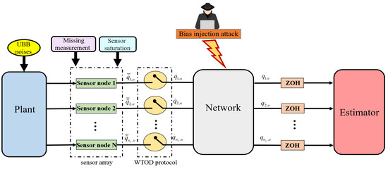
Figure 2. Schematic diagram of measurement saturation, MMs, WTOD protocol and cyber-attacks.

As shown in Figure 2, MMs can prevent the sensor from sending data to the network, which means that the network will not receive any information from this sensor if the MMs occur in this sensor. Hence, the measurement data that sent by sensors during MMs occur can be expressed as:

$${\overline{\tilde{q}}}_u={\alpha }_u{\tilde{q}}_u,$$

(9)

where ${\alpha }_u=\mathrm{diag}\{{\alpha }_u^1,{\alpha }_u^2,...,{\alpha }_u^{n_y}\}$ is the known matrix, ${\alpha }_u^i\in \{0,1\}$ is used to indicate whether the MM occurs in the i-th sensor at sampling instant u, ${\alpha }_u^i=0$ represents the occurrence of the MM at sampling instant u and, on the contrary, ${\alpha }_u^i=1$ represents that the MM does not occur at sampling instant u.

To alleviate data conflicts caused by limited communication network bandwidth, the WTOD protocol is utilized to schedule the communication between the estimator and the sensor, which only allows a sensor node to transmit the latest data to the estimator during each sampling instant. Zero-order-holders (ZOHs) are used to maintain the information transmitted from other nodes at the previous sampling instant to compensate the loss of real-time data. The node $l_u\in \{1,2,\cdots ,n_y\}$ that sends data to the network at sampling instant u is selected according to

$$l_u=arg\underset{1\le i\le n_y}{max}{({\overline{\tilde{q}}}_{i,u}-{\dot{q}}_{i,u-1})}^{\mathrm{T}}{\partial }_i({\overline{\tilde{q}}}_{i,u}-{\dot{q}}_{i,u-1}),$$

where ${\dot{q}}_{i,u-1}$ represents the latest data sent by the sensor node i before sampling instant u, and ${\partial }_i>0$ is a known matrix that represents the weight coefficient of the sensor node i. ${\dot{q}}_u={({\dot{q}}_{1,u},{\dot{q}}_{2,u},\cdots ,{\dot{q}}_{n_y,u})}^{\mathrm{T}}$ represents the actual output after the output of the sensors are scheduled by the WTOD protocol, and the update rule for ${\dot{q}}_{i,u}$ $(u\in N^{+},i\in n_y)$ can be formulated as

$${\dot{q}}_{i,u}=\left\{\begin{array}{c}{\overline{\tilde{q}}}_{i,u} i=l_u\hfill \\ {\dot{q}}_{i,u-1} i\ne l_u\hfill \end{array}\right.$$

Define $\Xi \left(l_u\right)=\mathrm{diag}\{{\Re }_{1-l_u},{\Re }_{2-l_u},\cdots ,{\Re }_{n_y-l_u}\}$; then, $q_u$ can be rewritten as

$${\dot{q}}_u={\Xi }_{l_u}{\overline{\tilde{q}}}_u+(1-{\Xi }_{l_u}){\dot{q}}_{u-1},$$

(10)

where ${\Re }_{i-l_u}\in \left\{01\right\}$ is the Kronecker delta function.

Remark 1.

During the state estimation of MNNs, the sensors send data to the estimator using communication networks at each sampling instant. Nevertheless, the transmission capacity of the network is typically constrained in practical scenarios, which causes network-induced phenomena such as transmission delay or out-of-order. To reduce the occurrence of these phenomena, utilizing the WTOD protocol to reduce the number of data packets transmitted is important. The process of using the WTOD protocol to select sensor nodes is divided into two stages at each instant: the initial stage is to calculate the difference between ${\overline{\tilde{q}}}_{i,u}$ and ${\dot{q}}_{i,u-1}$, and the subsequent stage is to prioritize the nodes through combining the established weight coefficients and the maximal difference acquired during the initial stage. Noteworthy is the fact that the node which has that smallest number of indexes is usually selected when multiple nodes have the same priority.

As one of the most destructive cyber-attacks, bias injection attack refers to the malicious injection of an attack signal into the measurement data transmitted to the estimator, which makes the estimator receive false information. Hence, the measurement data that are subject to cyber-attacks received by the estimator can be expressed as

$$q_u={\dot{q}}_u+{\beta }_u{\Xi }_{l_u}{\rho }_u,$$

(11)

where ${\beta }_u\in \{0,1\}$ is used to indicate whether the bias injection attack occurs at sampling instant u, in which ${\beta }_u=1$ represents the occurrence of the bias injection attack at sampling instant u and ${\beta }_u=0$ represents the networks that are not subject to the bias injection attack at sampling instant u. ${\rho }_u$ represents the signal of bias injection attack and satisfies the following assumption:

$$\mathrm{E}\left\{{\rho }_u^{\mathrm{T}}{\Omega }_u^{-1}{\rho }_u\right\}\le 1,$$

(12)

where ${\Omega }_u$ is a known scaled positive definite matrix.

To reflect engineering practice better, we assume that the MM is persistent, while the bias injection attack occurs stochastically and follows the Bernoulli distribution:

$$\mathrm{P}\{{\beta }_u=1\}=\overline{\tilde{\beta }},\mathrm{P}\{{\beta }_u=0\}=1-\overline{\tilde{\beta }},$$

where $\overline{\tilde{\beta }}\in [0,1)$ is a known constant.

Let $o_u={\left({\overline{\tilde{o}}}_u^{\mathrm{T}}{\dot{q}}_{u-1}^{\mathrm{T}}\right)}^{\mathrm{T}}$; then, the augmented form of measurement saturated-MNNs, with MMs and mixed time delays subject to cyber-attacks under the framework of WTOD protocol, can be expressed in the following:

$$\left\{\begin{array}{c}{o}_{u+1}={\aleph }_{u}A\left(o_u\right)o_u+B\left(o_u\right)F\left(o_u\right)+D\left(o_u\right)G\left(o_{u-{\tau }_1}\right)+E\left(o_u\right)\sum _{i=1}^{{\tau }_2}{\mu }_i{o}_{u-i}\hfill \\ +{\aleph }_u{H}_1{W}_u+{\alpha }_u{I}_u\theta \left(C_1{o}_u\right)\hfill \\ q_u={\alpha }_u{C}_2{o}_u+{\alpha }_u{\Xi }_{l_u}\theta \left(C_1{o}_u\right)+{\alpha }_u{H}_2{W}_u+{\beta }_u{\Xi }_{l_u}{\rho }_u\hfill \\ o_u={\Psi }_u,u\in [-\tau ,0]\hfill \end{array}\right.$$

(13)

where

$${\aleph }_u=\left(\begin{array}{cc}I& 0\\ 0& {\alpha }_u\end{array}\right),A\left(o_u\right)=\left(\begin{array}{cc}\overline{\tilde{A}}\left({\overline{\tilde{o}}}_u\right)& 0\\ {\Xi }_{l_u}{\overline{\tilde{U}}}_1\overline{\tilde{C}}& I-{\Xi }_{l_u}\end{array}\right),$$

$$B\left(o_u\right)=\left(\begin{array}{cc}\overline{\tilde{B}}\left({\overline{\tilde{o}}}_u\right)& 0\\ 0& 0\end{array}\right),F\left(o_u\right)=\left(\begin{array}{c}f\left({\overline{\tilde{o}}}_u\right)\hfill \\ 0\hfill \end{array}\right),$$

$$D\left(o_u\right)=\left(\begin{array}{cc}\overline{\tilde{D}}\left({\overline{\tilde{o}}}_u\right)& 0\\ 0& 0\end{array}\right),G\left(o_{u-{\tau }_1}\right)=\left(\begin{array}{c}g\left({\overline{\tilde{o}}}_{u-{\tau }_1}\right)\hfill \\ 0\hfill \end{array}\right),$$

$$E\left(o_u\right)=\left(\begin{array}{cc}\overline{\tilde{E}}\left({\overline{\tilde{o}}}_u\right)& 0\\ 0& 0\end{array}\right),H_1=\left(\begin{array}{cc}{\overline{\tilde{H}}}_w& 0\\ 0& {\Xi }_{l_u}{\overline{\tilde{H}}}_v\end{array}\right),$$

$$W_u=\left(\begin{array}{c}{\overline{\tilde{W}}}_u\hfill \\ {\overline{\tilde{V}}}_u\hfill \end{array}\right),C_1=\left(\begin{array}{cc}\overline{\tilde{C}}& 0\end{array}\right),C_2=\left(\begin{array}{cc}{\Xi }_{l_u}{\overline{\tilde{U}}}_1\overline{\tilde{C}}& I-{\Xi }_{l_u}\end{array}\right),$$

$$I_u=\left(\begin{array}{cc}0& {\Xi }_{l_u}\end{array}\right),H_2=\left(0\left.{\Xi }_{l_u}{\overline{\tilde{H}}}_v\right).\right.$$

and ${\Psi }_u$ is the augmented initial value.

By separating unknown matrices $\Delta {\overline{\tilde{A}}}_u$, $\Delta {\overline{\tilde{B}}}_u$, $\Delta {\overline{\tilde{D}}}_u$ and $\Delta {\overline{\tilde{E}}}_u$, the matrices $A\left(o_u\right)$, $B\left(o_u\right)$, $D\left(o_u\right)$ and $E\left(o_u\right)$ can be decomposed into the following expressions:

$$A\left(o_u\right)=A+\Delta A_u,B\left(o_u\right)=B+\Delta B_u,$$

$$D\left(o_u\right)=D+\Delta D_u,E\left(o_u\right)=E+\Delta E_u,$$

where

$$A=\left(\begin{array}{cc}\overline{\tilde{A}}& 0\\ {\Xi }_{l_u}{\overline{\tilde{U}}}_1\overline{\tilde{C}}& I-{\Xi }_{l_u}\end{array}\right),\Delta A_u=\left(\begin{array}{cc}\Delta {\overline{\tilde{A}}}_u& 0\\ 0& 0\end{array}\right),$$

$$B=\left(\begin{array}{cc}\overline{\tilde{B}}& 0\\ 0& 0\end{array}\right),\Delta B_u=\left(\begin{array}{cc}\Delta {\overline{\tilde{B}}}_u& 0\\ 0& 0\end{array}\right),D=\left(\begin{array}{cc}\overline{\tilde{D}}& 0\\ 0& 0\end{array}\right),$$

$$\Delta D_u=\left(\begin{array}{cc}\Delta {\overline{\tilde{D}}}_u& 0\\ 0& 0\end{array}\right),E=\left(\begin{array}{cc}\overline{\tilde{E}}& 0\\ 0& 0\end{array}\right),\Delta E_u=\left(\begin{array}{cc}\Delta {\overline{\tilde{E}}}_u& 0\\ 0& 0\end{array}\right).$$

According to (8), the unknown parameter matrices $\Delta A_u$, $\Delta B_u$, $\Delta D_u$ and $\Delta E_u$ can be expressed with the following augmented form:

$$\begin{array}{cc}\hfill & \Delta A_u=T{\dot{F}}_{1,u}{X}_1,\Delta B_u=T{\dot{F}}_{2,u}{X}_2,\hfill \\ \hfill & \Delta D_u=T{\dot{F}}_{3,u}{X}_3,\Delta E_u=T{\dot{F}}_{4,u}{X}_4,\hfill \end{array}$$

(14)

where $T={\left(\begin{array}{cc}\overline{\tilde{T}}& 0\end{array}\right)}^{\mathrm{T}}$, $X_1=\left({\overline{\tilde{X}}}_{1}0\right)$, $X_2=\left({\overline{\tilde{X}}}_{2}0\right)$, $X_3=\left({\overline{\tilde{X}}}_{3}0\right)$, $X_4=\left({\overline{\tilde{X}}}_{4}0\right)$ and matrix ${\dot{F}}_u$ satisfies ${\dot{F}}_u^{\mathrm{T}}{\dot{F}}_u\le I$.

In summary, taking into account the effects of the gain perturbation of the estimator, cyber-attacks, mixed time delays, measurement saturation and MMs in the MNNs, the following estimator is designed:

$$\begin{array}{cc}\hfill & K_{u,n}=K_u+\Delta K_u\hfill \\ \hfill & {\widehat{o}}_{u+1}=A{\widehat{o}}_u+BF\left({\widehat{o}}_u\right)+DG\left({\widehat{o}}_{u-{\tau }_1}\right)+E\sum _{i=1}^{{\tau }_2}{\mu }_i{\widehat{o}}_{u-i}+K_{u,n}(q_u-{\alpha }_u{C}_2{\widehat{o}}_u)\hfill \end{array}$$

(15)

where ${\widehat{o}}_u\in {\mathrm{R}}^{n_y+n_x}$ is the estimated value of $o_u$, the matrix $K_u$ is the gain of estimator to be determined and $\Delta K_u$ is the gain perturbation of estimator satisfying

$$\Delta K_u=\widehat{T}{\widehat{F}}_u\widehat{X},$$

(16)

where ${\widehat{F}}_u$ is an unknown time-varying matrix satisfying ${\widehat{F}}_u^{\mathrm{T}}{\widehat{F}}_u\le 1$; $\widehat{T}$ and $\widehat{X}$ are known real matrices.

Remark 2.

During the process of state estimation, the system may encounter some issues such as actuator degradation, numerical calculation errors and the aging of components, which can cause gain perturbations in the estimator. In engineering practice, even small gain perturbations in the estimator can also lead to decreases in estimation performance. Consequently, researchers have devised non-fragile techniques to enhance the robustness of the estimator. As we all know, non-fragile technologies are mainly implemented through LMI. Noteworthy is the fact that the structure of LMI is changed when the MNNs are subjected to the stochastic cyber-attacks, so the traditional non-fragile estimation framework based on SMF is no longer applicable. To solve this issue, this paper designs a new non-fragile set-membership estimation framework by adjusting the structure of the matrices $\tilde{T}$ and $\tilde{X}$ correspondingly, based on Lemma 3 in the following derivation.

Assumption 2.

The initial values ${\Psi }_i$ $(i\in [-\tau ,0\left]\right)$ belong to the ellipsoid sets given below:

$$z_i=\{{\Psi }_i\in {\mathrm{R}}^{n_x+n_y}:{\Psi }_i^T{P}_i^{-1}{\Psi }_i\le 1\},$$

(17)

where $P_i$$(i\in [-\tau ,0\left]\right)$ are known positive definite matrices.

The primary aim of this paper is to design a new non-fragile set-membership estimator to estimate the state of measurement-saturated MNNs with MMs and mixed time delays subject to cyber-attacks under the framework of the WTOD protocol, which mainly includes the following two parts:

(1) Obtain the estimator gain matrices $K_u$ such that the positive definite matrices $P_{u+1}$ and ${\widehat{o}}_{u+1}$ satisfy the constraints of the ellipsoid sets as follows:

$$\begin{array}{cc}\hfill & z_{u+1}=\{o_{u+1}\in {\mathrm{R}}^{n_x+n_y}:\hfill \\ \hfill & {(o_{u+1}-{\widehat{o}}_{u+1})}^{\mathrm{T}}{P}_{u+1}^{-1}(o_{u+1}-{\widehat{o}}_{u+1})\le 1\};\hfill \end{array}$$

(18)

(2) Design an optimization algorithm by minimizing the trace of $P_{u+1}$ to achieve local optimal estimation performance.

To facilitate subsequent derivation, some lemmas are introduced as follows.

Lemma 1

([61]). Given constant matrices ${\tilde{\wp }}_1$, ${\tilde{\wp }}_2$ and ${\tilde{\wp }}_3$ satisfying ${\tilde{\wp }}_1={\tilde{\wp }}_1^T$, ${\tilde{\wp }}_2={\tilde{\wp }}_2^T>0$, then

$${\tilde{\wp }}_1+{\tilde{\wp }}_3^T{\tilde{\wp }}_2^{-1}{\tilde{\wp }}_3<0,$$

if and only if

$$\left(\begin{array}{cc}{\tilde{\wp }}_1& {\tilde{\wp }}_3^T\\ {\tilde{\wp }}_3& -{\tilde{\wp }}_2\end{array}\right)<0,\left(\begin{array}{cc}-{\tilde{\wp }}_2& {\tilde{\wp }}_3\\ {\tilde{\wp }}_3^T& {\tilde{\wp }}_1\end{array}\right)<0.$$

Lemma 2

([61]). Let $q_i(\perp )$ $(i=0,1,2,\cdots ,t)$ be quadratic functions of the variable $\perp \in R^{n_x}$, that is, $q_i(\perp )={\perp }^T{p}_i\perp$, where

$${p_i}^T=p_i.$$

If there exists ${\nabla }_i>0$ $(i=0,1,2,\cdots ,t)$ satisfying $p_0-{\displaystyle \sum _{i=1}^t}{\nabla }_i{p}_i\le 0$, then, one has

$$q_1(\perp )\le 0,q_2(\perp )\le 0,\cdots ,q_p(\perp )\le 0\Rightarrow q_0(\perp )\le 0.$$

Lemma 3

([61]). Given matrices $\gamma ={\gamma }^{\mathrm{T}}$, T and X, which are real matrices with appropriate dimensions, the following inequality:

$$\gamma +T{F}_{u}X+X^T{F_u}^T{T}^T<0,$$

holds, for all $F_u$ satisfying ${F_u}^T{F}_u\le 1$, if and only if there exists a positive scalar $\iota >0$ satisfying

$$\gamma +{\iota }^{-1}T{T}^{\mathrm{T}}+\iota X^{\mathrm{T}}X<0.$$

3. Main Result

3.1. Estimator Design

The subsequent theorem gives the sufficient conditions for constraining estimation error within desired ellipsoidal regions by employing the LMI approach.

Theorem 1.

Considering the augmented MNNs in (13) and the estimator in (15), the estimation error can still be constrained within the required ellipsoidal region at the sampling instant $u+1$ if there is a set of real matrices $P_{u+1}>0$, $K_u$, positive scalars ${\phi }_j$ $(j=1,2,\cdots ,n_y)$, ${϶}_i$ $(i=1,2,\cdots ,8)$ and $\iota$ that satisfy the following LMI:

$$\gamma =\left(\begin{array}{ccc}\tilde{\gamma }& \tilde{T}& \iota {\tilde{X}}^T\\ \ast & -\iota I& 0\\ \ast & \ast & -\iota I\end{array}\right)\le 0,$$

(19)

where

$$\begin{array}{c}\tilde{\gamma }=\left(\begin{array}{cc}-P_{u+1}& {\stackrel{\rightharpoonup }{\epsilon }}_u\\ \ast & {\Lambda }_u\end{array}\right),\hfill \\ {\epsilon }_u={\stackrel{\leftharpoonup }{\epsilon }}_u+{\stackrel{\rightharpoonup }{\epsilon }}_u,\hfill \\ \left(\begin{array}{cc}-P_{u+1}& {\epsilon }_u\\ \ast & {\Lambda }_u\end{array}\right)=\left(\begin{array}{cc}-P_{u+1}& {\stackrel{\rightharpoonup }{\epsilon }}_u\\ \ast & {\Lambda }_u\end{array}\right)+\left(\begin{array}{cc}0& {\stackrel{\leftharpoonup }{\epsilon }}_u\\ \ast & 0\end{array}\right),\hfill \\ {\stackrel{\leftharpoonup }{\epsilon }}_u={\stackrel{\leftharpoonup }{\epsilon }}_u^1+{\stackrel{\leftharpoonup }{\epsilon }}_u^2,{\stackrel{\leftharpoonup }{\epsilon }}_u=\left(\begin{array}{cc}{\dot{\stackrel{\leftharpoonup }{\epsilon }}}_u& {\ddot{\stackrel{\leftharpoonup }{\epsilon }}}_u\end{array}\right),\hfill \\ {\dot{\stackrel{\leftharpoonup }{\epsilon }}}_u=\left(\begin{array}{ccccc}{\stackrel{\leftharpoonup }{\epsilon }}_{1,u}& {\stackrel{\leftharpoonup }{\epsilon }}_{2,u}& 0& \Delta E_u{\displaystyle \sum _{i=1}^{{\tau }_2}}{\mu }_i{L}_{u-i}& \Delta D_u\\ 0& 0& 0& 0& 0\end{array}\right),\hfill \\ {\ddot{\stackrel{\leftharpoonup }{\epsilon }}}_u=\left(\begin{array}{cccc}{\stackrel{\leftharpoonup }{\epsilon }}_{3,u}& {\stackrel{\leftharpoonup }{\epsilon }}_{4,u}& {\stackrel{\leftharpoonup }{\epsilon }}_{5,u}^1& \Delta B_u\\ 0& 0& {\stackrel{⌣}{\stackrel{\leftharpoonup }{\epsilon }}}_{5,u}^2& 0\end{array}\right),\hfill \\ {\stackrel{\leftharpoonup }{\epsilon }}_{1,u}=\Delta A_u{\widehat{o}}_u+\Delta E_u\sum _{i=1}^{{\tau }_2}{\mu }_i{\widehat{o}}_{u-i},\hfill \\ {\stackrel{\leftharpoonup }{\epsilon }}_{2,u}=(\Delta A_u-{\alpha }_u\Delta K_u{C}_2)L_u,\hfill \\ {\stackrel{\leftharpoonup }{\epsilon }}_{3,u}=-{\alpha }_u\Delta K_u{\Xi }_{l_u},{\stackrel{\leftharpoonup }{\epsilon }}_{4,u}=-{\alpha }_u\Delta K_u{H}_2,\hfill \\ {\stackrel{\leftharpoonup }{\epsilon }}_{5,u}^1=-\overline{\tilde{\beta }}\Delta K_u{\Xi }_{l_u},{\stackrel{⌣}{\stackrel{\leftharpoonup }{\epsilon }}}_{5,u}^2=-{\stackrel{⌣}{\beta }}_u\Delta K_u{\Xi }_{l_u},\hfill \\ {\Lambda }_u={\Lambda }_{1u}+{\Lambda }_{2u},\hfill \\ {\Lambda }_{1u}=\mathrm{diag}\{{\Lambda }_{11u},-{϶}_{1}I,-{϶}_{2}I,-{϶}_{3}I,\hfill \\ 0,0,-{϶}_4{R_u}^{-1},-{϶}_5{\Omega }_u^{-1},0\},\hfill \\ {\Lambda }_{11u}=-1+{϶}_1+{϶}_2+{\tau }_2{϶}_3+2{϶}_4+{϶}_5,\hfill \\ {\Lambda }_{2u}=-{϶}_8{Y}_u-{϶}_7{\pi }_u-{϶}_6{\xi }_u-\sum _{j=1}^{n_y}{\phi }_j{Q}_u^T\tilde{\omega }({\Xi }_j-{\Xi }_{l_u})Q_u,\hfill \\ {\stackrel{\rightharpoonup }{\epsilon }}_u=\left(\begin{array}{cc}\dot{\stackrel{\rightharpoonup }{\epsilon }}& \ddot{\stackrel{\rightharpoonup }{\epsilon }}\end{array}\right),\hfill \\ \dot{\stackrel{\rightharpoonup }{\epsilon }}=\left(\begin{array}{cccc}{\stackrel{\rightharpoonup }{\epsilon }}_{1,u}& {\stackrel{\rightharpoonup }{\epsilon }}_{2,u}& 0& E\left(o_u\right){\displaystyle \sum _{i=1}^{{\tau }_2}}{\mu }_i{o}_{u-i}\\ 0& 0& 0& 0\end{array}\right),\hfill \\ \ddot{\stackrel{\rightharpoonup }{\epsilon }}=\left(\begin{array}{ccccc}D\left(o_u\right)& {\stackrel{\rightharpoonup }{\epsilon }}_{3,u}& {\stackrel{\rightharpoonup }{\epsilon }}_{4,u}& {\stackrel{\rightharpoonup }{\epsilon }}_{5,u}^1& B\left(o_u\right)\\ 0& 0& 0& {\stackrel{⌣}{\stackrel{\rightharpoonup }{\epsilon }}}_{5,u}^2& 0\end{array}\right),\hfill \\ {\stackrel{\rightharpoonup }{\epsilon }}_{1,u}=-BF\left({\widehat{o}}_u\right)-DG\left({\widehat{o}}_{u-{\tau }_1}\right),\hfill \\ {\stackrel{\rightharpoonup }{\epsilon }}_{2,u}=\left({\aleph }_{u}A\left(o_u\right)-{\alpha }_u{K}_u{C}_2\right)L_u,\hfill \\ {\stackrel{\rightharpoonup }{\epsilon }}_{3,u}={\alpha }_u{I}_u-{\alpha }_u{K}_u{\Xi }_{l_u},{\stackrel{\rightharpoonup }{\epsilon }}_{4,u}={\aleph }_u{H}_1-{\alpha }_u{K}_u{H}_2,\hfill \\ {\stackrel{\rightharpoonup }{\epsilon }}_{5,u}^1=-\overline{\tilde{\beta }}{K}_u{\Xi }_{l_u},{\stackrel{⌣}{\stackrel{\rightharpoonup }{\epsilon }}}_{5,u}^2=-{\stackrel{⌣}{\beta }}_u{K}_u{\Xi }_{l_u},{\stackrel{⌣}{\beta }}_u=\sqrt{\overline{\tilde{\beta }}(1-\overline{\tilde{\beta }})},\hfill \end{array}$$

$$\begin{array}{c}\tilde{T}={\left(\begin{array}{cccccccccc}{T}^T& 0& 0& 0& 0& 0& 0& 0& 0& 0\end{array}\right)}^{\mathrm{T}},\hfill \\ T=\left(\begin{array}{cccccc}T& T& T& T& \widehat{T}& 0\\ 0& 0& 0& 0& 0& \widehat{T}\end{array}\right),\tilde{X}=\left(\begin{array}{cc}0& X\end{array}\right),\hfill \\ X=\left(\begin{array}{cc}{X}_{11}& X_{12}\\ X_{21}& X_{22}\end{array}\right),X_{11}=\left(\begin{array}{cccc}{X}_1{\widehat{o}}_u& X_1{L}_u& 0& 0\\ 0& 0& 0& 0\\ 0& 0& 0& 0\end{array}\right),\hfill \\ X_{21}=\left(\begin{array}{cccc}{X}_4{\displaystyle \sum _{i=1}^{{\tau }_2}}{\mu }_i{\widehat{o}}_{u-i}& 0& 0& X_4{\displaystyle \sum _{i=1}^{{\tau }_2}}{\mu }_i{L}_{u-i}\\ 0& -{\alpha }_u\widehat{X}{C}_2{L}_u& 0& 0\\ 0& 0& 0& 0\end{array}\right),\hfill \\ X_{12}=\left(\begin{array}{ccccc}0& 0& 0& 0& 0\\ 0& 0& 0& 0& X_2\\ X_3& 0& 0& 0& 0\end{array}\right),X_{22}=\left(\begin{array}{ccccc}0& 0& 0& 0& 0\\ 0& -{\alpha }_u\widehat{X}{\Xi }_{l_u}& -{\alpha }_u\widehat{X}{H}_2& -\overline{\tilde{\beta }}\widehat{X}{\Xi }_{l_u}& 0\\ 0& 0& 0& -{\beta }_u\widehat{X}{\Xi }_{l_u}& 0\end{array}\right),\hfill \end{array}$$

(20)

in which $L_u$ is a Cholesky factorization of $P_u=L_u{L}_u^{\mathrm{T}}$.

Proof. 

The mathematical induction is introduced to prove Theorem 1. First, we can know that ${(o_0-{\widehat{o}}_0)}^{\mathrm{T}}{P}_0^{-1}(o_0-{\widehat{o}}_0)\le 1$ from Assumption 2 when the sampling instant $u=0$. Next, we assume that ${(o_u-{\widehat{o}}_u)}^{\mathrm{T}}{P}_u^{-1}(o_u-{\widehat{o}}_u)\le 1$ holds when the sampling instant $u\ge 0$. Finally, we need to prove that ${(o_{u+1}-{\widehat{o}}_{u+1})}^{\mathrm{T}}{P}_{u+1}^{-1}$$(o_{u+1}-{\widehat{o}}_{u+1})\le 1$ also holds when the sampling instant $u+1\ge 0$. The proof process is shown as follows.

As mentioned in [62], there exists a vector $M_u$ with $∥M_u∥\le 1$ satisfying

$$e_u=o_u-{\widehat{o}}_u=L_u{M}_u,$$

(21)

where $L_u$ is given in (20). Therefore, the estimation error can be obtained by the process of calculation as follows:

$$\begin{array}{cc}\hfill & o_{u+1}-{\widehat{o}}_{u+1}\hfill \\ \hfill & ={\aleph }_{u}A\left(o_u\right)o_u+B\left(o_u\right)F\left(o_u\right)+D\left(o_u\right)G\left(o_{u-{\tau }_1}\right)\hfill \\ \hfill & +E\left(o_u\right)\sum _{i=1}^{{\tau }_2}{\mu }_i{o}_{u-i}+{\aleph }_u{H}_1{W}_u+{\alpha }_u{I}_{1u}\theta \left(C_1{o}_u\right)\hfill \\ \hfill & -{\aleph }_{u}A{\widehat{o}}_u-BF\left({\widehat{o}}_u\right)-DG\left({\widehat{o}}_{u-{\tau }_1}\right)-E\sum _{i=1}^{{\tau }_2}{\mu }_i{\widehat{o}}_{u-i}\hfill \\ \hfill & +(K_u+\Delta K_u)(q_u-{\alpha }_u{C}_2{\widehat{o}}_u)\hfill \\ \hfill & ={\aleph }_{u}A\left(o_u\right)e_u+\Delta A_u{\widehat{o}}_u+B\left(o_u\right)F\left({\widehat{o}}_u\right)\hfill \\ \hfill & -BF\left({\widehat{o}}_u\right)+D\left(o_u\right)G\left(o_{u-{\tau }_1}\right)-DG\left({\widehat{o}}_{u-{\tau }_1}\right)\hfill \\ \hfill & +E\left(o_u\right)\sum _{i=1}^{{\tau }_2}{\mu }_i{e}_{u-i}+\Delta E_u\sum _{i=1}^{{\tau }_2}{\mu }_i{\widehat{o}}_{u-i}\hfill \\ \hfill & +({\aleph }_u{H}_1-{\alpha }_u(\Delta K_u+K_u)H_2)W_u\hfill \\ \hfill & +({\alpha }_u{I}_u-{\alpha }_u(\Delta K_u+K_u){\Xi }_{l_u})\theta \left(C_1{o}_u\right)\hfill \\ \hfill & -{\beta }_u(\Delta K_u+K_u){\Xi }_{l_u}{\rho }_u-{\alpha }_u(\Delta K_u+K_u)C_2{e}_u.\hfill \end{array}$$

(22)

For convenience, the following notations are defined:

$$\begin{array}{c}{y}_u={\left(\begin{array}{cc}{\dot{y}}_u& {\ddot{y}}_u\end{array}\right)}^{\mathrm{T}},\hfill \\ {\dot{y}}_u=\left(\begin{array}{ccccc}1& M_u^{\mathrm{T}}& M_{u-{\tau }_1}^{\mathrm{T}}& M_{\tau u}^{\mathrm{T}}& G^{\mathrm{T}}\left(o_{u-{\tau }_1}\right)\end{array}\right),\hfill \\ {\ddot{y}}_u=\left(\begin{array}{cccc}{\theta }^{\mathrm{T}}\left(C_1{o}_u\right)& W_u^{\mathrm{T}}& {\rho }_u^{\mathrm{T}}& F^{\mathrm{T}}\left(o_u\right)\end{array}\right),\hfill \\ M_{\tau u}={\left(\begin{array}{cccc}{M}_{u-1}^{\mathrm{T}}& M_{u-2}^{\mathrm{T}}& \cdots & M_{u-{\tau }_2}^{\mathrm{T}}\end{array}\right)}^{\mathrm{T}}.\hfill \end{array}$$

(23)

Then, the estimation error can be rewritten as the below compact form:

$$o_{u+1}-{\widehat{o}}_{u+1}={\epsilon }_u{y}_u,$$

(24)

where

$$\begin{array}{c}{\epsilon }_u=\left(\begin{array}{cc}{\dot{\epsilon }}_u& {\ddot{\epsilon }}_u\end{array}\right),\hfill \\ {\dot{\epsilon }}_u=\left(\begin{array}{ccccc}{\epsilon }_{1,u}& {\epsilon }_{2,u}& 0& E\left(o_u\right){\displaystyle \sum _{i=1}^{{\tau }_2}}{\mu }_i{L}_{u-i}& D\left(o_u\right)\end{array}\right),\hfill \\ {\ddot{\epsilon }}_u=\left(\begin{array}{cccc}{\epsilon }_{3,u}& {\epsilon }_{4,u}& {\epsilon }_{5,u}& B\left(o_u\right)\end{array}\right),\hfill \\ {\epsilon }_{1,u}=\Delta A_u{\widehat{o}}_u-BF\left({\widehat{o}}_u\right)-DG\left({\widehat{o}}_{u-{\tau }_1}\right)+\Delta E_u{\displaystyle \sum _{i=1}^{{\tau }_2}}{\mu }_i{\widehat{o}}_{u-i},\hfill \\ {\epsilon }_{2,u}=({\aleph }_{u}A\left(o_u\right)-{\alpha }_u(\Delta K_u+K_u)C_2)L_u,\hfill \\ {\epsilon }_{3,u}={\alpha }_u{I}_u-{\alpha }_u(\Delta K_u+K_u){\Xi }_{l_u},\hfill \\ {\epsilon }_{4,u}={\aleph }_u{H}_1-{\alpha }_u(\Delta K_u+K_u)H_2,\hfill \\ {\epsilon }_{5,u}=-{\beta }_u(\Delta K_u+K_u){\Xi }_{l_u}.\hfill \end{array}$$

Next, the stochastic matrix ${\epsilon }_u$ can be decomposed through a specific process:

$${\epsilon }_u={\epsilon }_u^1+{\epsilon }_u^2,$$

(25)

where

$$\begin{array}{c}{\epsilon }_u^1=\left(\begin{array}{cc}{\dot{\epsilon }}_u^1& {\ddot{\epsilon }}_u^1\end{array}\right),\hfill \\ {\dot{\epsilon }}_u^1=\left(\begin{array}{ccccc}{\epsilon }_{1,u}& {\epsilon }_{2,u}& 0& E\left(o_u\right){\displaystyle \sum _{i=1}^{{\tau }_2}}{\mu }_i{L}_{u-i}& D\left(o_u\right)\end{array}\right),\hfill \\ {\ddot{\epsilon }}_u^1=\left(\begin{array}{cccc}{\epsilon }_{3,u}& {\epsilon }_{4,u}& {\epsilon }_{5,u}^1& B\left(o_u\right)\end{array}\right),\hfill \\ {\epsilon }_{5,u}^1=-\overline{\tilde{\beta }}(\Delta K_u+K_u){\Xi }_{l_u},\hfill \\ {\epsilon }_u^2=\left(\begin{array}{ccccccccc}0& 0& 0& 0& 0& 0& 0& {\epsilon }_{5,u}^2& 0\end{array}\right),\hfill \\ {\epsilon }_{5,u}^2=-{\tilde{\beta }}_u(\Delta K_u+K_u){\Xi }_{l_u},\hfill \\ {\beta }_u=\overline{\tilde{\beta }}+{\tilde{\beta }}_u,\hfill \end{array}$$

Subsequently, $y_u^{\mathrm{T}}{\epsilon }_u^{\mathrm{T}}{P}_{u+1}^{-1}{\epsilon }_u{y}_u$ can be rewritten as a new form:

$$\begin{array}{c}{y}_u^{\mathrm{T}}{\epsilon }_u^{\mathrm{T}}{P}_{u+1}^{-1}{\epsilon }_u{y}_u\hfill \\ =y_u^{\mathrm{T}}({\epsilon }_u^{1\mathrm{T}}{P}_{u+1}^{-1}{\epsilon }_u^1+{\epsilon }_u^{2\mathrm{T}}{P}_{u+1}^{-1}{\epsilon }_u^2)y_u\hfill \\ =y_u^{\mathrm{T}}{\Im }_u{y}_u.\hfill \end{array}$$

(26)

Therefore, $y_u^{\mathrm{T}}{\epsilon }_u^{\mathrm{T}}{P}_{u+1}^{-1}{\epsilon }_u{y}_u\le 1$ can be rewritten as

$$y_u^{\mathrm{T}}\left({\Im }_u-\mathrm{diag}\{1,0,...,0\}\right)y_u\le 0.$$

(27)

According to inequalities (2) and (10), the following constraint conditions can be obtained:

$$\left\{\begin{array}{c}{∥M_u∥}^2\le 1\hfill \\ {∥M_{u-{\tau }_1}∥}^2\le 1\hfill \\ {∥M_{\tau u}∥}^2\le {\tau }_2\hfill \\ W_u^{\mathrm{T}}{R}_u^{-1}{W}_u\le 2\hfill \\ {\rho }_u^{\mathrm{T}}{\Omega }_u^{-1}{\rho }_u\le 1\hfill \end{array}\right.$$

(28)

which can be rewritten as

$$\left\{\begin{array}{c}{y}_u^{\mathrm{T}}\mathrm{diag}\{-1,I,0,...,0\}{y}_u\le 0\hfill \\ y_u^{\mathrm{T}}\mathrm{diag}\{-1,0,I,0,...,0\}{y}_u\le 0\hfill \\ y_u^{\mathrm{T}}\mathrm{diag}\{-{\tau }_2,0,0,I,0,...,0\}{y}_u\le 0\hfill \\ y_u^{\mathrm{T}}\mathrm{diag}\{-2,0,...,0,R_u^{-1},0,0\}{y}_u\le 0\hfill \\ y_u^{\mathrm{T}}\mathrm{diag}\{-1,0,...,0,{\Omega }_u^{-1},0\}{y}_u\le 0\hfill \end{array}\right.$$

(29)

According to Inequalities (5) and (7), one obtains

$$\left\{\begin{array}{c}{\left(F\left(o_u\right)-J_1{o}_u\right)}^{\mathrm{T}}\left(F\left(o_u\right)-J_2{o}_u\right)\le 0\hfill \\ {\left(G\left(o_{u-{\tau }_1}\right)-S_1{o}_{u-{\tau }_1}\right)}^{\mathrm{T}}\left(G\left(o_{u-{\tau }_1}\right)-S_2{o}_{u-{\tau }_1}\right)\le 0\hfill \\ {\theta }^{\mathrm{T}}\left(C_1{o}_u\right)\left(\theta \left(C_1{o}_u\right)-U_2{o}_u\right)\le 0\hfill \end{array}\right.$$

(30)

which can be further described as

$$\left\{\begin{array}{c}{y}_u^{\mathrm{T}}{Y}_u{y}_u\le 0\hfill \\ y_u^{\mathrm{T}}{\xi }_u{y}_u\le 0\hfill \\ y_u^{\mathrm{T}}{\pi }_u{y}_u\le 0\hfill \end{array}\right.$$

(31)

where

$$Y_u=\left(\begin{array}{ccc}{Y}_{1u}& 0& Y_{2u}\\ \ast & 0& 0\\ \ast & \ast & I\end{array}\right),Y_{1u}=\left(\begin{array}{cc}{\widehat{o}}_u^{\mathrm{T}}{\tilde{J}}_2{\widehat{o}}_u& {\widehat{o}}_u^{\mathrm{T}}{\tilde{J}}_2{L}_u\\ \ast & L_u^{\mathrm{T}}{\tilde{J}}_2{L}_u\end{array}\right),$$

$$Y_{2u}=\left(\begin{array}{c}-{\widehat{o}}_u^{\mathrm{T}}{\tilde{J}}_1^{\mathrm{T}}\\ -L_u^{\mathrm{T}}{\tilde{J}}_1^{\mathrm{T}}\end{array}\right),J_1=\left(\begin{array}{cc}{\overline{\tilde{J}}}_1& 0\\ 0& 0\end{array}\right),J_2=\left(\begin{array}{cc}{\overline{\tilde{J}}}_2& 0\\ 0& 0\end{array}\right),$$

$${\tilde{J}}_1=(J_1+J_2)/2,{\tilde{J}}_2=(J_1^{\mathrm{T}}{J}_2+J_2^{\mathrm{T}}{J}_1)/2,$$

$${\xi }_u=\left(\begin{array}{cccc}{\xi }_{1u}& 0& {\xi }_{2u}& 0\\ \ast & 0& 0& 0\\ \ast & \ast & I& 0\\ \ast & \ast & \ast & 0\end{array}\right),{\xi }_{1u}=\left(\begin{array}{ccc}{\widehat{o}}_{u-{\tau }_1}^{\mathrm{T}}{\tilde{S}}_2{\widehat{o}}_{u-{\tau }_1}& 0& {\widehat{o}}_{u-{\tau }_1}^{\mathrm{T}}{\tilde{S}}_2{L}_{u-{\tau }_1}\\ \ast & 0& 0\\ \ast & \ast & L_{u-{\tau }_1}^{\mathrm{T}}{\tilde{S}}_2{L}_{u-{\tau }_1}\end{array}\right),$$

$${\xi }_{2u}=\left(\begin{array}{c}-{\widehat{o}}_{u-{\tau }_1}^{\mathrm{T}}{\tilde{S}}_1^{\mathrm{T}}\\ 0\\ -L_{u-{\tau }_1}^{\mathrm{T}}{\tilde{S}}_1^{\mathrm{T}}\end{array}\right),S_1=\left(\begin{array}{cc}{\overline{\tilde{S}}}_1& 0\\ 0& 0\end{array}\right),S_2=\left(\begin{array}{cc}{\overline{\tilde{S}}}_2& 0\\ 0& 0\end{array}\right),$$

$${\tilde{S}}_1=(S_1+S_2)/2,{\tilde{S}}_2=(S_1^{\mathrm{T}}{S}_2+S_2^{\mathrm{T}}{S}_1)/2,{\pi }_{1u}=\left(\begin{array}{c}-{\displaystyle \frac{1}{2}}{\widehat{o}}_u^{\mathrm{T}}{U}_2^{\mathrm{T}}\\ -{\displaystyle \frac{1}{2}}{L}_u^{\mathrm{T}}{U}_2^{\mathrm{T}}\end{array}\right),$$

$$U_2=\left(\begin{array}{cc}{\overline{\tilde{U}}}_2\overline{\tilde{C}}& 0\end{array}\right),{\pi }_u=\left(\begin{array}{cccccc}0& 0& {\pi }_{1u}& 0& 0& 0\\ \ast & 0& 0& 0& 0& 0\\ \ast & \ast & I& 0& 0& 0\\ \ast & \ast & \ast & 0& 0& 0\\ \ast & \ast & \ast & \ast & 0& 0\\ \ast & \ast & \ast & \ast & \ast & 0\end{array}\right).$$

Next, we can obtain the following formula from (10) that

$${({\overline{\tilde{q}}}_u-{\dot{q}}_{u-1})}^{\mathrm{T}}\tilde{\omega }({\Xi }_j-{\Xi }_{l_u})({\overline{\tilde{q}}}_u-{\dot{q}}_{u-1})\le 0,$$

(32)

where

$$\begin{array}{c}{\overline{\tilde{q}}}_u-{\dot{q}}_{u-1}\hfill \\ ={\alpha }_u{\overline{\tilde{U}}}_1\overline{\tilde{C}}{\overline{\tilde{o}}}_u+{\alpha }_u\theta \left(\overline{\tilde{C}}{\overline{\tilde{o}}}_u\right)+{\alpha }_u{\overline{\tilde{H}}}_v{\overline{\tilde{V}}}_u-{\dot{q}}_{u-1}\hfill \\ =C_3{o}_u+\theta \left(C_1{o}_u\right)+H_3{V}_u,\hfill \end{array}$$

$$C_3=\left({\alpha }_u\begin{array}{cc}{\overline{\tilde{U}}}_1\overline{\tilde{C}}& -I\end{array}\right),H_3=\left(\begin{array}{cc}0& {\alpha }_u{\overline{\tilde{H}}}_v\end{array}\right),{\overline{\tilde{q}}}_u-{\dot{q}}_{u-1}=Q_u{y}_u,$$

$$Q_u=\left(\begin{array}{ccccccccc}{C}_3{\widehat{o}}_u& C_3{L}_u& 0& 0& 0& {\alpha }_u& H_3& 0& 0\end{array}\right),$$

$$\tilde{\omega }=\mathrm{diag}\{{\omega }_1,{\omega }_2,\cdots ,{\omega }_{n_y}\}.$$

Inequality (32) is equivalent to

$$y_u^{\mathrm{T}}{Q}_u^{\mathrm{T}}\tilde{\omega }({\Xi }_j-{\Xi }_{l_u})Q_u{y}_u\le 0.$$

(33)

Based on Lemma 2, if there exist positive scalars ${϶}_i$ $(i=1,2,\cdots ,8)$ and ${\phi }_j$ $(j=1,2,\cdots ,n_y)$, such that

$$\begin{array}{cc}\hfill & {\Im }_u-{\kappa }_1-{϶}_1{\kappa }_2-{϶}_2{\kappa }_3-{϶}_3{\kappa }_4-{϶}_4{\kappa }_5-{϶}_5{\kappa }_6-{϶}_6{\xi }_u\hfill \\ \hfill & -{϶}_7{\pi }_u-{϶}_8{Y}_u-\sum _{j=1}^{n_y}{\phi }_j{Q}_u^{\mathrm{T}}\tilde{\omega }({\Xi }_j-{\Xi }_{l_u})Q_u\le 0,\hfill \end{array}$$

(34)

where

$$\begin{array}{c}{\kappa }_1=\mathrm{diag}\{1,0,...,0\},\hfill \\ {\kappa }_2=\mathrm{diag}\{-1,I,0,...,0\},\hfill \\ {\kappa }_3=\mathrm{diag}\{-1,0,I,0,...,0\},\hfill \\ {\kappa }_4=\mathrm{diag}\{-{\tau }_2,0,0,I,0,...,0\},\hfill \\ {\kappa }_5=\mathrm{diag}\{-2,0,...,0,R_u^{-1},0,0\},\hfill \\ {\kappa }_6=\mathrm{diag}\{-1,0,...,0,{\Omega }_u^{-1},0\},\hfill \end{array}$$

then the inequality (27) holds, and the following condensed form of Inequality (34) holds as well:

$${\Im }_u+{\Lambda }_u\le 0,$$

(35)

where ${\Lambda }_u$ is given in (20).

The following contents are used to handle the uncertainty of parameters and gain perturbations.

According to Lemma 1, the inequality (35) can be expressed as an LMI:

$$\left(\begin{array}{cc}-P_{u+1}& {\epsilon }_u\\ 0& {\Lambda }_u\end{array}\right)\le 0,$$

(36)

which can be decomposed into the following forms:

$$\tilde{\gamma }+\left(\begin{array}{cc}0& {\stackrel{\leftharpoonup }{\epsilon }}_u\\ \ast & 0\end{array}\right)\le 0,$$

(37)

where $\tilde{\gamma }$ and ${\stackrel{\leftharpoonup }{\epsilon }}_u$ are defined in (20). Then, the subsequent inequality can be derived by combining (14) and (16):

$$\tilde{\gamma }+\tilde{T}{\tilde{F}}_u\tilde{X}+{\tilde{X}}^{\mathrm{T}}{\tilde{F}}_u^{\mathrm{T}}{\tilde{T}}^{\mathrm{T}}<0,$$

(38)

where ${\tilde{F}}_u=\mathrm{diag}\left\{F_{1,u},F_{2,u},F_{3,u},F_{4,u},\widehat{F},\widehat{F}\right\}$, $\tilde{T}$ and $\tilde{X}$ are defined in (20).

Based on Lemma 3, there exists a positive scalar $\iota$ such that

$$\tilde{\gamma }+{\iota }^{-1}\tilde{T}{\tilde{T}}^{\mathrm{T}}+\iota {\tilde{X}}^{\mathrm{T}}\tilde{X}<0.$$

(39)

Then, we can derive from Lemma 3 that Equation (39) is equivalent to (19). The proof of Theorem 1 is ended. □

3.2. Optimization Problem

The estimator gain $K_u$ and the matrix $P_{u+1}>0$ that characterize the shape and direction of the ellipsoid are derived through iterative solutions of the sets of LMIs at each sampling instant. Noteworthy is the fact that, under the calculation framework discussed in the preceding sections, the obtained estimator gain $K_u$ could be a set (if existing). To determine the optimal estimator gain from this set, we propose a convex optimization problem: minimize the trace of the matrix $P_u$.

Corollary 1.

If there exist a series of real-valued matrices $P_{u+1}>0$ and $K_u$, positive scalars ${\phi }_j(j=1,2,\cdots ,n_y)$, ${϶}_i(i=1,2,\cdots ,8)$ and ι such that the following optimization problems can be solved:

$$\begin{array}{c}{\displaystyle \underset{\begin{array}{c}{P}_{u+1}>0,K_u,{϶}_i(i=1,2,\cdots ,8),\\ {\phi }_j(j=1,2,\cdots ,n_y),\iota \end{array}}{min}}\mathrm{trace}(P_{u+1})\\ \mathrm{if}\left(19\right)\mathrm{holds}\end{array}$$

(40)

then the minimized ellipsoidal regions can be obtained by minimizing the traces of the matrix $P_{u+1}$ sequence.

Remark 3.

In this paper, we consider multiple phenomena simultaneously, such as gain perturbation, cyber-attacks, time delays and MMs, which inevitably increase the complexity of the system to some extent. The added complexity may limit the applicability of the estimation framework in real-time systems with limited computational resources. However, we are considering the worst case here, and, in real situations, the considered phenomena occurring at the same time is not common—usually, only one of them occurs. These phenomena occurring in isolation are special cases under the framework of this paper. In this sense, the proposed estimation framework has little influence on the application in real-time systems with limited computational resources.

4. Simulation Example

In this section, we introduce a numerical example with parameters from [20] and an actual engineering example with parameters from [55] to verify the effectiveness of our designed approach.

Consider the MNN system in (13) with the following parameters:

$$a_1\left({\overline{\tilde{o}}}_{1,u}\right)=\left\{\begin{array}{c}0.84\left|{\overline{\tilde{o}}}_{1,u}\right|>1\hfill \\ 0.2\left|{\overline{\tilde{o}}}_{1,u}\right|\le 1\hfill \end{array},\right.a_2\left({\overline{\tilde{o}}}_{2,u}\right)=\left\{\begin{array}{c}0.35\left|{\overline{\tilde{o}}}_{2,u}\right|>1\hfill \\ 0.65\left|{\overline{\tilde{o}}}_{2,u}\right|\le 1\hfill \end{array},\right.$$

$$b_{11}\left({\overline{\tilde{o}}}_{1,u}\right)=\left\{\begin{array}{c}0.8\left|{\overline{\tilde{o}}}_{1,u}\right|>1\hfill \\ -0.2\left|{\overline{\tilde{o}}}_{1,u}\right|\le 1\hfill \end{array},\right.b_{12}\left({\overline{\tilde{o}}}_{1,u}\right)=\left\{\begin{array}{c}0.5\left|{\overline{\tilde{o}}}_{1,u}\right|>1\hfill \\ 0.7\left|{\overline{\tilde{o}}}_{1,u}\right|\le 1\hfill \end{array},\right.$$

$$b_{21}\left({\overline{\tilde{o}}}_{2,u}\right)=\left\{\begin{array}{c}-0.85\left|{\overline{\tilde{o}}}_{2,u}\right|>1\hfill \\ 0.05\left|{\overline{\tilde{o}}}_{2,u}\right|\le 1\hfill \end{array},\right.b_{22}\left({\overline{\tilde{o}}}_{2,u}\right)=\left\{\begin{array}{c}0.6\left|{\overline{\tilde{o}}}_{2,u}\right|>1\hfill \\ 0.8\left|{\overline{\tilde{o}}}_{2,u}\right|\le 1\hfill \end{array},\right.$$

$$d_{11}\left({\overline{\tilde{o}}}_{1,u}\right)=\left\{\begin{array}{c}0.2\left|{\overline{\tilde{o}}}_{1,u}\right|>1\hfill \\ 0.1\left|{\overline{\tilde{o}}}_{1,u}\right|\le 1\hfill \end{array},\right.d_{12}\left({\overline{\tilde{o}}}_{1,u}\right)=\left\{\begin{array}{c}-0.3\left|{\overline{\tilde{o}}}_{1,u}\right|>1\hfill \\ 0.12\left|{\overline{\tilde{o}}}_{1,u}\right|\le 1\hfill \end{array},\right.$$

$$d_{21}\left({\overline{\tilde{o}}}_{2,u}\right)=\left\{\begin{array}{c}0.5\left|{\overline{\tilde{o}}}_{2,u}\right|>1\hfill \\ -0.35\left|{\overline{\tilde{o}}}_{2,u}\right|\le 1\hfill \end{array},\right.d_{22}\left({\overline{\tilde{o}}}_{2,u}\right)=\left\{\begin{array}{c}0.1\left|{\overline{\tilde{o}}}_{2,u}\right|>1\hfill \\ 0.06\left|{\overline{\tilde{o}}}_{2,u}\right|\le 1\hfill \end{array},\right.$$

$$h_{11}\left({\overline{\tilde{o}}}_{1,u}\right)=\left\{\begin{array}{c}0.2\left|{\overline{\tilde{o}}}_{1,u}\right|>1\hfill \\ 0.1\left|{\overline{\tilde{o}}}_{1,u}\right|\le 1\hfill \end{array},\right.h_{12}\left({\overline{\tilde{o}}}_{1,u}\right)=\left\{\begin{array}{c}-0.3\left|{\overline{\tilde{o}}}_{1,u}\right|>1\hfill \\ 0.12\left|{\overline{\tilde{o}}}_{1,u}\right|\le 1\hfill \end{array},\right.$$

$$h_{21}\left({\overline{\tilde{o}}}_{2,u}\right)=\left\{\begin{array}{c}0.5\left|{\overline{\tilde{o}}}_{2,u}\right|>1\hfill \\ -0.35\left|{\overline{\tilde{o}}}_{2,u}\right|\le 1\hfill \end{array},\right.h_{22}\left({\overline{\tilde{o}}}_{2,u}\right)=\left\{\begin{array}{c}0.1\left|{\overline{\tilde{o}}}_{2,u}\right|>1\hfill \\ 0.06\left|{\overline{\tilde{o}}}_{2,u}\right|\le 1\hfill \end{array},\right.$$

$$\overline{\tilde{C}}=\left(\begin{array}{cc}1.5& 0.8\\ 1.5& 0.9\end{array}\right),{\overline{\tilde{H}}}_W=\left(\begin{array}{c}0.36\\ 0.21\end{array}\right),{\overline{\tilde{H}}}_V=\left(\begin{array}{c}1.8\\ 1.5\end{array}\right),$$

$$\Delta {\overline{\tilde{A}}}_u=\left(\begin{array}{cc}0.006\sin \left(0.6u\right)& 0\\ 0& 0.003\sin \left(0.6u\right)\end{array}\right),$$

$$\Delta {\overline{\tilde{B}}}_u=\left(\begin{array}{cc}0.005\sin \left(0.8u\right)& -0.005\sin \left(0.8u\right)\\ -0.001\sin \left(0.8u\right)& 0.004\sin \left(0.8u\right)\end{array}\right),$$

$$\Delta {\overline{\tilde{D}}}_u=\left(\begin{array}{cc}0.001\cos \left(0.7u\right)& -0.002\cos \left(0.7u\right)\\ -0.005\cos \left(0.7u\right)& 0.003\cos \left(0.7u\right)\end{array}\right),$$

$$\Delta {\overline{\tilde{E}}}_u=\left(\begin{array}{cc}0.01\sin \left(0.7u\right)& 0.004\sin \left(0.7u\right)\\ 0.01\sin \left(0.7u\right)& 0.004\sin \left(0.7u\right)\end{array}\right),$$

$$\overline{\tilde{U}}=\left(\begin{array}{cc}1& 0\\ 0& 1\end{array}\right),{\overline{\tilde{U}}}_1=\left(\begin{array}{cc}0.3& 0\\ 0& 0.3\end{array}\right),$$

$$\widehat{T}={\left(\begin{array}{cccc}0.05& -0.1& 0& 0.05\end{array}\right)}^{\mathrm{T}},$$

$${\widehat{F}}_u=\sin (rand\left(1\right)\ast 2\pi ),\widehat{X}=\left(\begin{array}{cc}0.05& 0.06\end{array}\right),$$

$${\tau }_1=2,{\tau }_2=4.$$

$${\mu }_1=0.4,{\mu }_2=0.5,{\mu }_3=0.2,{\mu }_4=0.3.$$

The nonlinear time-delay neuron activation function $g\left({\overline{\tilde{o}}}_{u-{\tau }_1}\right)$ is selected as follows:

$$g\left({\overline{\tilde{o}}}_{u-{\tau }_1}\right)={\left(\begin{array}{cc}0.1{\overline{\tilde{o}}}_{1,u-{\tau }_1}-\tanh \left(0.4{\overline{\tilde{o}}}_{1,u-{\tau }_1}\right)& 0.02{\overline{\tilde{o}}}_{2,u-{\tau }_1}+0.06\tanh \left({\overline{\tilde{o}}}_{2,u-{\tau }_1}\right)\end{array}\right)}^{\mathrm{T}}$$

which belongs to the sector $({\overline{\tilde{S}}}_1,{\overline{\tilde{S}}}_2)$ with

$${\overline{\tilde{S}}}_1=\left(\begin{array}{cc}-0.3& 0\\ 0& -0.04\end{array}\right),{\overline{\tilde{S}}}_2=\left(\begin{array}{cc}0.1& 0\\ 0& 0.02\end{array}\right).$$

The nonlinear neuron activation function $f\left({\overline{\tilde{o}}}_{u-{\tau }_1}\right)$ is selected as follows:

$$f\left({\overline{\tilde{o}}}_u\right)={\left(\begin{array}{cc}\tanh \left(0.2{\overline{\tilde{o}}}_{1,u}\right)& \tanh \left(0.1{\overline{\tilde{o}}}_{2,u}\right)\end{array}\right)}^{\mathrm{T}}$$

which belongs to the sector $({\overline{\tilde{J}}}_1,{\overline{\tilde{J}}}_2)$ with ${\overline{\tilde{J}}}_1=\mathrm{diag}\{0,0\},{\overline{\tilde{J}}}_2=\mathrm{diag}\{0.1,0.2\}$.

For the UBB noises ${\overline{\tilde{W}}}_u={\overline{\tilde{V}}}_u=7\sin (u\ast 2\pi )$ and $R_{1,u}=R_{2,u}=49$. The parameters of bias injection attack are selected as ${\rho }_u=20$, ${\Omega }_u=4000$ and $\overline{\tilde{\beta }}=0.05$. The initial conditions are selected as ${\Psi }_u={(221-1)}^{\mathrm{T}}$, ${\widehat{o}}_u={\left(0000\right)}^{\mathrm{T}}$ and $P_u=\mathrm{diag}\{4,4,1,1\}$, where $u=-4,-3,-2,-1$. The weight coefficient matrix is $\tilde{\omega }=\mathrm{diag}\{1,0.8\}$. The saturation level of sensors is $\pm 1.8$.

We use MATLAB R2020a for solving the optimization problem in Corollary 1.

Case 1. 

The true state and its estimation values of the MNNs without attack and MMs are shown below.

Figure 3 and Figure 4 describe the real values $o_u^{\left(i\right)}$ and the estimation values ${\widehat{o}}_u^{\left(i\right)}$$(i=1,2)$ of the MNNs without MMs and cyber-attacks, respectively. From Figure 3 and Figure 4, we can clearly see that, although there exist mixed time delays, measurement-saturation phenomena and UBB noises in the process of state estimation for MNNs, the estimation framework proposed in this paper can still accurately estimate the state of MNNs. Compared with our approach, although the approaches in [27,55] can also estimate the state of the MNNs, the estimation accuracy is relatively low. In addition, we can see that there is a large lag and deviation between the true state and the estimated value obtained by the traditional SMF in [11].

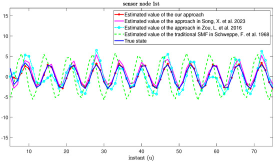
Figure 3. True state and its estimated values based on our approach and other approaches from [11,27,55].

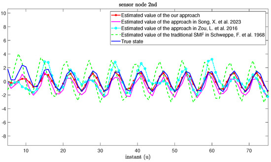
Figure 4. True state and its estimated values based on our approach and other approaches from [11,27,55].

Case 2. 

We consider the situation when cyber-attacks and MMs occur; the occurrences of attacks and MMs are shown below.

The occurrences of cyber-attacks and MMs are shown in Figure 5 and Figure 6, respectively.

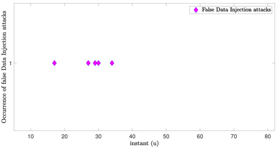
Figure 5. Occurrences of bias injection attacks.

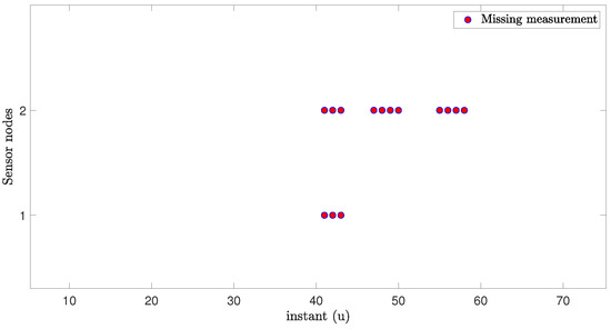
Figure 6. Occurrences of MMs on each sensor node.

Under the same parameters, the true state and the estimation values of the MNNs with MMs subject to cyber-attacks are shown below.

The real values $o_u^{\left(i\right)}$ and the estimation values ${\widehat{o}}_u^{\left(i\right)}(i=1,2)$ of the MNNs with MMs subject to cyber-attacks are shown in Figure 7 and Figure 8, respectively. From Figure 7 and Figure 8, we can see that the estimation framework we proposed in this paper can effectively estimate the true state of MNNs. When the system is threatened by cyber-attacks during transmission, the estimation error can increase accordingly. However, once the attack signal disappears, the estimation performance can recover immediately. In addition, when a sensor node exhibits an MM phenomenon, compared with the approaches based on the RR protocol in [27,55], our proposed algorithm can also reduce the influence of MMs on estimation performance.

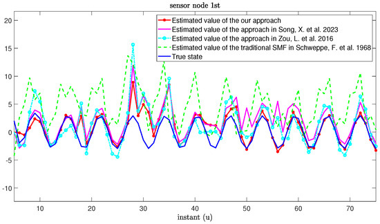
Figure 7. True state and its estimated values based on our approach and other approaches from [11,27,55].

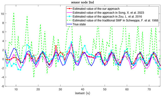
Figure 8. True state and its estimated values based on our approach and other approaches from [11,27,55].

The following figures show the sensor nodes selected to send the latest data at each sampling instant based on the WTOD protocol and RR protocol with MMs subject to cyber-attacks.

Figure 9 and Figure 10 show the situation of the sensor nodes sending data under the WTOD protocol and the RR protocol, respectively. From Figure 9 and Figure 10, we can see that only one sensor node sends data to the estimator at each sampling instant, which means that the use of these two protocols can save communication resources and reduce the communication burden when the network bandwidth is limited, in turn avoiding possible data collisions.

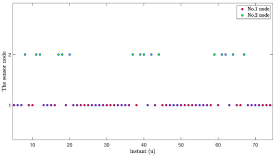
Figure 9. Selected nodes to transmit the latest data under the WTOD protocol.

Figure 10. Selected nodes to transmit the latest data under the RR protocol.

From Figure 5, Figure 6, Figure 7, Figure 8, Figure 9 and Figure 10, we can obtain that, when using the approaches based on the RR protocol in [27,55] to estimate the MNNs, the estimation performance can be greatly influenced once the sampling instants for the continuous occurrence of MMs exceeds the number of sensor nodes. In contrast, the state estimation results from the estimation framework proposed in this paper are more accurate, significantly less influenced by continuous occurrence of MMs. This is because, if we know that a certain sensor has a high occurrence probability of MMs, we can reduce the data transmission from this sensor to the estimator by changing the weight of the WTOD protocol, so as to reduce the sending of erroneous data to the estimator as much as possible.

Finally, to further confirm the practicability of the proposed estimation framework, we apply this framework to a real engineering problem.

Case 3. 

In this case, we consider a network-based test rig that consists of a plant (DC servo system) and a remote controller; the DC servo system is identified to be a third-order system, whose parameters are from [55]:

$$\left\{\begin{array}{c}{\overline{\tilde{o}}}_{u+1}=A{\overline{\tilde{o}}}_u+D{\overline{\tilde{o}}}_{u-{\tau }_1}+B{\overline{\tilde{W}}}_u\hfill \\ {\tilde{q}}_u={\alpha }_u(C{\overline{\tilde{o}}}_u+E{\overline{\tilde{V}}}_u)\hfill \\ {\overline{\tilde{o}}}_u={\overline{\Psi }}_u,u\in [-{\tau }_1,0]\hfill \end{array}\right.$$

$$\begin{array}{c}A=\left[\begin{array}{ccc}1.12& 0.213& -0.333\\ 1& 0& 0\\ 0& 1& 0\end{array}\right],B=\left[\begin{array}{c}0.8\\ 0\\ 0\end{array}\right],\hfill \\ D=\left[\begin{array}{ccc}-0.2193& 0.0219& 0.0844\\ 0.2177& -0.0032& -0.0662\\ 0.1298& -0.0087& -0.0381\end{array}\right],\hfill \\ C=\left[\begin{array}{ccc}1& 0& 0\\ 0& 1& 0\end{array}\right],E=\left[\begin{array}{c}0\\ 0.8\end{array}\right],\tilde{\omega }=\mathrm{diag}\{1.05,1\},\hfill \\ {\overline{\tilde{W}}}_u=0.5cos\left(0.2u\right),{\overline{\tilde{V}}}_u=0.5sin\left(0.2u\right),\hfill \\ R_{1,u}=R_{2,u}=0.25,P_u=\mathrm{diag}\{4,4,4,1,1\},\hfill \\ {\overline{\Psi }}_u=\left(222\right),{\tau }_1=3.\hfill \end{array}$$

The occurrence of MMs is referred to Case 2.

The real values $o_u^{\left(i\right)}$ and the estimation values ${\widehat{o}}_u^{\left(i\right)}(i=1,2,3)$ of the system with MMs and time delays are shown in Figure 11, Figure 12 andFigure 13, respectively.

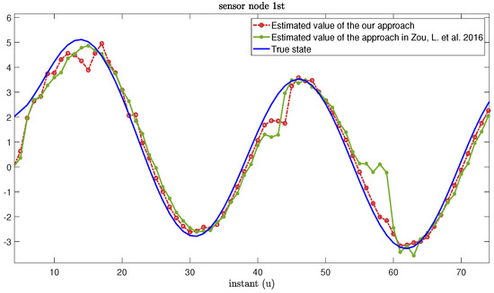
Figure 11. True state and its estimated values based on our approach and the approach from [55].

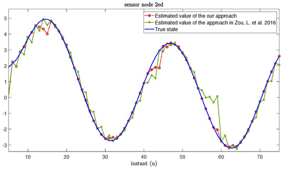
Figure 12. True state and its estimated values based on our approach and the approach from [55].

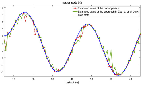
Figure 13. True state and its estimated values based on our approach and the approach from [55].

We compare our estimation framework with the approach proposed in [55]; we can see that our estimation framework can effectively reduce the influence of MMs and time delays on estimation performance. Therefore, Case 3 further verifies the effectiveness of the estimation framework proposed in this paper and its practicability in actual engineering scenarios.

5. Discussion

5.1. The Analysis of Experimental Results

In order to verify the estimation performance of the proposed estimation framework, we compare and calculate the computational load and mean square error (MSE) of the proposed approach and three common approaches for three cases.

The comparative estimation results of Case 1 are shown in Table 1 below.

Table 1. Estimation performance of Case 1.

Estimation Approach	Calculated Load (s)	Sum of the MSE
approach in [27]	24.213	2.010
approach in [55]	19.733	1.469
approach in [11]	7.462	8.134
our approach	21.452	0.297

According to Table 1, we can obtain that, in the absence of MMs and cyber-attacks, the sum of MSE of the approaches in [11,27,55] is higher than that of our approach by 85.22%, 79.78% and 96.34%, respectively, while the difference between their calculation load and our approach is within 3 seconds, except for [11]. Although the approach in [11] is fast, the accuracy is too low. Therefore, the comprehensive comparison shows that our approach is optimal when MNNs are not influenced by MMs and cyber-attacks.

The comparative estimation results of Case 2 are shown in Table 2 below.

Table 2. Estimation performance of Case 2.

Estimation Approach	Calculated Load (s)	Sum of the MSE	MSE during MMs
approach in [27]	31.462	2.081	61.156
approach in [55]	24.421	1.319	21.698
approach in [11]	8.421	8.127	75.927
our approach	26.597	0.251	13.251

According to Table 2, we can conclude that, in the presence of MNNs with MMs and cyber-attacks, the sum of MSE with the approaches in [11,27,55] are 87.93%, 79.78% and 96.91% higher than our approach, respectively. Furthermore, during MMs, their MSE values are 78.33%, 38.92% and 82.55% higher than our approach, respectively. The results show that, even when MNNs are influenced by MMs and cyber-attacks, our approach still has high estimation performance and can significantly reduce the influence of MMs on the estimation performance accuracy.

The comparative estimation results of Case 3 are shown in Table 3 below.

Table 3. Estimation performance of Case 3.

Estimation Approach	Calculated Load (s)	Sum of the MSE	MSE during MMs
approach in [55]	1.869	1.275	10.970
our approach	2.023	0.098	1.892

From the practical system case in Table 3, we can see that, compared with the approach in [55], the computational load of our approach is slightly lower, but the sum of MSE values during MM occurrence is 92.24% and 82.76% lower than the approach in [55]. This case also shows that the comprehensive estimation performance of our proposed estimation framework is better and practical.

5.2. Practicability of the Proposed Estimation Framework

In the “Simulation example” section, we verify the practicality of the proposed estimation framework through an engineering example. In fact, both cyber-attacks and MMs may occur in actual networked control systems, such as unmanned aerial vehicle group control systems and intelligent vehicle networking systems [63,64]. The estimation framework proposed in this paper is practical as long as the cyber-attacks obey the Bernoulli distribution.

6. Conclusions

This paper has investigated the non-fragile estimation problem based on set-membership filtering for a class of measurement-saturated MNNs with MMs and mixed time delays subject to stochastic cyber-attacks under the WTOD protocol. The occurrence of stochastic cyber-attacks follows a Bernoulli distribution. First, by utilizing the LMI technology, the estimation error has been ensured to still be limited within the specified ellipsoid despite the above sensor-related problems and network-induced phenomena. Simultaneously, through the set-membership filtering approach and mathematical induction, we have established the sufficient condition for the existence of the estimator, so that one can solve the LMI sequence to obtain the estimator gain. Moreover, by designing a non-fragile set-membership algorithm, the robustness of the estimation algorithm has been ensured under gain perturbation. Second, by solving the trace of the minimization matrix, the local optimal estimator gain has been obtained to achieve the optimal estimation performance at each sampling instant. Finally, numerical simulation examples have been presented to demonstrate the effectiveness of the proposed algorithm.

Although the estimation performance of the proposed estimation framework in this paper has been superior to other estimation frameworks proposed in the literature, when the MMs occur in a sensor node, if we do not know in advance which sensors have a higher probability of MMs, we cannot pre-set the weight values of the WTOD protocol, which greatly increases the probability of the estimator receiving missing data. Therefore, in future research, we should propose a dynamic communication strategy to detect the occurrence of MMs and adjust weights in real time to avoid the influence of MMs on estimation performance. In addition, for the occurrence of cyber-attacks, our estimation framework has still been passive to detect attacks and recover estimation performance. In some engineering scenarios, cyber-attacks influence the estimation performance, which may bring serious consequences to the whole system. Therefore, in the follow-up research, we hope to make improvements in the estimation framework to actively protect data from cyber-attacks.

References

- FAO. Memristive devices and systems. Proc. IEEE 1976, 64, 209–223. [Google Scholar] [CrossRef]
- Liu, H.; Wang, Z.; Shen, B.; Alsaadi, F. state estimation for discrete-time memristive recurrent neural networks with stochastic time-delays. Int. J. Gen. Syst. 2016, 45, 633–647. [Google Scholar] [CrossRef]
- Li, X.; Zhang, W.; Fang, J.; Li, H. Mixed H∞/L2 − L∞ State Estimation for Delayed Memristive Neural Networks with Markov Switching Parameters. Neurocomputing 2019, 340, 342–354. [Google Scholar] [CrossRef]
- Zhang, Y.; Zhou, L. State estimation for proportional delayed complex-valued memristive neural networks. Inf. Sci. 2024, 680, 121–150. [Google Scholar] [CrossRef]
- Ding, S.; Wang, Z.; Wang, J.; Zhang, H. H∞ state estimation for memristive neural networks with time-varying delays: The discrete-time case. Neural Netw. 2016, 84, 47–56. [Google Scholar] [CrossRef]
- Feng, L.; Zhao, L.; Ban, L. H∞ state estimation for discrete memristive neural networks with signal quantization and probabilistic time delay. Syst. Sci. Control Eng. 2021, 9, 764–774. [Google Scholar] [CrossRef]
- Xue, Z.; Zhang, Y.; Cheng, C.; Ma, G. Remaining useful life prediction of lithium-ion batteries with adaptive unscented kalman filter and optimized support vector regression. Neurocomputing 2020, 376, 95–102. [Google Scholar] [CrossRef]
- Liu, Y.; Wang, Z.; Liu, C.; Coombes, M.; Chen, W. Auxiliary Particle Filtering Over Sensor Networks Under Protocols of Amplify-and-Forward and Decode-and-Forward Relays. IEEE Trans. Signal Inf. Process. Over Netw. 2022, 8, 883–893. [Google Scholar] [CrossRef]
- Sheng, L.; Wang, Z.; Zou, L.; Alsaadi, F. Event-Based H∞ State Estimation for Time-Varying Stochastic Dynamical Networks With State- and Disturbance-Dependent Noises. IEEE Trans. Neural Netw. Learn. Syst. 2017, 28, 2382–2394. [Google Scholar] [CrossRef]
- Boada, B.L.; Boada, M.J.L.; Diaz, V. A robust observer based on energy-to-peak filtering in combination with neural networks for parameter varying systems and its application to vehicle roll angle estimation. Mechatronics 2018, 50, 196–204. [Google Scholar] [CrossRef]
- Schweppe, F. Recursive state estimation: Unknown but bounded errors and system inputs. IEEE Trans. Autom. Control 1968, 13, 22–28. [Google Scholar] [CrossRef]
- Zhao, Z.; Wang, Z.; Zou, L.; Liu, H.; Alsaadi, F. Zonotopic multi-sensor fusion estimation with mixed delays under try-once-discard protocol: A set-membership framework. Inf. Fusion 2023, 91, 681–693. [Google Scholar] [CrossRef]
- Gao, Y.; Ma, L.; Zhang, M.; Guo, J.; Bo, Y. Distributed Set-Membership Filtering for Nonlinear Time-Varying Systems With Dynamic Coding-Decoding Communication Protocol. IEEE Syst. J. 2022, 16, 2958–2967. [Google Scholar] [CrossRef]
- Wei, G.; Liu, S.; Song, Y.; Liu, Y. Probability-guaranteed set-membership filtering for systems with incomplete measurements. Automatica 2015, 60, 12–16. [Google Scholar] [CrossRef]
- Ding, D.; Wang, Z.; Han, Q. A Set-Membership Approach to Event-Triggered Filtering for General Nonlinear Systems Over Sensor Networks. IEEE Trans. Autom. Control 2020, 65, 1792–1799. [Google Scholar] [CrossRef]
- Zhao, Z.; Wang, Z.; Zou, L.; Chen, Y.; Sheng, W. Event-Triggered Set-Membership State Estimation for Complex Networks: A Zonotopes-Based Method. IEEE Trans. Netw. Sci. Eng. 2022, 9, 1175–1186. [Google Scholar] [CrossRef]
- Zhou, X.; Zhang, Y.; Chen, J.; Zheng, X. A quantized set-membership estimation-based heading control method of unmanned surface vessels under unknown-but-bounded wave-induced disturbances. Asian J. Control 2023, 25, 3105–3118. [Google Scholar] [CrossRef]
- Yang, H.; Zhang, Y.; Gu, W.; Yang, F.; Liu, Z. Set-membership filtering for automatic guided vehicles with unknown-but-bounded noises. Trans. Inst. Meas. Control 2022, 44, 716–725. [Google Scholar] [CrossRef]
- Yang, Y.; Hu, J.; Chen, D.; Wei, Y.; Du, J. Non-fragile Suboptimal Set-membership Estimation for Delayed Memristive Neural Networks with Quantization via Maximum-error-first Protocol. Int. J. Control Autom. Syst. 2020, 18, 1904–1914. [Google Scholar] [CrossRef]
- Hu, J.; Yang, Y.; Liu, H.; Chen, D.; Du, J. Non-fragile set-membership estimation for sensor-saturated memristive neural networks via weighted try-once-discard protocol. IET Control Theory Appl. 2020, 14, 1671–1680. [Google Scholar] [CrossRef]
- Liu, L.; Ma, L.; Zhang, J.; Bo, Y. Distributed non-fragile set-membership filtering for nonlinear systems under fading channels and bias injection attacks. Int. J. Syst. Sci. 2021, 52, 1192–1205. [Google Scholar] [CrossRef]
- Ma, L.; Wang, Z.; Lam, H.; Kyriakoulis, N. Distributed event-based set-Membership filtering for a Class of Nonlinear Systems with sensor saturations over sensor networks. IEEE Trans. Cybern. 2017, 47, 3772–3783. [Google Scholar] [CrossRef] [PubMed]
- Ma, L.; Wang, Z.; Lam, H. Event-triggered mean-square consensus control for time-varying stochastic multi-agent system with sensor saturations. IEEE Trans. Autom. Control 2017, 62, 3524–3531. [Google Scholar] [CrossRef]
- Ding, D.; Han, Q.; Ge, X. Distributed filtering of networked dynamic systems with non-gaussian noises over sensor networks: A survey. Kybernetika 2020, 56, 5–34. [Google Scholar] [CrossRef]
- Hu, J.; Li, J.; Kao, Y.; Chen, Y. Optimal distributed filtering for nonlinear saturated systems with random access protocol and missing measurements: The uncertain probabilities case. Appl. Math. Comput. 2022, 418, 235–246. [Google Scholar] [CrossRef]
- Yang, F.; Li, Y. Set-membership filtering for systems with sensor saturation. Automatica 2009, 45, 1896–1902. [Google Scholar] [CrossRef]
- Song, X.; Rong, L.; Li, B.; Wang, Z.; Li, J. Joint state and fault estimation for nonlinear systems with missing measurements and random component faults under Round-Robin Protocol. Int. J. Electr. Power Energy Syst. 2016, 154, 429–437. [Google Scholar] [CrossRef]
- Wei, G.; Wang, Z.; Shu, H. Robust filtering with stochastic nonlinearities and multiple missing measurements. Automatica 2009, 45, 836–841. [Google Scholar] [CrossRef]
- Hu, J.; Wang, Z.; Dong, H.; Gao, H. Recent Advances on Recursive Filtering and Sliding Mode Design for Networked Nonlinear Stochastic Systems: A Survey. Math. Probl. Eng. 2013, 32, 24–33. [Google Scholar] [CrossRef]
- Shen, B.; Wang, Z.; Wang, D.; Li, Q. State-Saturated Recursive Filter Design for Stochastic Time-Varying Nonlinear Complex Networks Under Deception Attacks. IEEE Trans. Neural Netw. Learn. Syst. 2020, 31, 3788–3800. [Google Scholar] [CrossRef]
- Liu, L.; Ma, L.; Wang, Y.; Zhang, J.; Bo, Y. Distributed set-membership filtering for time-varying systems under constrained measurements and replay attacks. J. Frankl.-Inst.-Eng. Appl. Math. 2020, 357, 4983–5003. [Google Scholar] [CrossRef]
- Geng, H.; Wang, Z.; Hu, J.; Alsaadi, F.; Cheng, Y. Outlier-resistant sequential filtering fusion for cyber-physical systems with quantized measurements under denial-of-service attacks. Inf. Sci. 2023, 628, 488–503. [Google Scholar] [CrossRef]
- Hu, L.; Wang, Z.; Han, Q.; Liu, X. State estimation under false data injection attacks: Security analysis and system protection. Automatica 2018, 87, 176–183. [Google Scholar] [CrossRef]
- Zhao, D.; Wang, Z.; Wei, G.; Han, Q. A dynamic event-triggered approach to observer-based PID security control subject to deception attacks. Automatica 2020, 120, 891–900. [Google Scholar] [CrossRef]
- Xu, W.; Wang, Z.; Hu, L.; J, J. State estimation under joint false data injection attacks: Dealing with constraints and insecurity. IEEE Trans. Autom. Control 2022, 67, 6745–6753. [Google Scholar] [CrossRef]
- Li, T.; Wang, Z.; Zou, L.; Chen, B.; Yu, L. A dynamic encryption-decryption scheme for replay attack detection in cyber-physical systems. Automatica 2023, 151, 34–47. [Google Scholar] [CrossRef]
- Wang, X.; Ding, D.; Ge, X.; Han, Q. Neural-network-based control for discrete-time nonlinear systems with denial-of-service attack: The adaptive event-triggered case. IEEE/CAA J. Autom. Sin. 2022, 32, 2760–2779. [Google Scholar] [CrossRef]
- Xiao, S.; Ge, X.; Han, Q.; Zhang, Y. Secure Distributed Adaptive Platooning Control of Automated Vehicles Over Vehicular Ad-Hoc Networks Under Denial-of-Service Attacks. IEEE Trans. Cybern. 2022, 52, 12003–12015. [Google Scholar] [CrossRef]
- Ding, D.; Liu, H.; Dong, H.; Liu, H. Resilient Filtering of Nonlinear Complex Dynamical Networks Under Randomly Occurring Faults and Hybrid Cyber-Attacks. IEEE Trans. Netw. Sci. Eng. 2022, 9, 2341–2352. [Google Scholar] [CrossRef]
- Li, M.; Liang, J. State estimation for 2-D uncertain systems with redundant channels and deception attacks: A set-membership method. Appl. Math. Comput. 2023, 457, 3184–3194. [Google Scholar] [CrossRef]
- Zhao, Z.; Wang, Z.; Zou, L.; Guo, J. Set-membership filtering for time-varying complex networks with uniform quantisations over randomly delayed redundant channels. Int. J. Syst. Sci. 2020, 51, 3364–3377. [Google Scholar] [CrossRef]
- Li, J.; Wei, G.; Ding, D.; Li, Y. Set-membership filtering for discrete time-varying nonlinear systems with censored measurements under Round-Robin protocol. Neurocomputing 2018, 281, 20–26. [Google Scholar] [CrossRef]
- Li, X.; Han, F.; Hou, N.; Dong, H.; Liu, H. Set-membership filtering for piecewise linear systems with censored measurements under Round-Robin protocol. Int. J. Syst. Sci. 2020, 51, 1578–1588. [Google Scholar] [CrossRef]
- Rana, M.; Li, L.; Su, S. Cyber Attack Protection and Control of Microgrids. IEEE-CAA J. Autom. Sin. 2018, 5, 602–609. [Google Scholar] [CrossRef]
- Qu, B.; Wang, Z.; Shen, B.; Dong, H. Secure Particle Filtering With Paillier Encryption-Decryption Scheme: Application to Multi-machine Power Grids. IEEE Trans. Smart Grid 2023, 15, 863–873. [Google Scholar] [CrossRef]
- Luan, X.; Shi, Y.; Liu, F. Unscented Kalman Filtering For Greenhouse Climate Control Systems With Missing Measurement. Int. J. Innov. Comput. Inf. Control. 2012, 8, 2173–2180. [Google Scholar]
- Befekadu, G.K.; Gupta, V.; Antsaklis, P.J. Risk-Sensitive Control Under Markov Modulated Denial-of-Service (DoS) Attack Strategies. IEEE Trans. Autom. Control 2015, 60, 3299–3304. [Google Scholar] [CrossRef]
- Yi, X.; Yu, H.; Wang, P.; Liu, S.; Ma, L. Encoding–decoding-based secure filtering for neural networks under mixed attacks. Neurocomputing 2020, 508, 71–78. [Google Scholar] [CrossRef]
- Zou, L.; Wang, Z.; Hu, J.; Gao, H. On H∞ Finite-Horizon Filtering Under Stochastic Protocol: Dealing With High-Rate Communication Networks. IEEE Trans. Autom. Control 2017, 62, 4884–4890. [Google Scholar] [CrossRef]
- Zhu, K.; Hu, J.; Liu, Y.; Alotaibi, N.; Alsaadi, F. On L2 − L∞ output-feedback control scheduled by stochastic communication protocol for two-dimensional switched systems. Int. J. Syst. Sci. 2021, 52, 2961–2976. [Google Scholar] [CrossRef]
- Li, J.; Wang, Z.; Dong, H.; Fei, W. Delay-distribution-dependent state estimation for neural networks under stochastic communication protocol with uncertain transition probabilities. Neural Netw. 2020, 130, 143–151. [Google Scholar] [CrossRef] [PubMed]
- Li, B.; Wang, Z.; Han, Q.; Liu, H. Distributed Quasiconsensus Control for Stochastic Multiagent Systems Under Round-Robin Protocol and Uniform Quantization. IEEE Trans. Cybern. 2022, 52, 6721–6732. [Google Scholar] [CrossRef] [PubMed]
- Li, M.; Liang, J.; Wang, F. Robust set-membership filtering for two-dimensional systems with sensor saturation under the Round-Robin protocol. Int. J. Syst. Sci. 2022, 53, 2773–2785. [Google Scholar] [CrossRef]
- Li, X.; Dong, H.; Wang, Z.; Han, F. Set-membership filtering for state-saturated systems with mixed time-delays under weighted try-once-discard protocol. Automatica 2018, 74, 341–348. [Google Scholar] [CrossRef]
- Zou, L.; Wang, Z.; Gao, H. Set-membership filtering for time-varying systems with mixed time-delays under Round-Robin and Weighted Try-Once-Discard protocols. Automatica 2016, 74, 341–348. [Google Scholar] [CrossRef]
- Shen, Y.; Wang, Z.; Shen, B.; Dong, H. Outlier-resistant recursive filtering for multisensor multirate networked systems under weighted try-once-discard protocol. IEEE Trans. Cybern. 2021, 51, 4897–4908. [Google Scholar] [CrossRef]
- Wang, F.; Liang, J.; Lam, J.; Yang, J.; Zhao, C. Robust Filtering for 2-D Systems With Uncertain-Variance Noises and Weighted Try-Once-Discard Protocols. IEEE Trans. Syst. Man-Cybern.-Syst. 2023, 53, 2914–2924. [Google Scholar] [CrossRef]
- Zou, L.; Wang, Z.; Hu, J.; Liu, Y.; Liu, X. Communication-protocol-based analysis and synthesis of networked systems: Progress, prospects and challenges. Int. J. Syst. Sci. 2021, 52, 3013–3034. [Google Scholar] [CrossRef]
- Yang, H.; Yan, H.; Zhou, J.; Zhang, Y.; Chang, Y. Neural-Network-Based Set-Membership Filtering Under WTOD Protocols via a Novel Event-Triggered Compensation Mechanism. IEEE Trans. Syst. Man, Cybern. Syst. 2024, 54, 2954–2964. [Google Scholar] [CrossRef]
- Li, X.; Gong, R.; Zhu, L. Interval Observer Design for Nonlinear Interconnected Systems via Ellipsoid Approach. Int. J. Control Autom. Syst. 2024, 22, 807–815. [Google Scholar] [CrossRef]
- Boyd, S.; Ghaoui, L.; Feron, E.; Balakrishnan, V. Linear Matrix Inequalities in System and Control Theory; SIAM: Philadelphia, PA, USA, 1994; Volume 15. [Google Scholar]
- Khalil, H. Nonlinear Systems; Prentice Hall: Hoboken, NJ, USA, 2002. [Google Scholar]
- Ge, X.; Han, Q.; Wu, Q.; Zhang, X. Resilient and Safe Platooning Control of Connected Automated Vehicles Against Intermittent Denial-of-Service Attacks. IEEE-CAA J. Autom. Sin. 2023, 10, 1234–1251. [Google Scholar] [CrossRef]
- Zhang, J.; Ren, Z.; Deng, C.; Wen, B. Adaptive fuzzy global sliding mode control for trajectory tracking of quadrotor UAVs. Nonlinear Dyn. 2019, 97, 609–627. [Google Scholar] [CrossRef]
Disclaimer/Publisher’s Note: The statements, opinions and data contained in all publications are solely those of the individual author(s) and contributor(s) and not of MDPI and/or the editor(s). MDPI and/or the editor(s) disclaim responsibility for any injury to people or property resulting from any ideas, methods, instructions or products referred to in the content. |
© 2024 by the authors. Licensee MDPI, Basel, Switzerland. This article is an open access article distributed under the terms and conditions of the Creative Commons Attribution (CC BY) license (https://creativecommons.org/licenses/by/4.0/).