
Interruption Cost Estimation for Value-Based Reliability Investment in Emerging Smart Grid Resources


Abstract
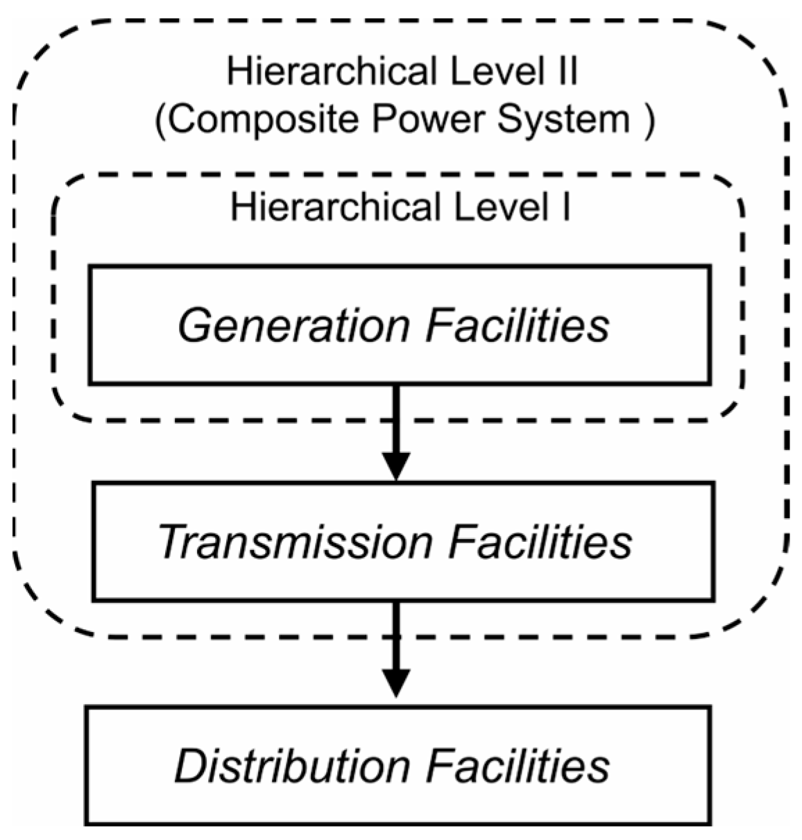
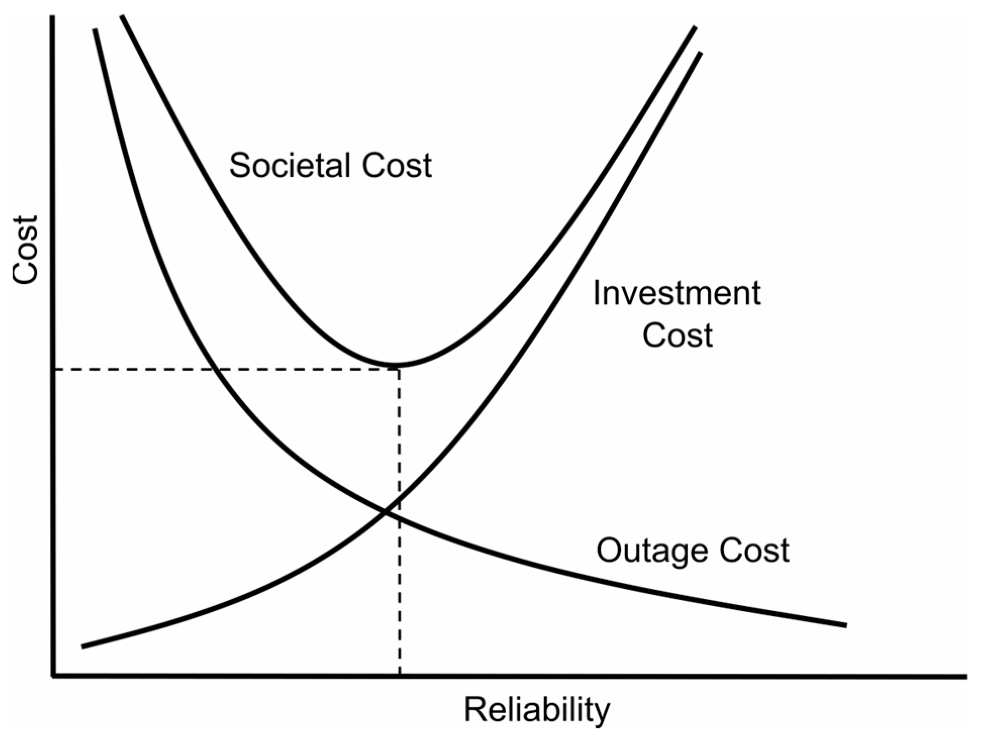
1. Introduction
2. Estimation of Interruption Costs Arising from Transmission System Originated Failures
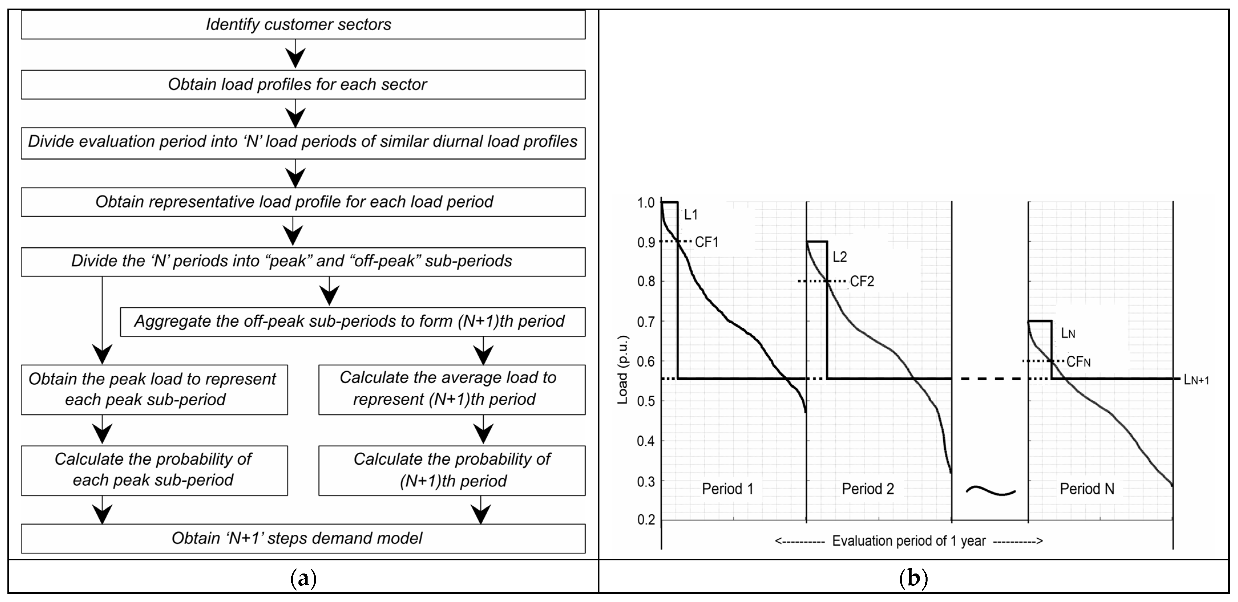
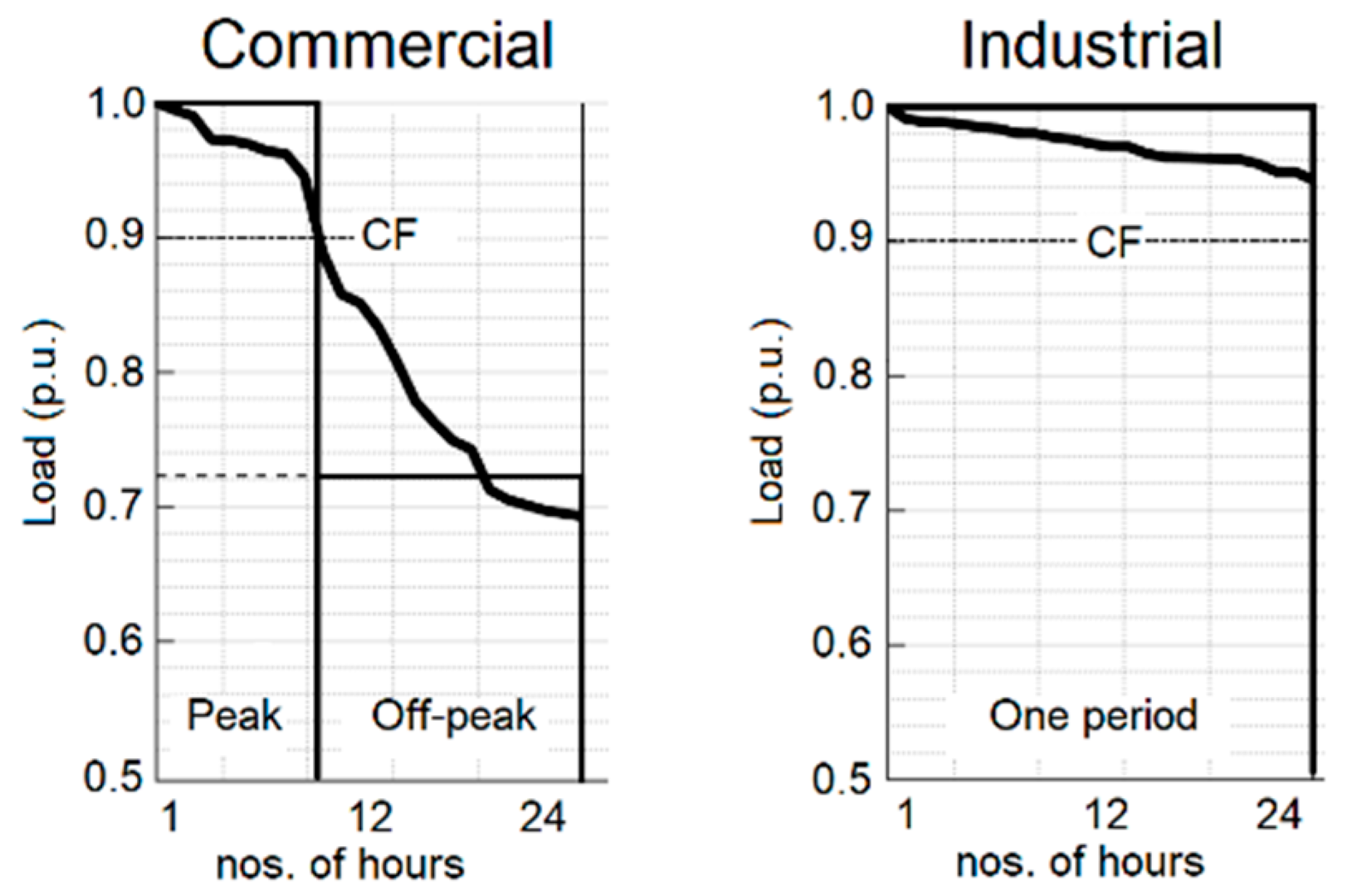
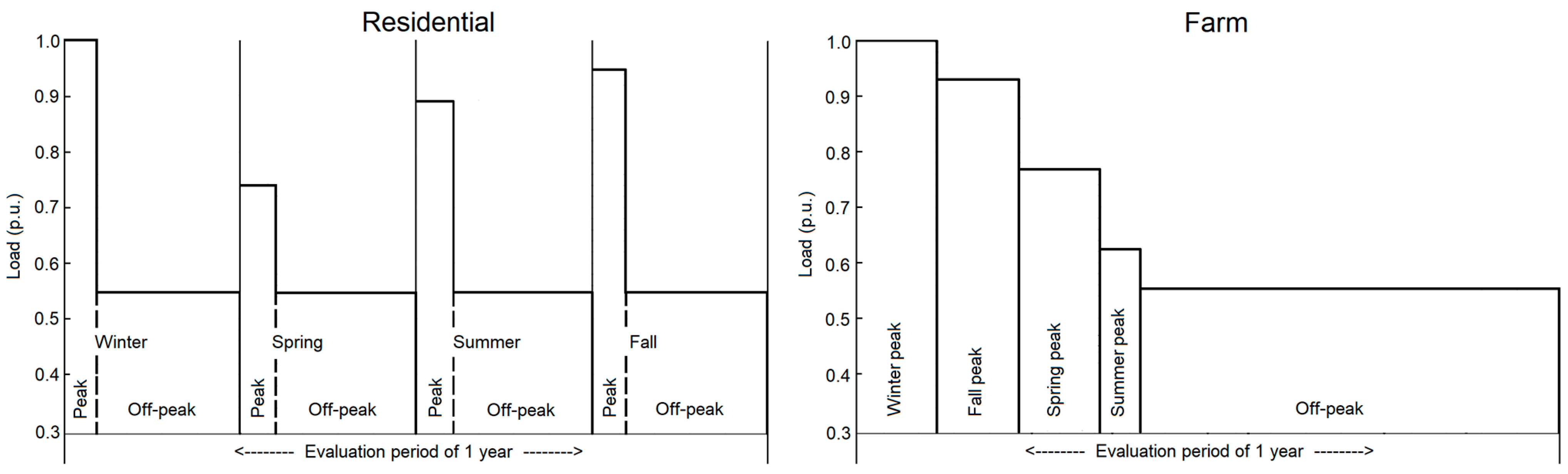
2.1. Sector Periodic Demand Model
2.2. Integrated Interruption Cost Model
3. Illustration of the Methodology
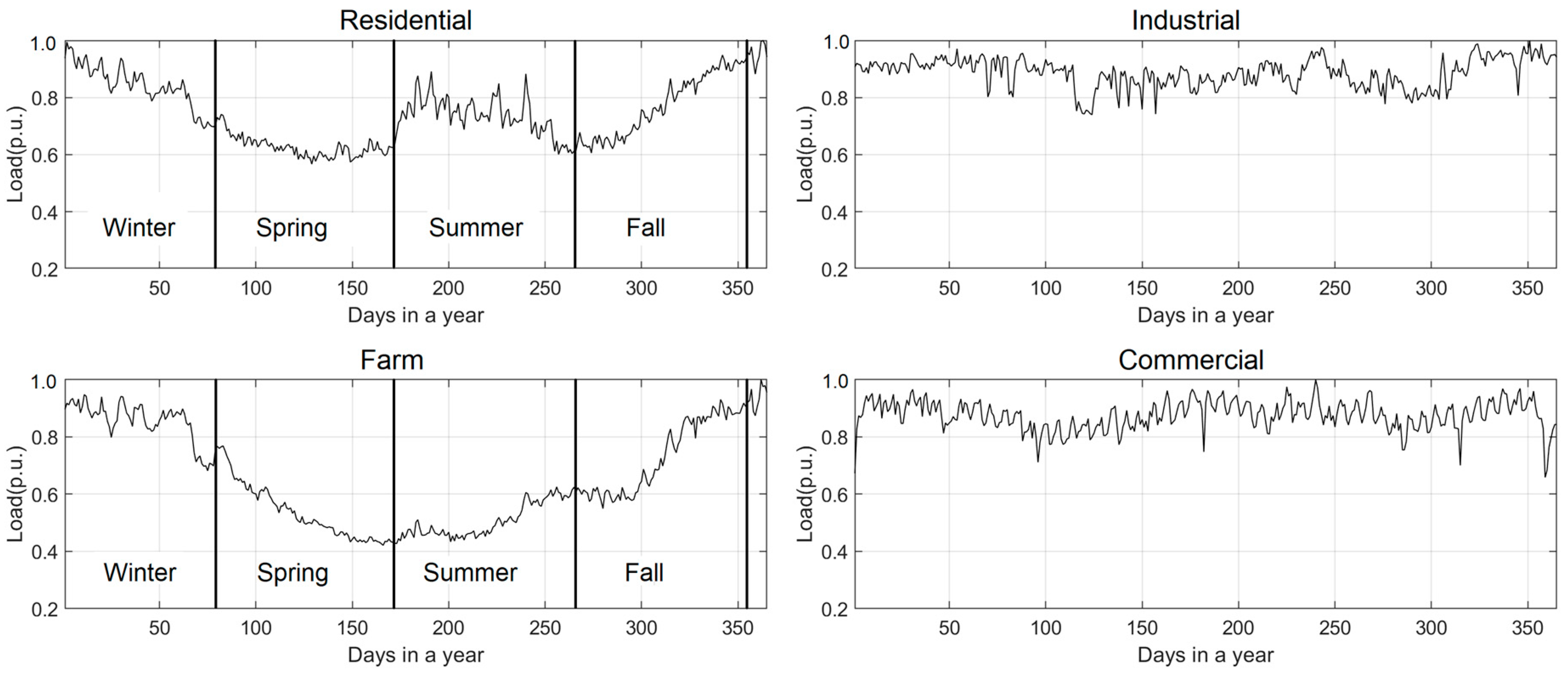
3.1. Obtaining the SPD Model
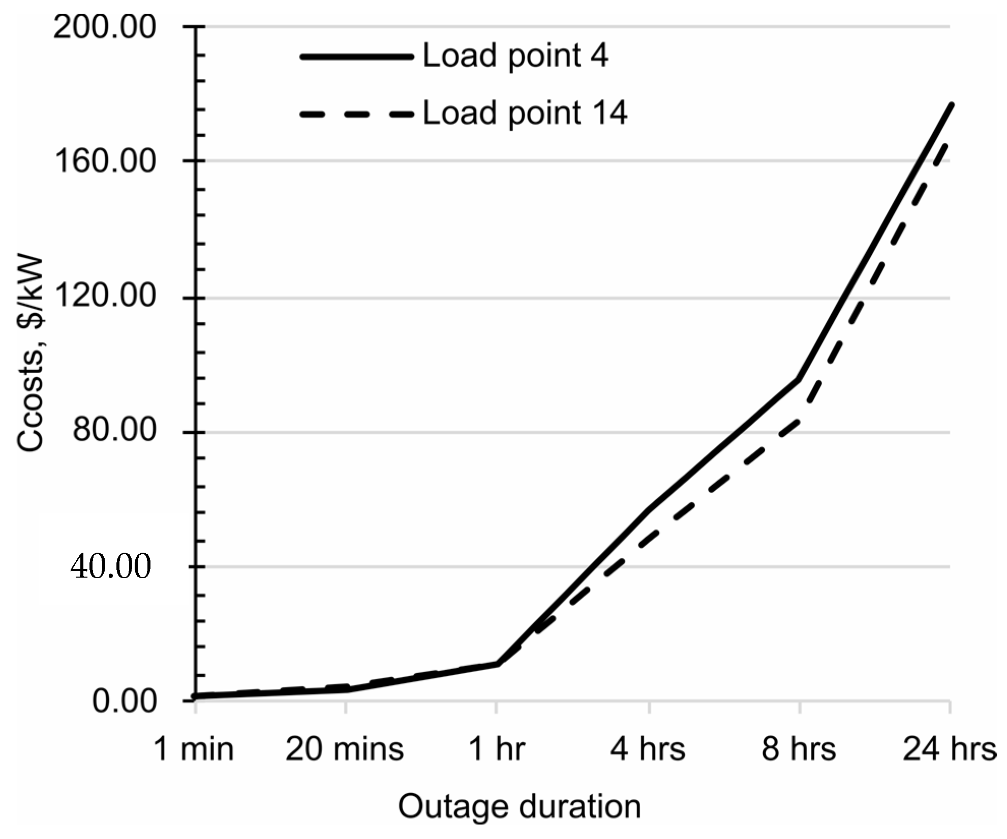
3.2. Obtaining the Integrated Interruption Cost Model
4. Conclusions
Author Contributions
Funding
Institutional Review Board Statement
Informed Consent Statement
Data Availability Statement
Conflicts of Interest
References
- Billinton, R.; Allan, R.N. Reliability Evaluation of Power Systems; Springer: Boston, MA, USA, 1996; ISBN 978-1-4899-1862-8. [Google Scholar]
- Billinton, R. Evaluation of Reliability Worth in an Electric Power System. Reliab. Eng. Syst. Saf. 1994, 46, 15–23. [Google Scholar] [CrossRef]
- Billinton, R.; Oteng-Adjei, J. Cost/Benefit Approach to Establish Optimum Adequacy Level for Generating System Planning. IEE Proc. C Gener. Transm. Distrib. 1988, 135, 81. [Google Scholar] [CrossRef]
- Billinton, R.; Goel, L. A Procedure for Estimating the Overall System Worth Associated with Generating Unit Refurbishment. Can. J. Electr. Comput. Eng. 1990, 15, 140–148. [Google Scholar] [CrossRef]
- Billinton, R.; Adzanu, S. Adequacy and Reliability Cost/Worth Implications of Nonutility Generation. IEE Proc. Gener. Transm. Distrib. 1996, 143, 115. [Google Scholar] [CrossRef]
- Sarkar, A. Reliability Evaluation of a Generation-Resource Plan Using Customer-Outage Costs in India. Energy 1996, 21, 795–803. [Google Scholar] [CrossRef]
- Billinton, R.; Pandey, M. Generating Capacity Planning Criteria Determination for Developing Countries-Case Study of Nepal. IEE Proc. Gener. Transm. Distrib. 1999, 146, 491. [Google Scholar] [CrossRef]
- Prada, J.F.; Ilic, M.D. Pricing Reliability: A Probabilistic Approach. In Proceedings of the Large Engineering Systems Conference on Power Engineering, Halifax, NS, Canada, 20–22 June 1999. [Google Scholar]
- Gen, B. Reliability and Cost/Worth Evaluation of Generating Systems Utilizing Wind and Solar Energy. Ph.D. Thesis, University of Saskatchewan, Saskatoon, SK, Canada, 2005. [Google Scholar]
- Bagen, B.; Billinton, R. Reliability Cost/Worth Associated with Wind Energy and Energy Storage Utilization in Electric Power Systems. In Proceedings of the 10th International Conference on Probabilistic Methods Applied to Power Systems, Rincon, PR, USA, 25–29 May 2008. [Google Scholar]
- Limbu, T.R.; Saha, T.K.; McDonald, J.D.F. Value-Based Allocation and Settlement of Reserves in Electricity Markets. IET Gener. Transm. Distrib. 2011, 5, 489. [Google Scholar] [CrossRef]
- Oteng-Adjei, J.; Malori, A.-M.I.; Anto, E.K. Generation System Adequacy Assessment Using Analytical Technique. In Proceedings of the 2020 IEEE PES/IAS PowerAfrica, Nairobi, Kenya, 25–28 August 2020; pp. 1–5. [Google Scholar]
- Billinton, R.; Tollefson, G.; Wacker, G. Assessment of Electric Service Reliability Worth. Int. J. Electr. Power Energy Syst. 1993, 15, 95–100. [Google Scholar] [CrossRef]
- Wacker, G.; Wojczynski, E.; Billinton, R. Interruption Cost Methodology and Results—A Canadian Residential Survey. IEEE Trans. Power Appar. Syst. 1983, PAS-102, 3385–3392. [Google Scholar] [CrossRef]
- Wojczynski, E.; Billinton, R.; Wacker, G. Interruption Cost Methodology and Results—A Canadian Commercial and Small Industry Survey. IEEE Trans. Power Appar. Syst. 1984, PAS-103, 437–444. [Google Scholar] [CrossRef]
- Wacker, G.; Billinton, R. Farm Losses Resulting from Electric Service Interruptions—A Canadian Survey. IEEE Trans. Power Syst. 1989, 4, 472–478. [Google Scholar] [CrossRef]
- Tollefson, G.; Billinton, R.; Wacker, G.; Chan, E.; Aweya, J. A Canadian Customer Survey to Assess Power System Reliability Worth. IEEE Trans. Power Syst. 1994, 9, 443–450. [Google Scholar] [CrossRef]
- Lawton, L.; Sullivan, M.; Van Liere, K.; Katz, A.; Eto, J. A Framework and Review of Customer Outage Costs: Integration and Analysis of Electric Utility Outage Cost Surveys; Lawrence Berkeley National Laboratory: Berkeley, CA, USA, 2003. [Google Scholar]
- Sullivan, M.J.; Mercurio, M.; Schellenberg, J. Estimated Value of Service Reliability for Electric Utility Customers in the United States; Lawrence Berkeley National Laboratory: Berkeley, CA, USA, 2009; p. LBNL-2132E, 963320. [Google Scholar]
- Sanghvi, A.P. Economic Costs of Electricity Supply Interruptions: US and Foreign Experience. Energy Econ. 1982, 4, 180–198. [Google Scholar] [CrossRef]
- Wacker, G.; Tollefson, G. Electric Power System Customer Interruption Cost Assessment. Reliab. Eng. Syst. Saf. 1994, 46, 75–81. [Google Scholar] [CrossRef]
- Outage Cost Estimation Guidebook. Available online: https://www.epri.com/research/products/TR-106082 (accessed on 11 December 2022).
- TPL-001-5; Transmission System Planning Performance Requirements. North American Electric Reliability Corporation (NERC): Washington, DC, USA.
- Papic, M.; Logan, D. Bibliography on Composite System Reliability Assessment 2000–2020. In Proceedings of the 2022 17th International Conference on Probabilistic Methods Applied to Power Systems (PMAPS), Manchester, UK, 12–15 June 2022; pp. 1–8. [Google Scholar]
- Billion-Dollar Weather and Climate Disasters | National Centers for Environmental Information (NCEI). Available online: https://www.ncei.noaa.gov/access/billions/ (accessed on 20 May 2023).
- Bhattarai, S.; Sapkota, A.; Karki, R. Analyzing Investment Strategies for Power System Resilience. In Proceedings of the 2022 IEEE Power & Energy Society General Meeting (PESGM), Denver, CO, USA, 17–21 July 2022; pp. 1–5. [Google Scholar]
- Gasser, P.; Lustenberger, P.; Cinelli, M.; Kim, W.; Spada, M.; Burgherr, P.; Hirschberg, S.; Stojadinovic, B.; Sun, T.Y. A Review on Resilience Assessment of Energy Systems. Sustain. Resilient Infrastruct. 2021, 6, 273–299. [Google Scholar] [CrossRef]
- Lin, Y. A Review of Key Strategies in Realizing Power System Resilience. Glob. Energy Interconnect. 2018, 1, 9. [Google Scholar]
- Wenyuan, L.; Billinton, R. A Minimum Cost Assessment Method for Composite Generation and Transmission System Expansion Planning. IEEE Trans. Power Syst. 1993, 8, 628–635. [Google Scholar] [CrossRef]
- Siddiqi, S.N.; Baughman, M.L. Value-Based Transmission Planning and the Effects of Network Models. IEEE Trans. Power Syst. 1995, 10, 1835–1842. [Google Scholar] [CrossRef]
- Choi, J.; Mount, T.D.; Thomas, R.J.; Billinton, R. Probabilistic Reliability Criterion for Planning Transmission System Expansions. IEE Proc. Gener. Transm. Distrib. 2006, 153, 719. [Google Scholar] [CrossRef]
- Choi, J.S.; Tran, T.T.; Kang, S.R.; Jeon, D.H.; Lee, C.H.; Billinton, R. A Study on the Optimal Reliability Criteria Decision for a Transmission System Expansion Planning. In Proceedings of the IEEE Power Engineering Society General Meeting, 2004, Denver, CO, USA, 6–10 June 2004; Volume 1, pp. 607–613. [Google Scholar]
- Chowdhury, A.A.; Koval, D.O. Reliability Cost-Benefit Evaluation of Transmission Capital Projects. In Proceedings of the 2006 IEEE Power Engineering Society General Meeting, Montreal, QC, Canada, 18–22 June 2006; pp. 607–613. [Google Scholar]
- Billinton, R.; Wangdee, W. Reliability-Based Transmission Reinforcement Planning Associated With Large-Scale Wind Farms. IEEE Trans. Power Syst. 2007, 22, 34–41. [Google Scholar] [CrossRef]
- Oliveira, G.C.; Binato, S.; Pereira, M.V.F. Value-Based Transmission Expansion Planning of Hydrothermal Systems Under Uncertainty. IEEE Trans. Power Syst. 2007, 22, 1429–1435. [Google Scholar] [CrossRef]
- Leite Da Silva, A.M.; Rezende, L.S.; Da Fonseca Manso, L.A.; De Resende, L.C. Reliability Worth Applied to Transmission Expansion Planning Based on Ant Colony System. Int. J. Electr. Power Energy Syst. 2010, 32, 1077–1084. [Google Scholar] [CrossRef]
- Sullivan, M.; Schellenberg, J.; Blundell, M. Updated Value of Service Reliability Estimates for Electric Utility Customers in the United States; Lawrence Berkeley National Laboratory: Berkeley, CA, USA, 2015; p. LBNL-6941E, 1172643. [Google Scholar]
- Dalton, J.G.; Garrison, D.L.; Fallon, C.M. Value-Based Reliability Transmission Planning. IEEE Trans. Power Syst. 1996, 11, 1400–1408. [Google Scholar] [CrossRef]
- Brandenburg, L.; Clarkson, G.; Leo, J.; Asbury, J.; Brandon-Brown, F.; Derderian, H.; Mueller, R.; Swaroop, R. Load Research Manual. Volume 1. Load Research Procedures; Argonne National Lab. (ANL): Argonne, IL, USA; National Economic Research Associates: New York, NY, USA, 1980. [Google Scholar]
- Puckett, C.; Williamson, C.; Godin, C.; Gifford, W.; Farland, J.; Laing, T.; Hong, T. Utility Load Research: The Future of Load Research Is Now. IEEE Power Energy Mag. 2020, 18, 61–70. [Google Scholar] [CrossRef]
- Billinton, R.; Zhang, W. Cost Related Reliability Evaluation of Bulk Power Systems. Int. J. Electr. Power Energy Syst. 2001, 23, 99–112. [Google Scholar] [CrossRef]
- Wacker, G.; Billinton, R. Customer Cost of Electric Service Interruptions. Proc. IEEE 1989, 77, 919–930. [Google Scholar] [CrossRef]
- Karki, N.R.; Karki, R. Outage Cost Assessment for Value Based Reliability Investment in System Generating Capacity; Technical Report Prepared for Saskatchewan Power Corporation; University of Saskatchewan: Saskatoon, SK, Canada, 2018. [Google Scholar]
- Inflation Calculator. Available online: https://www.bankofcanada.ca/rates/related/inflation-calculator/ (accessed on 19 August 2023).


| Period | Load (p.u. of Sector Peak) | Probability |
|---|---|---|
| Residential | ||
| Winter peak | 1.0000 | 0.009247 |
| Spring peak | 0.7410 | 0.003767 |
| Summer peak | 0.8913 | 0.003196 |
| Fall peak | 0.9489 | 0.010300 |
| Off-peak | 0.5470 | 0.973500 |
| Farm | ||
| Winter peak | 1.0000 | 0.011758 |
| Spring peak | 0.7685 | 0.006279 |
| Summer peak | 0.6254 | 0.006507 |
| Fall peak | 0.9305 | 0.019064 |
| Off-peak | 0.5538 | 0.956393 |
| Commercial | ||
| Peak | 1.0000 | 0.068493 |
| Off-peak | 0.7227 | 0.931507 |
| Industrial | ||
| One period | 1.0000 | 1.000000 |
| Sector | 1 min | 20 min | 1 h | 4 h | 8 h | 24 h |
|---|---|---|---|---|---|---|
| Residential | 0.00 | 0.54 | 4.06 | 45.52 | 92.78 | 352.07 |
| Farm | 1.83 | 8.06 | 13.98 | 24.32 | 26.83 | 52.37 |
| Commercial | 29.69 | 87.81 | 237.21 | 1194.95 | 1920.18 | 2312.68 |
| Industrial | 252,912.00 | 417,959.00 | 822,855.00 | 2,719,105.00 | 5,239,916.00 | 15,431,217.00 |
| Sector | Residential | Farm | Commercial | Industrial |
|---|---|---|---|---|
| Sector peak (kW) | 2.0461 | 2.7000 | 8.1000 | 99,780.0000 |
| Sector | 1 min | 20 min | 1 h | 4 h | 8 h | 24 h |
|---|---|---|---|---|---|---|
| One period | 2.53 | 4.19 | 8.25 | 27.25 | 52.51 | 154.65 |
| Actions | No Action | Provide Minimal Lighting | Provide Full Lighting and LED TVs | Lighting, TVs and Small Appliances (Fan) | Full Household Load |
|---|---|---|---|---|---|
| Cost (CAD/h.) | 0.0 | 1.0 | 6.0 | 12.0 | 25.0 |
| Undesirability | None | Low | Moderate Low | Moderate High | High | Extremely Undesirable |
|---|---|---|---|---|---|---|
| Scale | 1 | 2 | 3 | 4 | 5 | 6 |
| Likert Scale (4 h) | 1 | 2 | 3 | 4 | 5 | 6 | Cost, CAD/int |
|---|---|---|---|---|---|---|---|
| Winter peak (weekly) | 4 | 3 | 5 | 14 | 35 | 162 | 82.28 |
| Winter peak (monthly) | 11 | 22 | 39 | 41 | 53 | 57 | 45.97 |
| Winter off-peak (weekly) | 6 | 12 | 15 | 31 | 45 | 113 | 65.82 |
| Spring peak (weekly) | 14 | 12 | 35 | 50 | 51 | 61 | 47.70 |
| Summer peak (weekly) | 10 | 30 | 39 | 51 | 37 | 56 | 43.30 |
| Fall peak (weekly) | 10 | 13 | 24 | 58 | 55 | 62 | 48.92 |
| Period | (2023, CAD/int) |
|---|---|
| Winter peak | 45.97 |
| Spring peak | 26.71 |
| Summer peak | 24.25 |
| Fall peak | 27.40 |
| Off-peak | 24.87 |
| Period | 1 min | 20 min | 1 h | 4 h | 8 h | 24 h |
|---|---|---|---|---|---|---|
| Winter peak | 0.00 | 0.55 | 4.09 | 45.97 | 93.69 | 355.58 |
| Spring peak | 0.00 | 0.32 | 2.38 | 26.71 | 54.43 | 206.60 |
| Summer peak | 0.00 | 0.29 | 2.16 | 24.25 | 49.42 | 187.57 |
| Fall peak | 0.00 | 0.33 | 2.44 | 27.40 | 55.84 | 211.94 |
| Off-peak | 0.00 | 0.30 | 2.21 | 24.87 | 50.69 | 192.37 |
| Period | 1 min | 20 min | 1 h | 4 h | 8 h | 24 h |
|---|---|---|---|---|---|---|
| Farm | ||||||
| Winter peak | 1.83 | 8.06 | 13.98 | 24.32 | 26.83 | 52.37 |
| Spring peak | 1.06 | 4.68 | 8.12 | 14.13 | 15.59 | 30.43 |
| Summer peak | 0.97 | 4.26 | 7.38 | 12.84 | 14.17 | 27.65 |
| Fall peak | 1.09 | 4.80 | 8.33 | 14.49 | 15.99 | 31.20 |
| Off-peak | 0.99 | 4.36 | 7.56 | 13.16 | 14.52 | 28.34 |
| Commercial | ||||||
| Peak | 29.69 | 87.81 | 237.21 | 1194.95 | 1920.18 | 2312.68 |
| Off-peak | 16.03 | 47.52 | 128.32 | 646.47 | 1038.81 | 1251.18 |
| Period | 1 min | 20 min | 1 h | 4 h | 8 h | 24 h |
|---|---|---|---|---|---|---|
| Residential | ||||||
| Winter peak | 0.00 | 0.27 | 2.00 | 22.47 | 45.79 | 173.78 |
| Spring peak | 0.00 | 0.21 | 1.57 | 17.62 | 35.90 | 136.26 |
| Summer peak | 0.00 | 0.16 | 1.18 | 13.30 | 27.10 | 102.85 |
| Fall peak | 0.00 | 0.17 | 1.26 | 14.11 | 28.76 | 109.16 |
| Off-peak | 0.00 | 0.27 | 1.97 | 22.22 | 45.29 | 171.88 |
| Farm | ||||||
| Winter peak | 0.68 | 2.99 | 5.18 | 9.01 | 9.94 | 19.40 |
| Spring peak | 0.51 | 2.26 | 3.91 | 6.81 | 7.51 | 14.67 |
| Summer peak | 0.57 | 2.52 | 4.37 | 7.60 | 8.39 | 16.37 |
| Fall peak | 0.43 | 1.91 | 3.32 | 5.77 | 6.36 | 12.42 |
| Off-peak | 0.66 | 2.92 | 5.06 | 8.80 | 9.71 | 18.95 |
| Commercial | ||||||
| Peak | 3.67 | 10.84 | 29.29 | 147.52 | 237.06 | 285.52 |
| Off-peak | 3.00 | 8.89 | 24.00 | 120.93 | 194.32 | 234.04 |
| Sector | 1 min | 20 min | 1 h | 4 h | 8 h | 24 h |
|---|---|---|---|---|---|---|
| Residential | 0.00 | 0.27 | 1.96 | 22.09 | 45.03 | 170.90 |
| Farm | 0.65 | 2.89 | 5.02 | 8.72 | 9.63 | 18.79 |
| Commercial | 3.05 | 9.02 | 24.36 | 122.75 | 197.25 | 237.57 |
| Industrial | 2.53 | 4.19 | 8.25 | 27.25 | 52.51 | 154.65 |
| Sector | Peak Demand % | Energy Consumption % | ||
|---|---|---|---|---|
| Load Point 4 | Load Point 14 | Load Point 4 | Load Point 14 | |
| Residential | 40% | 19% | 45% | 14% |
| Farm | 15% | 10% | 10% | 6% |
| Commercial | 30% | 25% | 35% | 24% |
| Industrial | 15% | 46% | 10% | 56% |
Disclaimer/Publisher’s Note: The statements, opinions and data contained in all publications are solely those of the individual author(s) and contributor(s) and not of MDPI and/or the editor(s). MDPI and/or the editor(s) disclaim responsibility for any injury to people or property resulting from any ideas, methods, instructions or products referred to in the content. |
© 2024 by the authors. Licensee MDPI, Basel, Switzerland. This article is an open access article distributed under the terms and conditions of the Creative Commons Attribution (CC BY) license (https://creativecommons.org/licenses/by/4.0/).
Share and Cite
Bhattarai, S.; Karki, R. Interruption Cost Estimation for Value-Based Reliability Investment in Emerging Smart Grid Resources. Appl. Sci. 2024, 14, 8651. https://doi.org/10.3390/app14198651
Bhattarai S, Karki R. Interruption Cost Estimation for Value-Based Reliability Investment in Emerging Smart Grid Resources. Applied Sciences. 2024; 14(19):8651. https://doi.org/10.3390/app14198651
Chicago/Turabian StyleBhattarai, Shandesh, and Rajesh Karki. 2024. "Interruption Cost Estimation for Value-Based Reliability Investment in Emerging Smart Grid Resources" Applied Sciences 14, no. 19: 8651. https://doi.org/10.3390/app14198651
APA StyleBhattarai, S., & Karki, R. (2024). Interruption Cost Estimation for Value-Based Reliability Investment in Emerging Smart Grid Resources. Applied Sciences, 14(19), 8651. https://doi.org/10.3390/app14198651