Online Trajectory Replanning for Avoiding Moving Obstacles Using Fusion Prediction and Gradient-Based Optimization

Abstract

In this study, we introduce a novel method for an online trajectory replanning approach for fixed-wing Unmanned Aerial Vehicles (UAVs). Our method integrates moving obstacle predictions within a gradient-based optimization framework. The trajectory is represented by uniformly discretized waypoints, which serve as the optimization variables within the cost function. This cost function incorporates multiple objectives, including obstacle avoidance, kinematic and dynamic feasibility, similarity to the reference trajectory, and trajectory smoothness. To enhance prediction accuracy, we combine physics-based and pattern-based methods for predicting obstacle movements. These predicted movements are then integrated into the online trajectory replanning framework, significantly enhancing the system’s safety. Our approach provides a robust solution for navigating dynamic environments, ensuring both optimal and secure UAV operation.

1. Introduction

Unmanned Aerial Vehicles (UAVs) are extensively applied across various fields, including monitoring missions [1,2], surveillance [3,4,5], and transportation [6,7,8], demonstrating significant value and potential. UAVs typically follow a global reference trajectory to complete their missions. Nevertheless, to guarantee secure and autonomous navigation in unstructured environments, trajectory replanning becomes a critical area of research. This is essential to adapt to dynamic and unpredictable conditions, enabling UAVs to avoid obstacles and respond effectively to changes in their surroundings.

The challenge of trajectory replanning has been a central focus in extensive research efforts. In [9], a structured search space based on state lattice motion primitives was developed for quadrotor micro-UAVs to navigate cluttered and partially known environments. Similarly, ref. [10] introduced two families of motion primitives for fixed-wing UAVs, facilitating online path planning through forests while ensuring the capability for emergency turnaround maneuvers. Furthermore, ref. [11] utilized a motion primitive library to select collision-free maneuvers, enabling high-speed navigation through forests using only onboard vision and planning. Despite their utility, these motion primitive-based methods require discretization of both the workspace and the state space, with their performance being highly dependent on the number of generated motion primitives.

Another strategy involves generating numerous path candidates cost-effectively and selecting the optimal one based on an objective function. In [12], a sampling-based partial motion planning method along a reference path was introduced. Moreover, ref. [13] introduced a method that iteratively generates trajectory samples targeting low-cost areas within the sampling space. However, their reliance on randomly sampled trajectories to identify collision-free paths may be problematic in densely cluttered environments.

Drawing inspiration from CHOMP [14,15], gradient-based optimization has become a widely used approach for replanning. In [16], a local replanning system was constructed by optimizing polynomial trajectories. Similarly, ref. [17] integrated a sampling-based topological path searching approach with path-guided B-splines trajectory optimization for real-time UAV replanning. Optimization-based trajectory replanning has achieved significant success, leading to numerous subsequent methods built upon this foundation (e.g., [18,19,20]). However, these approaches typically involve many parameters (e.g., control points for B-splines and polynomial coefficients) that require careful tuning. More importantly, these methods do not anticipate the motion of surrounding moving obstacles, which is a critical prerequisite for safe and efficient motion planning [21].

In this work, we present an online trajectory replanning approach specifically designed for fixed-wing UAVs, which incorporates predictions for moving obstacles into a gradient-based optimization framework. Our method represents the trajectory using uniformly discretized waypoints, serving as the basis for defining the optimization cost function. This function incorporates multiple objectives, including obstacle avoidance, kinematic and dynamic constraints, similarity to the reference trajectory, and trajectory smoothness. Additionally, moving obstacles are predicted by combining physics-based methods with pattern-based methods, allowing for the predicted obstacle movements to be integrated into the local trajectory replanning framework. This integration enhances the safety of the system.

2. Method

In this work, we consider for the fixed-wing UAV with low-level control the following nonholonomic model in 2D

$$\left\{\begin{array}{c}\dot{x}=v\cos \phi \hfill \\ \dot{y}=v\sin \phi ,\hfill & v_{min}\le v\le v_{max}\hfill \\ \dot{\phi }=\omega ,\hfill & \left|\omega \right|\le {\omega }_{max}\hfill \end{array}\right.$$

(1)

where $(x,y)\in {\mathbb{R}}^2$ represents the UAV’s position, and $\phi \in (-\pi ,\pi ]$ denotes its heading angle. v represents the forward velocity, and $\omega$ is the turn rate. The constraints $v_{min}$ and $v_{max}$ define the minimum and maximum airspeeds, respectively, while ${\omega }_{max}$ limits the turn rate.

Low-level control systems like the Piccolo autopilot [22] and the MicroPilot autopilot [23] are capable of decoupling the longitudinal and lateral dynamics of small fixed-wing UAVs. This allows us to focus solely on lateral trajectory planning, ensuring compliance with dynamic constraints. The altitude dynamics are omitted, as our primary interest lies in the lateral plane.

Before delving into the topic of trajectory replanning, it is essential to discuss the generation of a global reference trajectory. In known and structured environments, various methods can be employed to create a global reference trajectory from the starting point to the destination. For instance, one could utilize a topologically feasible straight-line path generated by $A^{*}$ [24,25] or $RRT$ [26,27] and then refine it into a dynamically feasible trajectory through trajectory optimization [28]. Alternatively, a global trajectory can be predefined by experts. These predefined trajectories are generally well constructed but are not equipped to handle unexpected situations, particularly the presence of dynamic obstacles.

Given a known global trajectory, we can utilize established trajectory tracking algorithms [29,30] during real-time operations. However, during a fixed-wing UAV mission, moving obstacles may be encountered, such as other non-cooperative aircraft or mobile targets. These obstacles, though not intentionally interfering with our flight path, are unpredictable and their motion trajectories may not be known or easily obtainable in real time. Therefore, our algorithm aims to monitor and predict the motion trajectories of these dynamic obstacles in real time.

By predicting the movement of these obstacles, we can assess the safety of the global reference trajectory. If a segment of the local trajectory is predicted to collide with a moving target, we can select two points from the global reference trajectory as the start and end points for local trajectory replanning. Subsequently, we perform online trajectory replanning to avoid potential collisions.

In this work, we represent the waypoints of a trajectory using $\xi ={[x,y,\phi ]}^T$. Suppose the fixed starting and ending waypoints of the replanned trajectory are ${\xi }_0$ and ${\xi }_f$, respectively. We employ a uniform discretization method, sampling the replanned trajectory function between ${\xi }_0$ and ${\xi }_f$ at equal time steps of length $\delta t$. Consequently, our waypoint trajectory representation can be denoted as $\mathcal{T}\in {\mathcal{R}}^{3n}$:

$$\mathcal{T}=\left[\begin{array}{c}{\xi }_1\hfill \\ {\xi }_2\hfill \\ \dots \hfill \\ {\xi }_n\hfill \end{array}\right]$$

(2)

where each ${\xi }_i$ represents a waypoint in the trajectory.

Given this trajectory representation, our objective is to find a local replanned trajectory $\mathcal{T}$ that can avoid moving obstacles based on the proposed motion prediction algorithm. This replanned trajectory should closely follow the global reference trajectory while maintaining smoothness and dynamic feasibility. In other words, it must satisfy the airspeed and turn rate constraints of the fixed-wing UAV.

2.1. Obstacle Prediction Using Fusion Prediction

To predict obstacle motion, we first present physics-based techniques using the constant velocity model (CVM), followed by pattern-based methods with kernelized movement primitive (KMP). Finally, we describe how these two approaches are combined to improve prediction accuracy.

2.1.1. Physics-Based Prediction: CVM

In this work, we employ the constant velocity model (CVM) as our physics-based approach due to its strong performance and simplicity [31].

The CVM assumes that an obstacle maintains a constant velocity over a short prediction horizon, simplifying the prediction process while providing reasonably accurate forecasts for the near future. Suppose at time step i, we detect a moving target with position coordinates $(x_i^o,y_i^o)$, airspeed $v_i^o$, and heading angle ${\phi }_i^o$. Using these variables, the state of the moving obstacle can be denoted as ${\xi }_i^o={[x_i^o,y_i^o,{\phi }_i^o]}^T$. The state of the moving obstacle at the next time step $i+1$ can be expressed as follows:

$${\xi }_{i+1}^o={\xi }_i^o+v_i^o\left[\begin{array}{c}\cos {\phi }_i^o\hfill \\ \sin {\phi }_i^o\hfill \\ 0\hfill \end{array}\right]\Delta t+w_i,w_i\sim \mathcal{N}(0,Q_i)$$

(3)

where $w_i$ are stochastic processes representing the uncertainty in the model, characterized as Gaussian, zero-mean, white noise, and independent random variables.

2.1.2. Pattern-Based Prediction: KMP

Despite the simplicity and effectiveness of the CVM, pattern-based prediction holds a distinct advantage in its ability to learn from data. Unlike physics-based approaches that rely on predefined, parameterized functions to model motion dynamics, pattern-based methods adhere to a Sense–Learn–Predict framework. This framework enables the model to derive motion dynamics directly from data, thereby potentially enhancing prediction accuracy in complex environments.

In our research, we utilize kernelized movement primitive (KMP) [32,33,34] as our pattern-based model.

Consider K historical trajectories of length J, denoted as ${\{{\{{\xi }_{j,k}^o,{\xi }_{j+1,k}^o\}}_{j=1}^J\}}_{k=1}^K$. Initially, we employ the Gaussian Mixture Model (GMM) [35] and Gaussian Mixture Regression (GMR) [36] to obtain a probabilistic reference trajectory ${\{{\xi }_n^o,{\hat{\overrightarrow{\mu }}}_n,{\widehat{\overrightarrow{\mathsf{\Sigma }}}}_n\}}_{n=1}^N$ (for further details, please refer to [32]). Next, KMPs are utilized to capture and generalize the probabilistic reference trajectory. Specifically, the prediction function is expressed as follows:

$$f^{pred}({\xi }_n^o)=\mathsf{\Theta }{({\xi }_n^o)}^T\overrightarrow{w}$$

(4)

where $\mathsf{\Theta }({\xi }_n^o)$ is a known matrix composed of basis functions, and $\overrightarrow{w}$ is the weight vector that follows the distribution

$$\overrightarrow{w}\sim \mathcal{N}({\overrightarrow{\mu }}_{\overrightarrow{w}},{\overrightarrow{\mathsf{\Sigma }}}_{\overrightarrow{w}})$$

(5)

where the mean ${\overrightarrow{\mu }}_{\overrightarrow{w}}$ and the covariance ${\overrightarrow{\mathsf{\Sigma }}}_{\overrightarrow{w}}$ are unknown. The optimal solutions for ${\overrightarrow{\mu }}_{\overrightarrow{w}}^{*}$ and ${\overrightarrow{\mathsf{\Sigma }}}_{\overrightarrow{w}}^{*}$ can be derived using the dual transformation of the kernel ridge regression (KRR) [37], as detailed in [32,37,38]:

$$\begin{array}{c}{\overrightarrow{\mu }}_{\overrightarrow{w}}^{*}=\overrightarrow{\mathsf{\Phi }}{({\overrightarrow{\mathsf{\Phi }}}^T\overrightarrow{\mathsf{\Phi }}+{\lambda }_{\mu }\overrightarrow{\mathsf{\Sigma }})}^{-1}\overrightarrow{\mu }\hfill \\ {\overrightarrow{\mathsf{\Sigma }}}_{\overrightarrow{w}}^{*}=N{(\overrightarrow{\mathsf{\Phi }}{\overrightarrow{\mathsf{\Sigma }}}^{-1}{\overrightarrow{\mathsf{\Phi }}}^T+{\lambda }_{\mathsf{\Sigma }}\overrightarrow{I})}^{-1}\hfill \end{array}$$

(6)

where

$$\begin{array}{cc}\hfill \overrightarrow{\mathsf{\Phi }}& =[\mathsf{\Theta }({\xi }_1^o)\mathsf{\Theta }({\xi }_2^o)\cdots \mathsf{\Theta }({\xi }_N^o)]\hfill \\ \hfill \overrightarrow{\mathsf{\Sigma }}& =blockdiag({\widehat{\overrightarrow{\mathsf{\Sigma }}}}_1,{\widehat{\overrightarrow{\mathsf{\Sigma }}}}_2,\dots ,{\widehat{\overrightarrow{\mathsf{\Sigma }}}}_N),\hfill \\ \hfill \overrightarrow{\mu }& ={[{\hat{\overrightarrow{\mu }}}_1^T{\hat{\overrightarrow{\mu }}}_2^T\cdots {\hat{\overrightarrow{\mu }}}_N^T]}^T.\hfill \end{array}$$

(7)

and ${\lambda }_{\mu },{\lambda }_{\mathsf{\Sigma }}>0$ are regularization parameters to prevent overfitting [39].

The kernel function $k({\xi }_i^o,{\xi }_j^o)$ allows us to avoid explicitly defining the basis function. Consequently, the kernel matrix can be computed as

$$\overrightarrow{k}({\xi }_i^o,{\xi }_j^o)=\mathsf{\Theta }{({\xi }_i^o)}^T\mathsf{\Theta }({\xi }_J^o)=k({\xi }_i^o,{\xi }_j^o)\overrightarrow{I}$$

(8)

Therefore, for a query ${\xi }_{*}^o$, the expected value of the prediction $f^{pred}({\xi }_{*}^o)$ is given by

$$\mathbf{E}(f^{pred}({\xi }_{*}^o))={\overrightarrow{k}}^{*}{(\overrightarrow{K}+{\lambda }_{\mu }\overrightarrow{\mathsf{\Sigma }})}^{-1}\overrightarrow{\mu }$$

(9)

with

$$\overrightarrow{K}=\left[\begin{array}{cccc}\overrightarrow{k}({\xi }_1^o,{\xi }_1^o)& \overrightarrow{k}({\xi }_1^o,{\xi }_2^o)& \cdots & \overrightarrow{k}({\xi }_1^o,{\xi }_N^o)\\ \overrightarrow{k}({\xi }_2^o,{\xi }_1^o)& \overrightarrow{k}({\xi }_2^o,{\xi }_2^o)& \cdots & \overrightarrow{k}({\xi }_2^o,{\xi }_N^o)\\ ⋮& ⋮& \ddots & ⋮\\ \overrightarrow{k}({\xi }_N^o,{\xi }_1^o)& \overrightarrow{k}({\xi }_N^o,{\xi }_2^o)& \cdots & \overrightarrow{k}({\xi }_N^o,{\xi }_N^o)\end{array}\right]$$

(10)

and

$${\overrightarrow{k}}^{*}=\left[\begin{array}{cccc}\overrightarrow{k}({\xi }_{*}^o,{\xi }_1^o)& \overrightarrow{k}({\xi }_{*}^o,{\xi }_2^o)& \cdots & \overrightarrow{k}({\xi }_{*}^o,{\xi }_N^o)\end{array}\right]$$

(11)

The covariance of $f^{pred}({\xi }_{*}^o)$ is

$$\mathbf{D}(f^{pred}({\xi }_{*}^o))={\displaystyle \frac{N}{{\lambda }_{\mathsf{\Sigma }}}}({\overrightarrow{k}}^{**}-{\overrightarrow{k}}^{*}{(\overrightarrow{K}+{\lambda }_{\mathsf{\Sigma }}\overrightarrow{\mathsf{\Sigma }})}^{-1}{\overrightarrow{k}}^{{*}^T})$$

(12)

with

$${\overrightarrow{k}}^{**}=\overrightarrow{k}({\xi }_{*}^o,{\xi }_{*}^o)$$

(13)

By leveraging KMP, we can intelligently predict the future positions of moving obstacles. This non-parametric approach is suitable for online learning in complex environments.

2.1.3. Integration of Prediction Methods

We consider integrating the physics-based prediction CVM and pattern-based prediction KMP to provide a comprehensive obstacle prediction system.

Suppose at the i-th time step, the mean and covariance of the moving target are ${\hat{\xi }}_i^o$ and ${\hat{P}}_i^o$, respectively. The challenge is to compute the mean and covariance at the next time step $i+1$ using both the CVM and KMP.

The physics-based prediction CVM updates the mean and covariance as follows:

$$\begin{array}{c}{\hat{\xi }}_i^{o,\mathrm{CVM}}={\hat{\xi }}_i^o+{\overrightarrow{u}}_n\hfill \\ {\hat{P}}_i^{o,\mathrm{CVM}}={\hat{P}}_i^o+Q_i\hfill \end{array}$$

(14)

where ${\overrightarrow{u}}_n$ and $Q_i$ are obtained according to (3).

The pattern-based prediction KMP updates the mean and covariance as follows:

$$\begin{array}{c}{\hat{\xi }}_i^{o,\mathrm{KMP}}=\mathbf{E}(f^{pred}({\hat{\xi }}_i^o))\hfill \\ {\hat{P}}_i^{o,\mathrm{KMP}}=\mathbf{D}(f^{pred}({\hat{\xi }}_i^o))\hfill \end{array}$$

(15)

To integrate the predictions from both methods, we use a weighted fusion approach. Let ${\overrightarrow{W}}_i$ be the weighting factor for the CVM and $\overrightarrow{I}-{\overrightarrow{W}}_i$ be the weighting factor for the KMP. The fused mean ${\hat{\xi }}_{i+1}^o$ and covariance ${\hat{P}}_{i+1}^o$ at time step $i+1$ are computed as follows:

$$\begin{array}{c}{\hat{\xi }}_{i+1}^o={\overrightarrow{W}}_i{\hat{\xi }}_i^{o,\mathrm{CVM}}+(\overrightarrow{I}-{\overrightarrow{W}}_i){\hat{\xi }}_i^{o,\mathrm{KMP}}\hfill \\ {\hat{P}}_{i+1}^o={\overrightarrow{W}}_i{\hat{P}}_i^{o,\mathrm{CVM}}{\overrightarrow{W}}_i^T+(\overrightarrow{I}-{\overrightarrow{W}}_i){\hat{P}}_i^{o,\mathrm{KMP}}{(\overrightarrow{I}-{\overrightarrow{W}}_i)}^T\hfill \end{array}$$

(16)

We seek ${\overrightarrow{W}}_i$ that minimizes ${\hat{P}}_{i+1}^o$ by setting ${\displaystyle \frac{\partial {\hat{P}}_{i+1}^o}{\partial {\overrightarrow{W}}_i}}$ to $\overrightarrow{0}$, i.e.,

$${\displaystyle \frac{\partial {\hat{P}}_{i+1}^o}{\partial {\overrightarrow{W}}_i}}={\hat{P}}_i^{o,\mathrm{CVM}}{\overrightarrow{W}}_i+{\hat{P}}_i^{o,\mathrm{KMP}}(\overrightarrow{I}-{\overrightarrow{W}}_i)=\overrightarrow{0}$$

(17)

Solving this equation, we derive the optimal ${\overrightarrow{W}}_i^{*}$ as

$${\overrightarrow{W}}_i^{*}={\hat{P}}_i^{o,\mathrm{KMP}}{({\hat{P}}_i^{o,\mathrm{CVM}}+{\hat{P}}_i^{o,\mathrm{KMP}})}^{-1}$$

(18)

Using ${\overrightarrow{W}}_i^{*}$, we can compute the optimal fused mean ${\hat{\xi }}_{i+1}$ and covariance ${\hat{P}}_{i+1}^o$:

$$\begin{array}{c}{\hat{\xi }}_{i+1}^o={\overrightarrow{W}}_i^{*}{\hat{\xi }}_i^{o,\mathrm{CVM}}+(\overrightarrow{I}-{\overrightarrow{W}}_i^{*}){\hat{\xi }}_i^{o,\mathrm{KMP}}\hfill \\ {\hat{P}}_{i+1}^o={\overrightarrow{W}}_i^{*}{\hat{P}}_i^{o,\mathrm{CVM}}{\overrightarrow{W}}_i^T+(\overrightarrow{I}-{\overrightarrow{W}}_i^{*}){\hat{P}}_i^{o,\mathrm{KMP}}{(\overrightarrow{I}-{\overrightarrow{W}}_i^{*})}^T\hfill \end{array}$$

(19)

This integration approach leverages the strengths of both the CVM and KMP to provide a robust prediction system for moving obstacles. It should be noted that to predict a sequence of state transitions, successive one-step predictions are performed to construct an extended long-term trajectory.

2.2. Trajectory Replanning Using Gradient-Based Optimization

Local trajectory replanning can be modeled as an unconstrained optimization problem. The cost function consists of five terms and is computed as follows:

$$\mathbb{J}(\mathcal{T})={\lambda }_c{\mathbb{J}}_c(\mathcal{T})+{\lambda }_d{\mathbb{J}}_c(\mathcal{T})+{\lambda }_k{\mathbb{J}}_k(\mathcal{T})+{\lambda }_r{\mathbb{J}}_r(\mathcal{T})+{\lambda }_s{\mathbb{J}}_s(\mathcal{T})$$

(20)

where ${\mathbb{J}}_c$ is a collision cost based on the prediction of moving obstacles; ${\mathbb{J}}_d$ is the dynamic feasibility cost, which penalizes an infeasible airspeed and turn rate; ${\mathbb{J}}_k$ is the kinematic constraint cost, which penalizes deviations from the nonholonomic motion constraints of the UAV; ${\mathbb{J}}_r$ penalizes the distance between the global reference trajectory and the replanned trajectory; and ${\mathbb{J}}_s$ represents the trajectory smoothness cost. Each term is weighted by a corresponding coefficient to balance their contributions to the overall cost function.

2.2.1. Collision Cost Function

The collision cost function aims to guide the trajectory away from moving obstacles based on their predicted motion.

At the i-th time step, the state of a moving obstacle is predicted as ${\hat{\xi }}_i^o$, and the replanned waypoint is denoted as ${\xi }_i$. The distance between the replanned trajectory and the moving obstacle $d_i$ can be computed:

$$d_i=\sqrt{{({\xi }_i-{\hat{\xi }}_i^o-{\Delta }_{\phi })}^T({\xi }_i-{\hat{\xi }}_i^o-{\Delta }_{\phi })}$$

(21)

where ${\Delta }_{\phi }$ is used to ensure that the difference in the third component $\phi$ is zero, focusing our calculation on the distance between the 2D positions.

Our goal is to maintain a distance between the UAV and obstacles that exceeds $d_{safe}$. Thus, the collision cost function can be designed as follows:

$${\mathbb{J}}_c=\sum _{i=1}^{n}exp(-{\alpha }_c(d_i-d_{safe}))$$

(22)

where ${\alpha }_c$ is a positive scaling factor that determines the sensitivity of the cost to the distance. The exponential function is used to penalize distances that are close to or less than the safe threshold $d_{safe}$, with the cost rapidly increasing as the distance decreases. This formulation ensures that trajectories maintaining a safe distance from obstacles are favored, effectively minimizing the risk of collision.

2.2.2. Dynamic Feasibility Cost Function

The dynamic feasibility cost function ensures the trajectory adheres to physical constraints, such as a feasible airspeed and turn rate.

Let ${\overrightarrow{S}}_v=\left[\begin{array}{cc}{\overrightarrow{I}}_2& {\overrightarrow{0}}_{2\times 1}\end{array}\right]$ and ${\overrightarrow{S}}_{\phi }=\left[\begin{array}{ccc}0& 0& 1\end{array}\right]$ be the selection matrices for the airspeed and turn rate, respectively. Then, we can design the dynamic feasibility cost function for the airspeed as

$${\mathbb{J}}_{d,v}=\sum _{i=0}^{n}exp({\alpha }_v(\parallel {\overrightarrow{S}}_v{\displaystyle \frac{{\xi }_{i+1}-{\xi }_i}{\Delta t}}\parallel -v_{max}))+exp(-{\alpha }_v(\parallel {\overrightarrow{S}}_v{\displaystyle \frac{{\xi }_{i+1}-{\xi }_i}{\Delta t}}\parallel -v_{min}))$$

(23)

Similarly, we can design the dynamic feasibility cost function for the turn rate as follows:

$${\mathbb{J}}_{d,\omega }=\sum _{i=0}^{n}exp({\alpha }_{\omega }(\parallel {\overrightarrow{S}}_{\phi }{\displaystyle \frac{{\xi }_{i+1}-{\xi }_i}{\Delta t}}{\parallel }^2-{\omega }_{max}^2))$$

(24)

where ${\alpha }_v,{\alpha }_{\omega }$ are positive scaling factors. Thus, the dynamic feasibility cost function is represented as follows:

$${\mathbb{J}}_d={\lambda }_v{\mathbb{J}}_{d,v}+{\lambda }_{\omega }{\mathbb{J}}_{d,\omega }$$

(25)

where ${\lambda }_v,{\lambda }_{\omega }$ are the weighting coefficients.

2.2.3. Kinematic Constraint Cost Function

The kinematic constraint cost function ensures that the replanned trajectory adheres to the nonholonomic motion constraints specific to fixed-wing UAVs.

It is crucial to recognize that the movement of fixed-wing UAVs is intrinsically coupled in the xy-coordinate plane. Consequently, when planning the trajectory, it is crucial to verify that each waypoint satisfies the kinematic requirements of the UAV. Specifically, the subsequent waypoint should align with the UAV’s current heading direction. Failure to do so could result in a trajectory that is incompatible with the UAV’s motion capabilities. This consideration is a key innovation in addressing the unique challenges posed by fixed-wing UAVs.

Therefore, we design the kinematic constraint cost function as follows:

$${\mathbb{J}}_k=\sum _{i=0}^n{c}_i^2$$

(26)

with

$$c_i=\left\{\begin{array}{c}tan({\xi }_i\left[3\right])-{\displaystyle \frac{{\xi }_{i+1}\left[2\right]-{\xi }_i\left[2\right]}{{\xi }_{i+1}\left[1\right]-{\xi }_i\left[1\right]}}if{\xi }_{i+1}\left[1\right]\ne {\xi }_i\left[1\right],\hfill \\ tan({\xi }_i\left[3\right])-sign({\xi }_{i+1}\left[2\right]-{\xi }_i\left[2\right]){\displaystyle \frac{\pi }{2}}if{\xi }_{i+1}\left[1\right]={\xi }_i\left[1\right].\hfill \end{array}\right.$$

(27)

Here, ${\xi }_i\left[1\right],{\xi }_i\left[2\right],{\xi }_i\left[3\right]$ represent the first, second, and third elements of ${\xi }_i$, respectively. The term $c_i$ quantifies the deviation between the UAV’s heading direction and the direction of the trajectory segment connecting waypoints ${\xi }_i$ and ${\xi }_{i+1}$. Minimizing this cost function ensures that the trajectory maintains compatibility with the UAV’s kinematic constraints, thereby enhancing overall navigation performance.

By carefully designing and minimizing this kinematic constraint cost function, we address the core challenge of maintaining a feasible and efficient trajectory for fixed-wing UAVs in complex environments.

2.2.4. Reference Trajectory Cost Function

The reference trajectory cost function is designed to align the replanned trajectory with the pre-optimized reference trajectory. This cost term is defined as follows:

$${\mathbb{J}}_r={\displaystyle \frac{1}{2}}\sum _{i=1}^n{\parallel {\xi }_i-{\xi }_i^{ref}\parallel }_{M_r}^2$$

(28)

where ${\xi }_i^{ref}$ is the expected waypoint along the reference trajectory, and $M_r$ is a weight metric that penalizes deviations from the reference trajectory.

2.2.5. Smoothness Cost Function

Using the aforementioned waypoint parameterization, the smoothness cost function can be expressed as a series of finite differences:

$${\mathbb{J}}_s={\displaystyle \frac{1}{2}}\sum _{i=0}^n{\parallel {\displaystyle \frac{{\xi }_{i+1}-{\xi }_i}{\Delta t}}\parallel }_{M_s}^2$$

(29)

where ${\xi }_{n+1}={\xi }_f$ represents the ending waypoint and $\parallel {\displaystyle \frac{{\xi }_{i+1}-{\xi }_i}{\Delta t}}{\parallel }_{M_s}^2={({\displaystyle \frac{{\xi }_{i+1}-{\xi }_i}{\Delta t}})}^T{M}_s({\displaystyle \frac{{\xi }_{i+1}-{\xi }_i}{\Delta t}})$ is the squared norm of the differences between two adjacent waypoints, weighted by the metric tensor $M_s$.

3. Simulation Results

This section presents the simulation results of our approach in a typical mission scenario involving a fixed-wing UAV. We assess the algorithm’s ability to predict and avoid collisions with moving obstacles.

In this scenario, the UAV operates with a minimum speed of $v_{min}=15\mathrm{m}/\mathrm{s}$ and a maximum speed of $v_{max}=25\mathrm{m}/\mathrm{s}$, with a maximum turn rate of ${\omega }_{max}=1\mathrm{rad}/\mathrm{s}$. The moving obstacles, assumed to be other UAVs not actively pursuing the vehicle, must maintain a safe distance of $d_{safe}=10\mathrm{m}$ to avoid collisions.

First, we conducted a series of four cases to evaluate the effectiveness of our trajectory prediction method. In these cases, a moving obstacle is simulated, starting from the position $(0 \mathrm{m},0 \mathrm{m})$ with an initial airspeed of $20\mathrm{m}/\mathrm{s}$. The obstacle’s initial heading angle and turn rate vary across the four cases. To replicate real-world conditions, random noise is introduced to both the obstacle’s velocity and turn rate throughout its trajectory.

Initially, we employ the KMP to learn the motion pattern, utilizing a Gaussian kernel with hyperparameters ${\lambda }_{\xi }=0.1$ and ${\lambda }_{\mathsf{\Sigma }}=0.1$. Subsequently, we integrate the KMP with the CVM, where the covariance matrix is defined as $Q_i=0.01\ast I_3$. Using this combined approach, we predict a sequence of state transitions.

The results, presented in Figure 1, compare the trajectory predictions with a 5 s prediction horizon. Our method demonstrates superior accuracy, with predictions closely aligning with the actual trajectory, thereby outperforming both the KMP and CVM individually.

To provide more intuitive comparisons, we use the root mean square error (RMSE) as the metric. The RMSE is computed by the following equation:

$$RMSE=\sqrt{{\displaystyle \frac{1}{N^o}}\sum _{i=1}^{N^o}{\parallel {\xi }_i^o-\hat{\xi }{i}^o\parallel }^2}$$

(30)

where $N^o$ is the length of the predicted trajectory, and ${\xi }_i^o$ and $\hat{\xi }{i}^o$ are the i-th true and predicted trajectory waypoints, respectively. The comparison results across the four cases are shown in Figure 2, demonstrating that the proposed method significantly outperforms both the KMP and CVM.

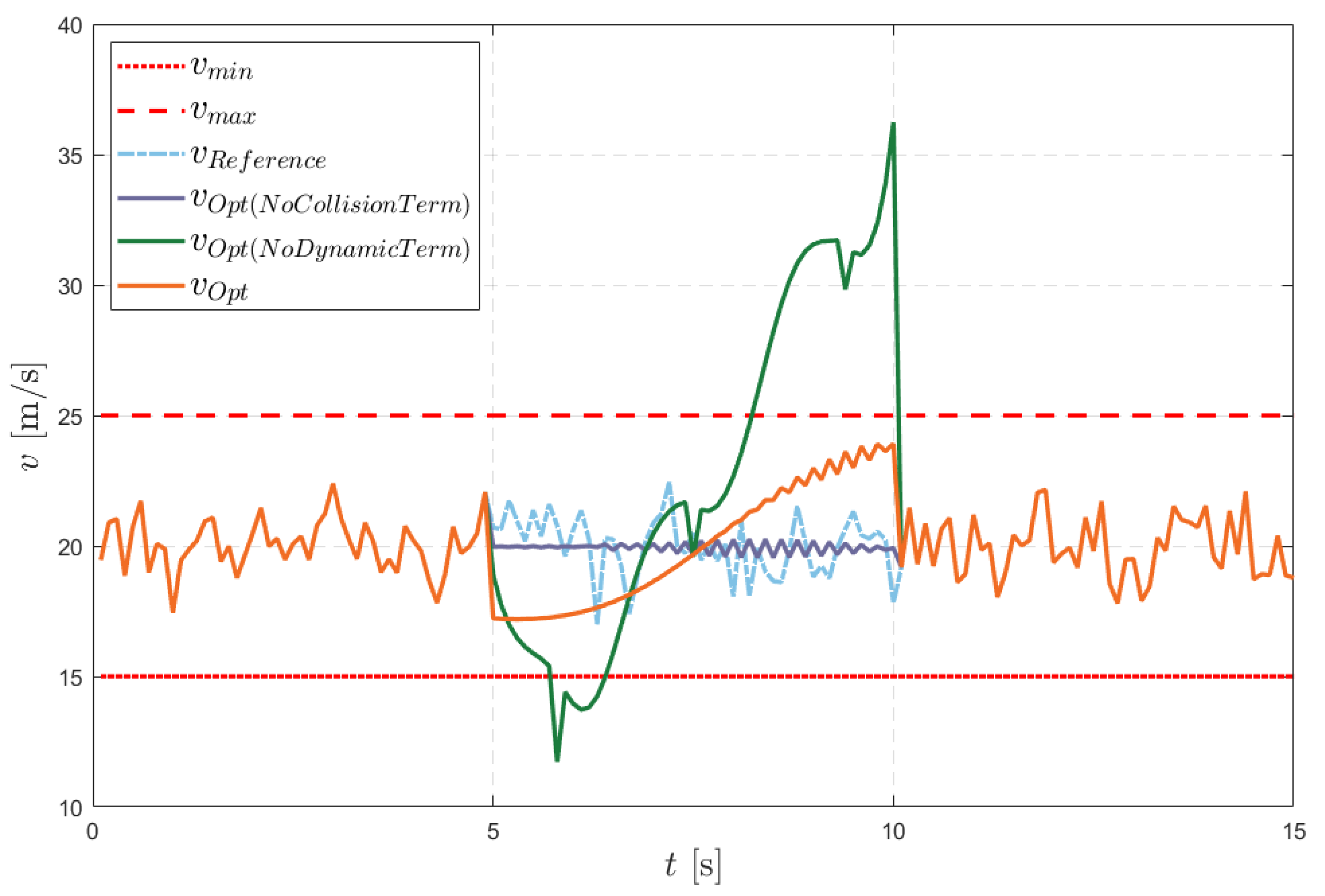
Next, we evaluate the effectiveness of our gradient-based trajectory replanning optimization. In the simulation, the moving obstacle starts from the state ${[0,0,0]}^T$ with a velocity of $20\mathrm{m}/\mathrm{s}$ and a turn rate of $-0.2\mathrm{rad}/\mathrm{s}$. As in previous cases, random noise is introduced to both the obstacle’s velocity and turn rate throughout its motion. The reference trajectory begins from the state ${[140,45,-2.24]}^T$, with a velocity of $20\mathrm{m}/\mathrm{s}$ and a turn rate of $0.1\mathrm{rad}/\mathrm{s}$. In this scenario, a collision with the moving obstacle is imminent if the UAV does not replan its trajectory. We set the parameters ${\lambda }_s={\lambda }_c={\lambda }_d={\lambda }_k=1$, ${\lambda }_r=0.01$, ${\alpha }_c={\alpha }_v={\alpha }_{\omega }=0.1$, and $M_s=M_r=I_3$. Using our fusion prediction method, we predict the moving obstacle’s future position over the next 5 s and optimize our local trajectory based on these predictions.

Trajectory replanning optimization is performed at the 5 s mark. The current waypoint serves as the starting point of the replanned trajectory, while the waypoint 5 s ahead serves as the end point. The results, illustrated in Figure 3, show that our approach yields the most accurate results. The red path represents the reference trajectory, and the orange path represents the replanned trajectory, which successfully avoids the moving obstacle based on the current predictions. Additionally, we present the distance between the moving obstacle and the UAV in Figure 4, along with the UAV’s speed and turn rate in Figure 5 and Figure 6, respectively. As shown in these figures, our replanned trajectory consistently maintains a safe distance from the moving obstacle, while the airspeed and turn rate remain within the UAV’s physical limits.

To further validate the safety and dynamic feasibility of our algorithm, and to understand the contribution of its different components, we performed an ablation study by individually removing the collision term and dynamic term from the optimization process. The results of this study are also shown in Figure 3, Figure 4, Figure 5 and Figure 6. It is evident that, without the collision term, the distance between the UAV and the obstacle falls below the safe threshold. In contrast, without the dynamic term, the trajectory maintains a safe distance but fails to keep the speed and turn rate within the UAV’s physical limits, leading to a dynamically infeasible trajectory. This ablation study highlights the importance of each component of our algorithm, demonstrating its overall efficiency and effectiveness.

Furthermore, we evaluated whether the proposed algorithm can ensure UAV safety in the presence of multiple moving obstacles. During the process of avoiding the first obstacle, a second obstacle was detected. This prompted a second round of online trajectory optimization, where the avoidance of both moving obstacles was considered. The optimized trajectory is shown in Figure 7, where the black trajectory represents the result after the second replanning. As seen, the UAV successfully avoided both the first and second obstacles. The distance between the two moving obstacles and the UAV is illustrated in Figure 8, further demonstrating the effectiveness and safety of our algorithm.

4. Discussion

In the previous sections, we introduced the integration of the CVM and KMP to provide a comprehensive obstacle prediction system. The fusion prediction results are then used as a reference for trajectory replanning, where we design an appropriate cost function for online trajectory optimization to avoid moving obstacles.

We believe that motion prediction plays a critical role in motion planning. Therefore, we explored the integration of prediction and planning to ensure both the safety and intelligence of the system. In [31], the CVM is evaluated as a simple yet effective baseline method, while in [32], the KMP is introduced as a powerful imitation learning approach. Based on these insights, we combined the strengths of both methods to offer a fusion prediction approach. However, it is important to recognize that motion prediction is a complex task, and accurate prediction under all conditions remains challenging. Improving prediction accuracy requires incorporating more environmental clues, which is a direction we intend to explore further.

Regarding gradient-based trajectory optimization, this method has demonstrated high effectiveness [17,18,19]. In this study, we focus specifically on online trajectory replanning for fixed-wing UAVs. We designed a cost function that integrates the motion prediction results into a collision cost function. After experimenting with various forms of cost functions, we selected the current exponential function due to its smoothness characteristics. Additionally, we developed a dynamic feasibility cost function and a kinematic constraint cost function tailored to fixed-wing UAVs. To our knowledge, the kinematic constraint cost function we proposed has not been addressed in the previous literature, though the reference trajectory cost function and smoothness cost function are widely used.

The UAV parameters presented in this paper include minimum and maximum speeds of 15 m/s and 25 m/s, respectively, and a maximum turn rate of 1 rad/s. These parameters correspond to a small fixed-wing UAV with a wing area of 0.5 m² and a mass of 2 kg, powered by an electric motor with approximately 500 W, which provides no less than 6 N of thrust. This configuration is designed for light payloads and short-range missions, ensuring stable flight performance as well as reliable takeoff and landing capabilities.

In terms of safety distance, we believe that 10 m is a reasonable setting, especially in open areas or when supported by adequate perception and control systems. The safety distance is intended to maintain a minimum buffer between the UAV and other objects (such as the ground, obstacles, or other aircraft) to avoid collisions, turbulence, or other potential risks. For a fixed-wing UAV flying at the specified speeds, both its flight path and reaction time require some buffer space. And the 10-meter safety distance serves as a buffer against sudden obstacle appearances and aids in trajectory planning, rather than being relied upon solely for a full stop.

5. Conclusions

We have proposed an efficient online trajectory replanning algorithm for fixed-wing UAVs that integrates predictions of moving obstacles into a gradient-based trajectory optimization framework. Our simulations demonstrate that this method performs well in dynamic environments, effectively helping UAVs avoid moving obstacles.

Our motion prediction method demonstrated promising results in the experiments; however, it should be noted that its performance is not consistently good across all scenarios. In future research, we will focus on enhancing the accuracy of long-term trajectory predictions by integrating additional contextual information, such as the interactions between the UAV and other dynamic agents in the environment. This will enable more robust and reliable decision-making in complex scenarios. Moreover, we plan to incorporate Model Predictive Control (MPC) into our optimization framework. This integration aims to address the challenges of effective UAV navigation in highly dynamic environments, where rapid adaptation to changing conditions is critical for maintaining safety and efficiency.