
Wasserstein-Based Evolutionary Operators for Optimizing Sets of Points: Application to Wind-Farm Layout Design

 ,
,
Abstract
1. Introduction and Related Work
1.1. General Context
1.2. Related Work
1.2.1. Mathematical Programming Techniques
1.2.2. Evolutionary and Other Stochastic Algorithms
1.3. Contribution of This Work
- A cloud of continuous vectors can be modeled as a uniform discrete measure with finite support.
- This model helps defining a topology in the space of clouds of points using the Wasserstein distance between measures.
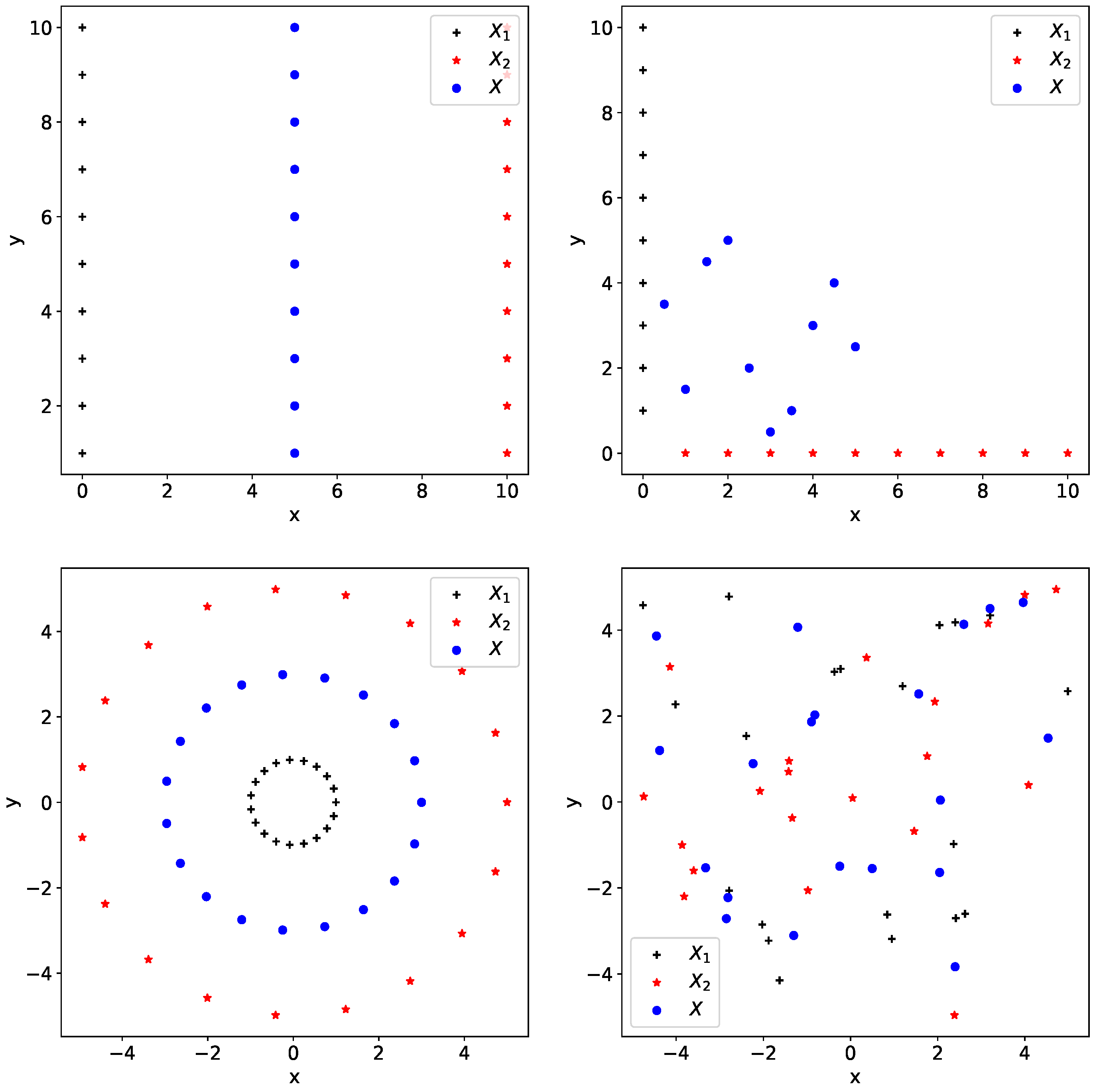
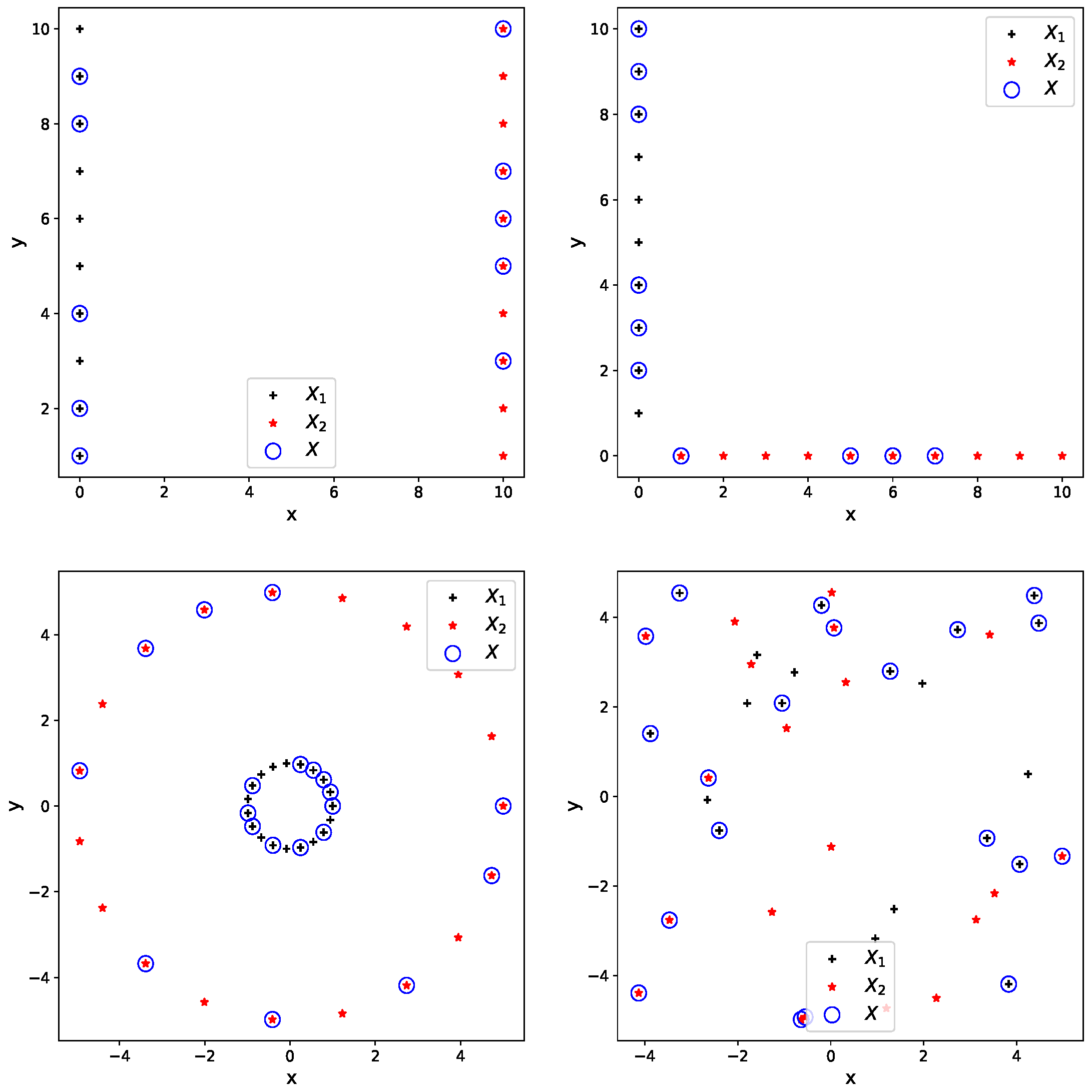
- We propose evolutionary crossover and mutation operators relying on the concept of the Wasserstein barycenter.
2. Wasserstein Barycenters for the Evolutionary Optimization of Sets
| Algorithm 1 Structure of the ES-() Algorithm |
Input: the population size, the number of iterations, F a function defined over clouds of points, Output: the best cloud of points found and its fitness value;
|
2.1. Fréchet Mean to Wasserstein Barycenter
- corresponds to the Euclidean distance between and
- is the set of all probability measures defined over with marginals μ and ν.
- ,
- ,
- ,
- If the above is verified, we have
2.2. Wasserstein-Based Crossover and Mutation Operators
2.2.1. Crossover
- Equal weight crossover: taketo be a new design.
- Random weight crossover: draw random and consideras a new design.
- If , then
- Otherwise, if , generate two crossovers, and , with and
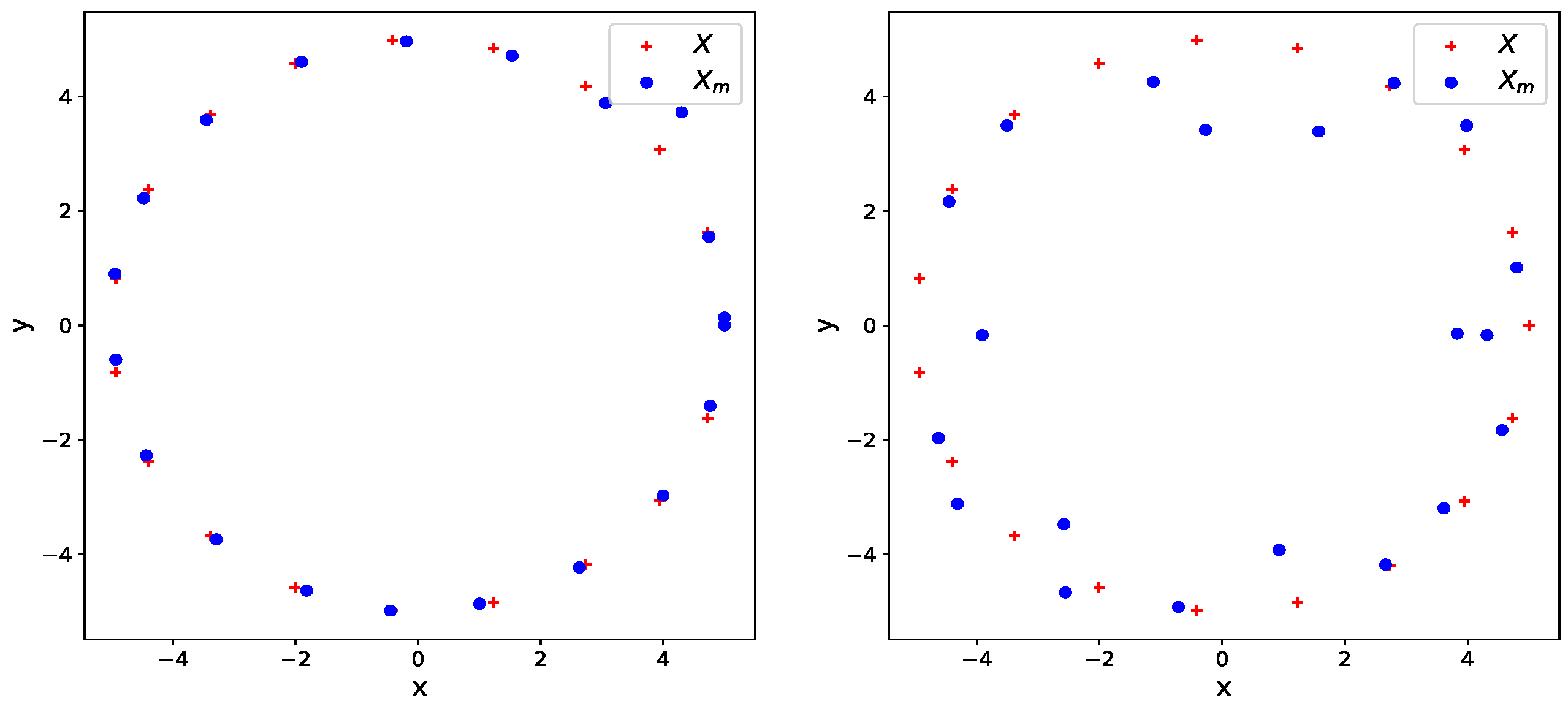
2.2.2. Mutation
- in the space of all possible sizes: full size choice
- in with : ternary size choice.
- The weight is uniformly random, whereas Levy flights jumps occur deterministically in case of prolonged stagnation.
- In the space of clouds, the boundary mutation is focused towards expanding the cloud of points, which is a design choice meant to counteract the effect of crossover, whereas the Levy flights have no preferential direction of perturbation.
2.3. An Alternating Mutation
| Algorithm 2 Alternating Wasserstein mutation |
Input: X cloud to mutate, prob the probability to perform a Boundary mutation Output: The mutated cloud(s)
|
2.4. Successive Boundary and Full Domain Mutations
2.4.1. Successive Mutations with Independent Random Weights
| Algorithm 3 Independently Weighted (Wasserstein) mutation |
Input: X cloud to mutate Output: The mutated cloud(s);
|
2.4.2. Successive Mutations with a Single Random Weight
| Algorithm 4 Uniquely Weighted (Wasserstein) mutation |
Input: X cloud to mutate Output: The mutated cloud(s);
|
3. Numerical Analysis
3.1. A Classical Evolutionary Algorithm Applied to Sets
3.1.1. Baseline Algorithm Encoding and Crossover
| Algorithm 5 Uniform crossover between sequences |
Input: and Output: their crossover
|
3.1.2. Mutation
| Algorithm 6 Gaussian mutation |
Input: , Output: A mutation of X
|
3.2. Experimental Protocol
3.2.1. Algorithms Settings
- We consider square search domains. The length of each side is 100.
- A discretization of step 1 is applied to each side for the sampling on the boundaries for boundary mutation. Continuous alternatives, however, should also work.
- , , .
- The population size is set equal to 10 times the average number of active components in each set, = 300, and the maximum number of iterations of the algorithms is .
- Regarding the choice of , we consider it proportional to , where X and are points sampled uniformly in the domain. The latter quantity is the mean squared distance between two points sampled uniformly in the domain. In a centered-squared domain of side L, we obtain with , the variance of a uniform continuous law. In our case, .
- The default value of prob (Algorithm 2), if not specified, is 0.5.
3.2.2. Performance Metrics
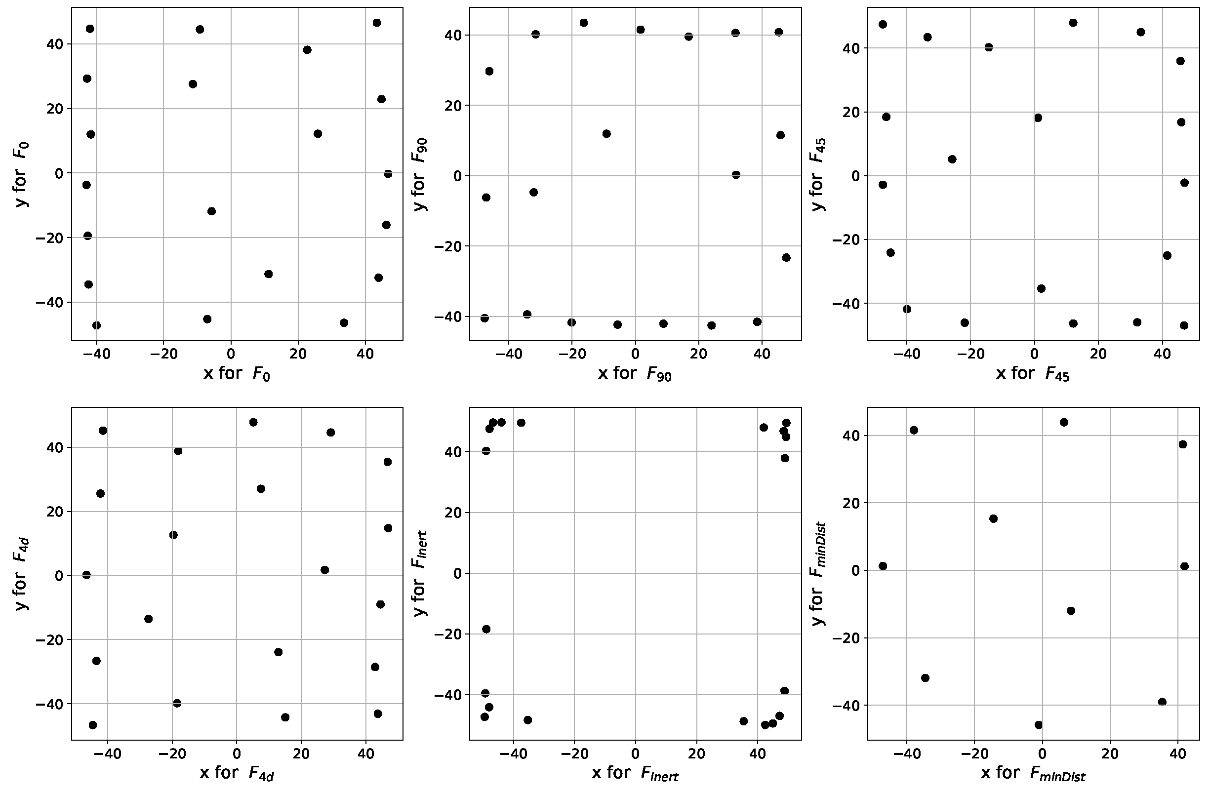
3.3. Analytical Test Functions
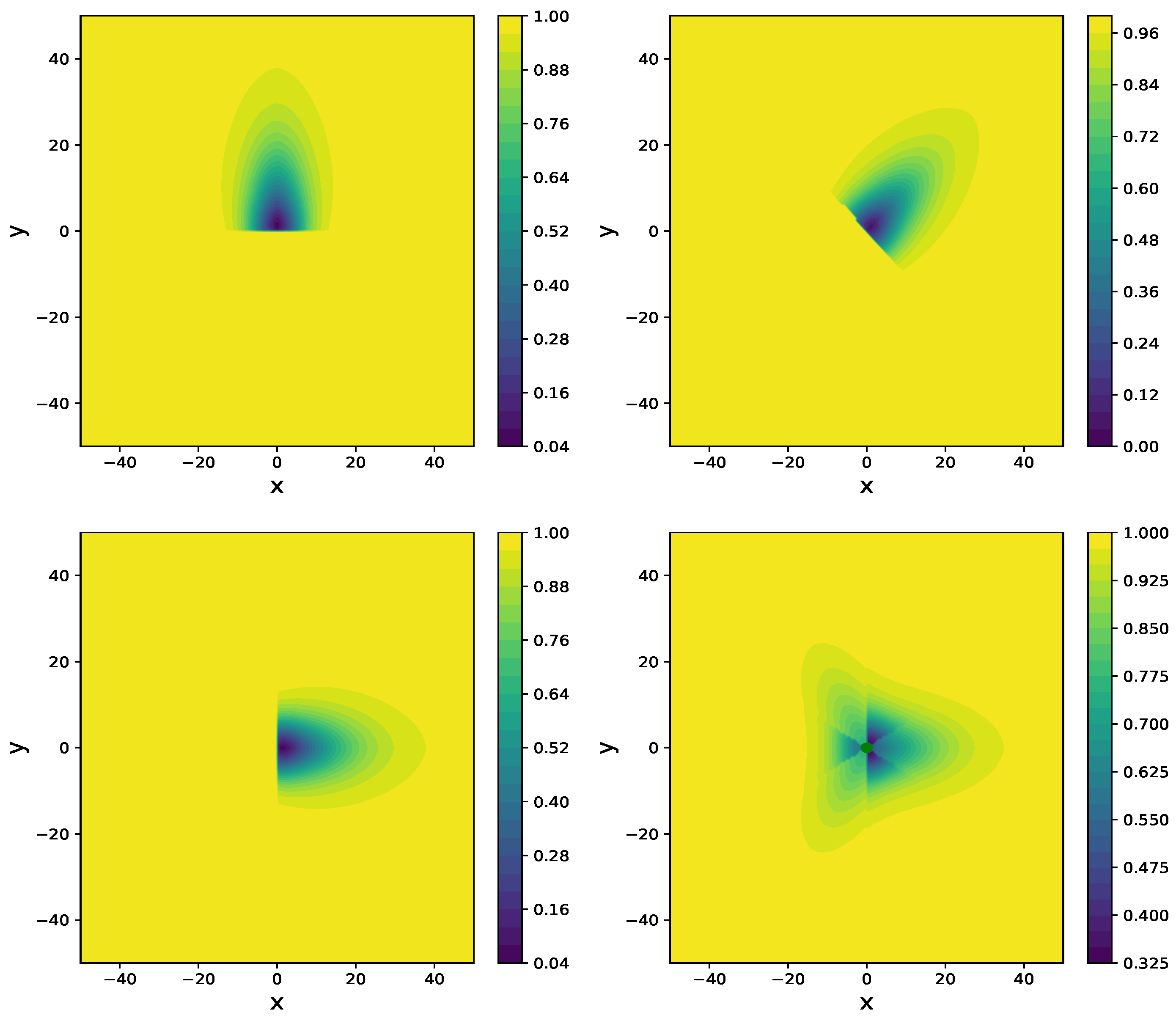
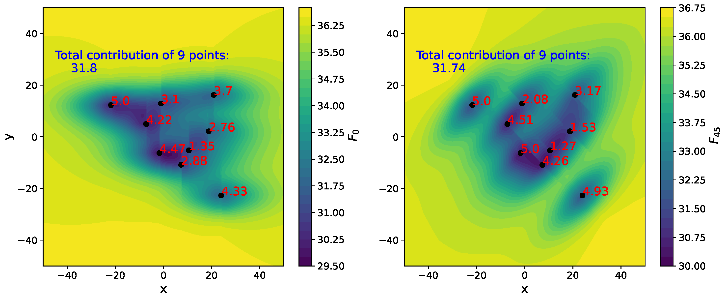
3.3.1. Wind Farm Proxy
- stands for functions that account for wind coming from a single direction .
- stands for functions modeling the average effect of n wind directions chosen in .
3.3.2. MinDist Function
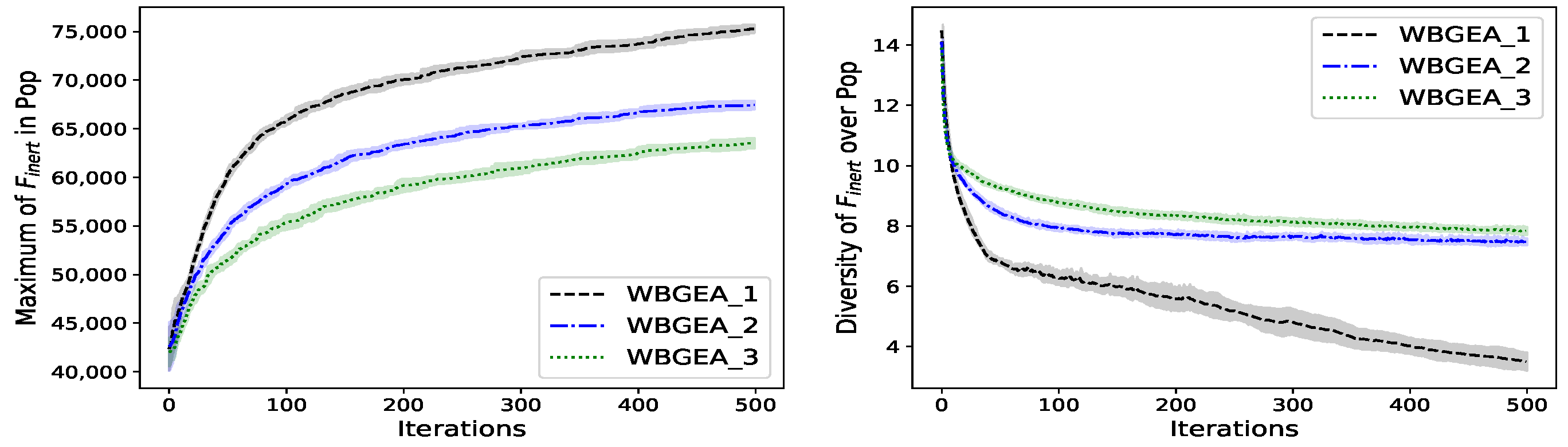
3.3.3. Inertia Function
3.4. Designs Returned by the Algorithm WBGEA_1t_nc
4. Results and Discussions
4.1. Study of a Wasserstein-Based Evolutionary Algorithm
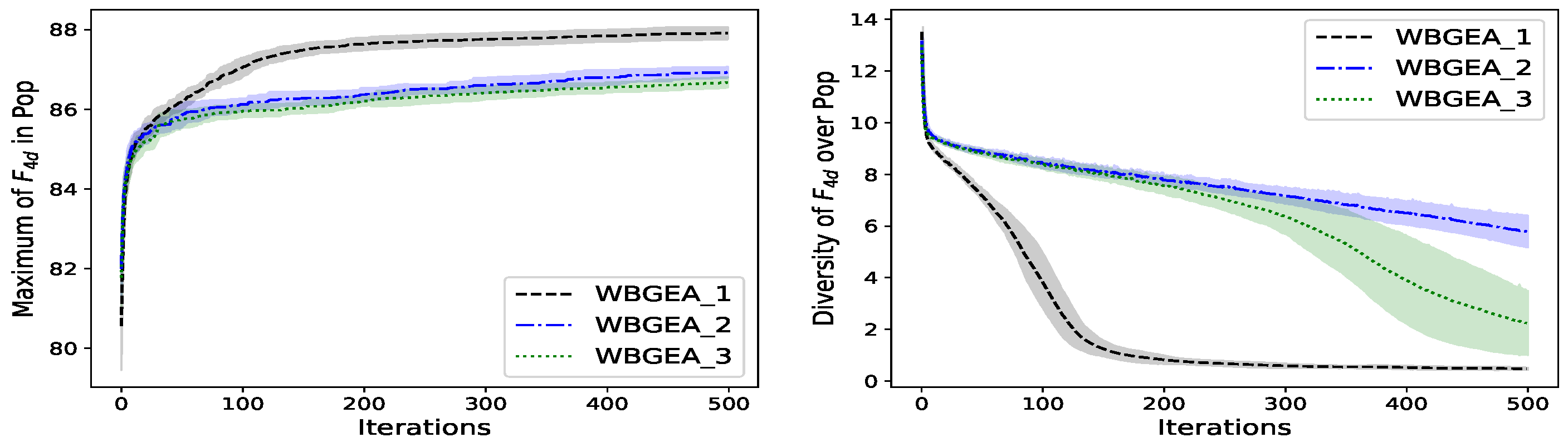
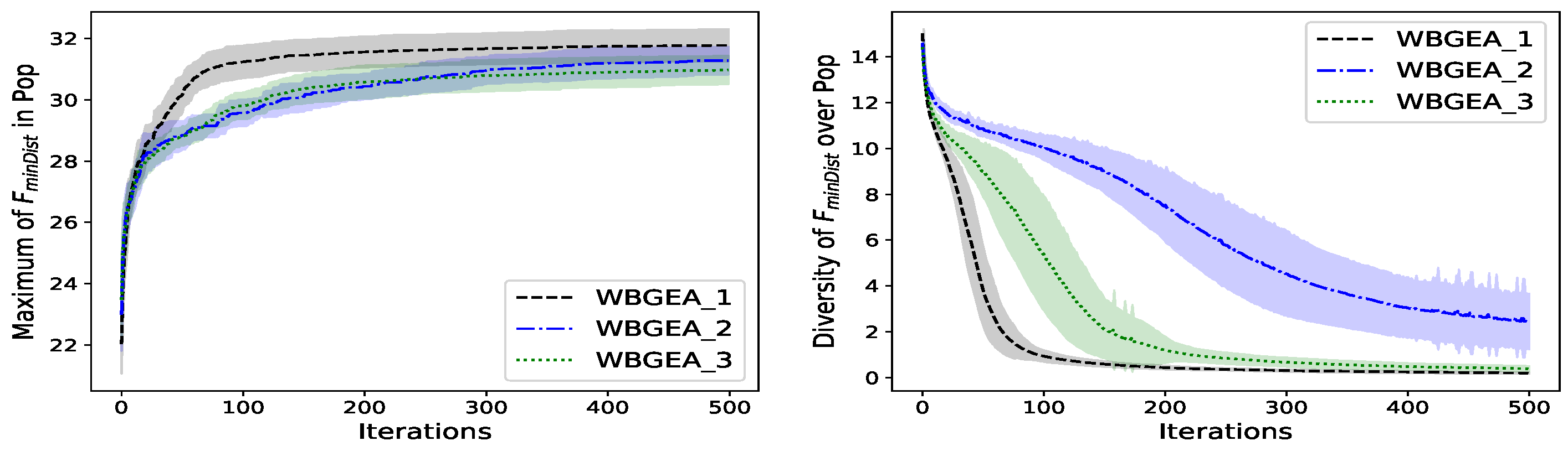
4.1.1. Alternating vs. Successive Boundary and Full Domain Mutations
4.1.2. Handling of Set Size in Mutation: Ternary vs. Full Size
4.2. Comparison of Wasserstein and Sequence-Based Operators
4.2.1. Wasserstein-Based vs. Reference Evolutionary Algorithm
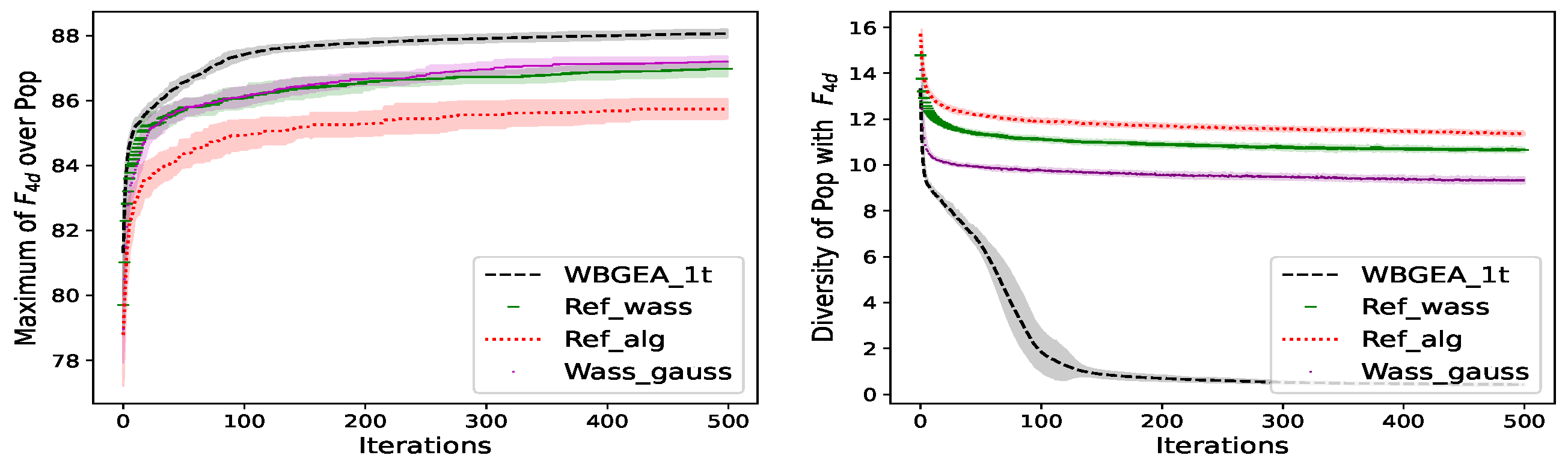
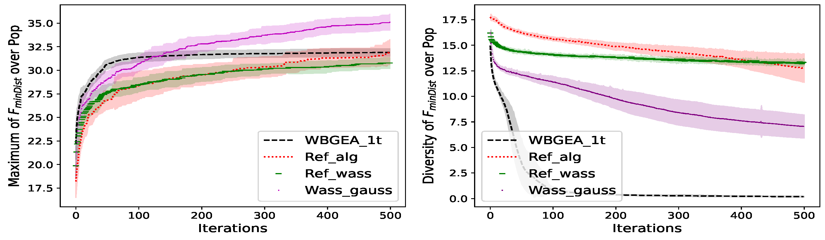
4.2.2. Wasserstein vs. Classical Evolutionary Operators
4.3. Investigating the Role of the Mutation and the Crossover
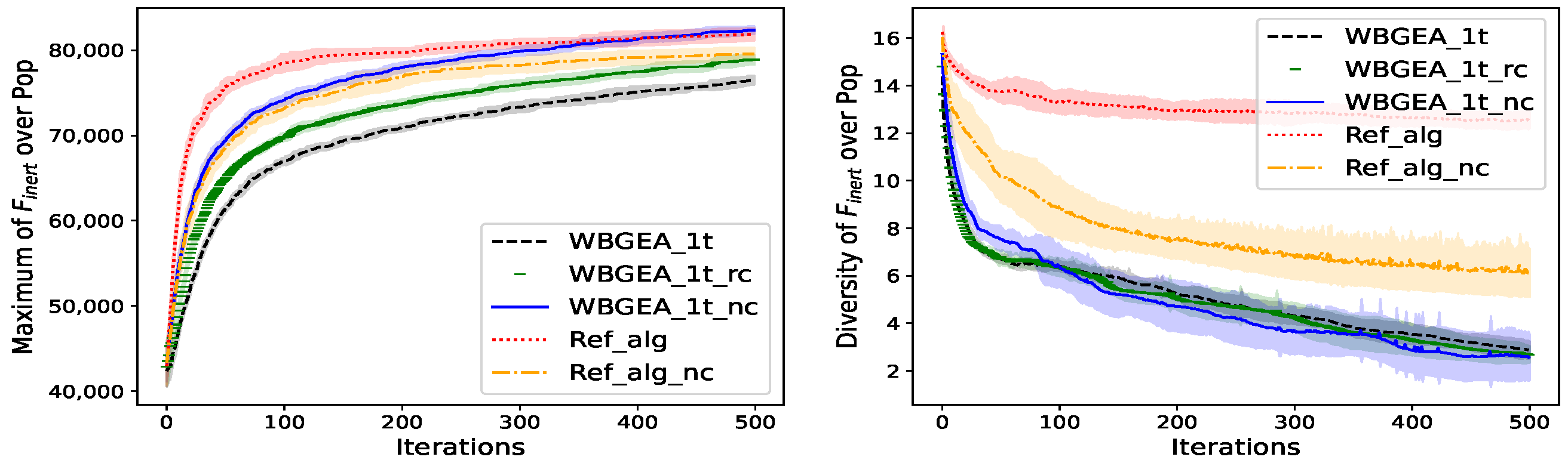
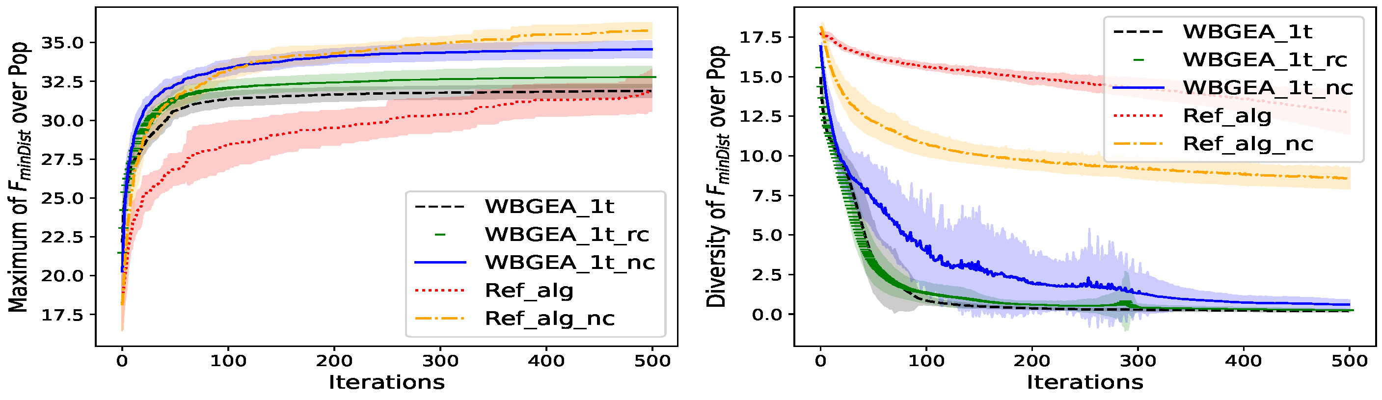
4.3.1. Role of Crossover
- Relaxed Crossover
- Absence of Crossover
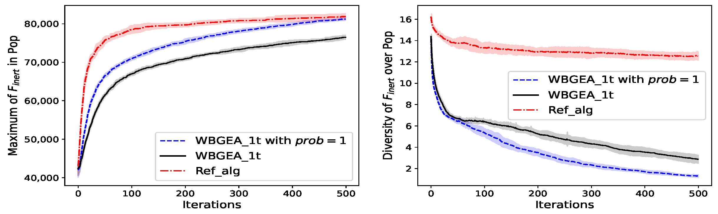
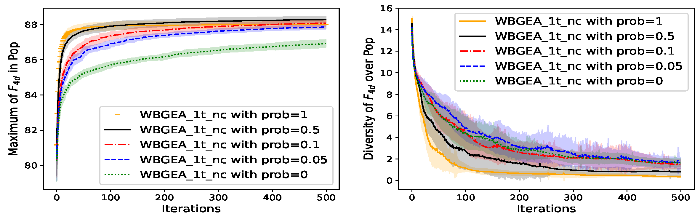
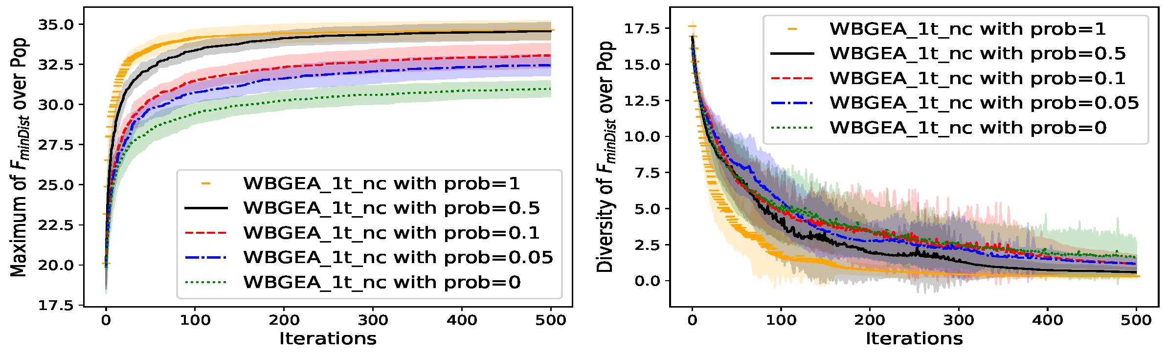
4.3.2. Role of the Boundary Mutation
4.4. Synthesis
4.4.1. Wasserstein-Based Operators
4.4.2. The Test Suite
4.4.3. On the Random Choice of Operators
4.4.4. Population Diversity: Summary of Results and Visualization
5. Conclusions and Perspectives
Author Contributions
Funding
Institutional Review Board Statement
Informed Consent Statement
Data Availability Statement
Conflicts of Interest
Abbreviations
| d | Dimension of a vector |
| A compact subset of | |
| The diversity of pop, a population of sets | |
| n, | Size of sets of vectors |
| prob | Probability to perform a boundary mutation |
| A measure associated with a set of points X | |
| The set of discrete measures with finite support | |
| Dirac function | |
| Gaussian mutation variance | |
| Set of n unordered points where and . It will be referred to as a cloud, set or bag of points (or vectors). Compared to an (ordered) list of points, X is invariant with respect to any point permutation because it is a set. | |
| Number of vectors in X |
Appendix A. Proof That the Wasserstein Barycenter Is Contracting
Appendix B. Handling of Set Size in Mutation: Supplementary Results

Appendix C. Details about Wind Farm Proxy
References
- Larsen, G.C.; Réthoré, P.E. TOPFARM—A tool for wind farm optimization. Energy Procedia 2013, 35, 317–324. [Google Scholar] [CrossRef]
- Mosetti, G.; Poloni, C.; Diviacco, B. Optimization of wind turbine positioning in large windfarms by means of a genetic algorithm. J. Wind Eng. Ind. Aerodyn. 1994, 51, 105–116. [Google Scholar] [CrossRef]
- Kusiak, A.; Song, Z. Design of wind farm layout for maximum wind energy capture. Renew. Energy 2010, 35, 685–694. [Google Scholar] [CrossRef]
- Cazzaro, D.; Pisinger, D. Variable neighborhood search for large offshore wind farm layout optimization. Comput. Oper. Res. 2022, 138, 105588. [Google Scholar] [CrossRef]
- Amorosi, L.; Fischetti, M.; Paradiso, R.; Roberti, R. Optimization models for the installation planning of offshore wind farms. Eur. J. Oper. Res. 2024, 315, 1182–1196. [Google Scholar] [CrossRef]
- Zhong, J.; Li, Y.; Wu, Y.; Cao, Y.; Li, Z.; Peng, Y.; Qiao, X.; Xu, Y.; Yu, Q.; Yang, X.; et al. Optimal operation of energy hub: An integrated model combined distributionally robust optimization method with Stackelberg game. IEEE Trans. Sustain. Energy 2023, 14, 1835–1848. [Google Scholar] [CrossRef]
- Bauer, J.; Lysgaard, J. The offshore wind farm array cable layout problem: A planar open vehicle routing problem. J. Oper. Res. Soc. 2015, 66, 360–368. [Google Scholar] [CrossRef]
- Alarie, S.; Audet, C.; Garnier, V.; Le Digabel, S.; Leclaire, L. Snow water equivalent estimation using blackbox optimization. Pac. J. Optim. 2013, 9, 1–21. [Google Scholar]
- Chaloner, K.; Verdinelli, I. Bayesian Experimental Design: A Review. Stat. Sci. 1995, 10, 273–304. [Google Scholar] [CrossRef]
- Stenger, J. Optimal Uncertainty Quantification of a Risk Measurement from a Computer Code. Ph.D. Thesis, Université Paul Sabatier-Toulouse III, Toulouse, France, 2020. [Google Scholar]
- McLachlan, G.J.; Basford, K.E. Mixture Models. Inference and Applications to Clustering; M. Dekker: New York, NY, USA, 1988. [Google Scholar]
- Eiben, A.E.; Smith, J.E. Introduction to Evolutionary Computing; Springer: Berlin/Heidelberg, Germany, 2015. [Google Scholar]
- Hansen, N.; Arnold, D.V.; Auger, A. Evolution Strategies. In Handbook of Computational Intelligence; Kacprzyk, J., Pedrycz, W., Eds.; Number 871-898; Springer: Berlin/Heidelberg, Germany, 2015. [Google Scholar]
- Pérez, B.; Mínguez, R.; Guanche, R. Offshore wind farm layout optimization using mathematical programming techniques. Renew. Energy 2013, 53, 389–399. [Google Scholar] [CrossRef]
- Byrd, R.H.; Nocedal, J.; Waltz, R.A. K nitro: An integrated package for nonlinear optimization. In Large-Scale Nonlinear Optimization; Springer: Boston, MA, USA, 2006; pp. 35–59. [Google Scholar]
- Fagerfjäll, P. Optimizing Wind Farm Layout: More Bang for the Buck Using Mixed Integer Linear Programming. Master’s Thesis, Chalmers University of Technology and Gothenburg University, Göteborg, Sweden, 2010. Volume 111. [Google Scholar]
- Fischetti, M.; Pisinger, D. Mathematical optimization and algorithms for offshore wind farm design: An overview. Bus. Inf. Syst. Eng. 2019, 61, 469–485. [Google Scholar] [CrossRef]
- Kim, J. Cardinality Constrained Optimization Problems. Ph.D. Dissertation, Purdue University, West Lafayette, IN, USA, 2016. [Google Scholar]
- Surry, P.D.; Radcliffe, N.J. Formal search algorithms + problem characterisations = executable search strategies. In Theory and Principled Methods for the Design of Metaheuristics; Springer: Berlin/Heidelberg, Germany, 2013; pp. 247–270. [Google Scholar]
- Michalewicz, Z. Genetic Algorithms + Data Structures = Evolution Programs; Springer Science & Business Media: Berlin/Heidelberg, Germany, 1996. [Google Scholar]
- Radcliffe, N.J. Genetic Set Recombination. In Foundations of Genetic Algorithms; Whitley, L.D., Ed.; Elsevier: Amsterdam, The Netherlands, 1993; Volume 2, pp. 203–219. [Google Scholar] [CrossRef]
- Eroğlu, Y.; Seçkiner, S.U. Design of wind farm layout using ant colony algorithm. Renew. Energy 2012, 44, 53–62. [Google Scholar] [CrossRef]
- Feng, J.; Shen, W.Z. Solving the wind farm layout optimization problem using random search algorithm. Renew. Energy 2015, 78, 182–192. [Google Scholar] [CrossRef]
- Bilbao, M.; Alba, E. Simulated annealing for optimization of wind farm annual profit. In Proceedings of the 2009 2nd International Symposium on Logistics and Industrial Informatics, Linz, Austria, 10–12 September 2009; IEEE: Piscataway, NJ, USA, 2009; pp. 1–5. [Google Scholar]
- Grady, S.; Hussaini, M.; Abdullah, M.M. Placement of wind turbines using genetic algorithms. Renew. Energy 2005, 30, 259–270. [Google Scholar] [CrossRef]
- Réthoré, P.E.; Fuglsang, P.; Larsen, G.C.; Buhl, T.; Larsen, T.J.; Madsen, H.A. TOPFARM: Multi-fidelity optimization of wind farms. Wind Energy 2014, 17, 1797–1816. [Google Scholar] [CrossRef]
- Arora, J.S. Introduction to Optimum Design; Elsevier: Amsterdam, The Netherlands, 2004. [Google Scholar]
- Goldberg, D. Genetic Algorithms in Search, Optimization and Machine Learning; Addion Wesley: Reading, MA, USA, 1989. [Google Scholar]
- Song, S.; Li, Q.; Felder, F.A.; Wang, H.; Coit, D.W. Integrated optimization of offshore wind farm layout design and turbine opportunistic condition-based maintenance. Comput. Ind. Eng. 2018, 120, 288–297. [Google Scholar] [CrossRef]
- Pillai, A.C.; Chick, J.; Johanning, L.; Khorasanchi, M.; Pelissier, S. Optimisation of offshore wind farms using a genetic algorithm. Int. J. Offshore Polar Eng. 2016, 26, 225–234. [Google Scholar] [CrossRef]
- Pillai, A.C.; Chick, J.; Johanning, L.; Khorasanchi, M.; Barbouchi, S. Comparison of offshore wind farm layout optimization using a genetic algorithm and a particle swarm optimizer. In Proceedings of the International Conference on Offshore Mechanics and Arctic Engineering, Busan, Republic of Korea, 19–24 June 2016; Volume 49972, p. V006T09A033. [Google Scholar]
- Villani, C. Optimal Transport: Old and New; Springer: Berlin/Heidelberg, Germany, 2009; Volume 338. [Google Scholar]
- Sloss, A.N.; Gustafson, S. 2019 evolutionary algorithms review. arXiv 2019, arXiv:1906.08870. [Google Scholar]
- Bartz-Beielstein, T.; Branke, J.; Mehnen, J.; Mersmann, O. Evolutionary algorithms. Wiley Interdiscip. Rev. Data Min. Knowl. Discov. 2014, 4, 178–195. [Google Scholar] [CrossRef]
- Cao, X. Poincaré Fréchet mean. Pattern Recognit. 2023, 137, 109302. [Google Scholar] [CrossRef]
- Montrucchio, L.; Pistone, G. Kantorovich distance on a finite metric space. arXiv 2019, arXiv:1905.07547. [Google Scholar]
- Cuturi, M.; Doucet, A. Fast computation of Wasserstein barycenters. In Proceedings of the International Conference on Machine Learning, PMLR, Beijing, China, 22–24 June 2014; pp. 685–693. [Google Scholar]
- Flamary, R.; Courty, N.; Gramfort, A.; Alaya, M.Z.; Boisbunon, A.; Chambon, S.; Chapel, L.; Corenflos, A.; Fatras, K.; Fournier, N.; et al. Pot: Python optimal transport. J. Mach. Learn. Res. 2021, 22, 1–8. [Google Scholar]
- Agueh, M.; Carlier, G. Barycenters in the Wasserstein space. SIAM J. Math. Anal. 2011, 43, 904–924. [Google Scholar] [CrossRef]
- Haklı, H.; Uğuz, H. A novel particle swarm optimization algorithm with Levy flight. Appl. Soft Comput. 2014, 23, 333–345. [Google Scholar] [CrossRef]
- Sebag, M.; Ducoulombier, A. Extending population-based incremental learning to continuous search spaces. In Proceedings of the Parallel Problem Solving from Nature—PPSN V, Amsterdam, The Netherlands, 27–30 September 1998; Eiben, A.E., Bäck, T., Schoenauer, M., Schwefel, H.P., Eds.; Springer: Berlin/Heidelberg, Germany, 1998; pp. 418–427. [Google Scholar]
- Hansen, N. The CMA evolution strategy: A comparing review. In Towards a New Evolutionary Computation: Advances in the Estimation of Distribution Algorithms; Springer: Berlin/Heidelberg, Germany, 2006; pp. 75–102. [Google Scholar]
- Santner, T.J.; Williams, B.J.; Notz, W.I.; Williams, B.J. The Design and Analysis of Computer Experiments; Springer: New York, NY, USA, 2003; Volume 1. [Google Scholar]
- Hansen, N.; Ros, R.; Mauny, N.; Schoenauer, M.; Auger, A. Impacts of invariance in search: When CMA-ES and PSO face ill-conditioned and non-separable problems. Appl. Soft Comput. 2011, 11, 5755–5769. [Google Scholar] [CrossRef]
- Jansen, T.; Wegener, I. Real royal road functions-where crossover provably is essential. Discret. Appl. Math. 2005, 149, 111–125. [Google Scholar] [CrossRef]
- Consoli, P.A.; Mei, Y.; Minku, L.L.; Yao, X. Dynamic selection of evolutionary operators based on online learning and fitness landscape analysis. Soft Comput. 2016, 20, 3889–3914. [Google Scholar] [CrossRef]
- El, N.; Hassan, H. Topologie Générale et Espaces Normés; ZI des Hauts, no. Édition, 54692; Dunod: Malakoff, France, 2011. [Google Scholar]
- Paty, F.P.; Cuturi, M. Subspace robust Wasserstein distances. In Proceedings of the International Conference on Machine Learning, PMLR, Long Beach, CA, USA, 9–15 June 2019; pp. 5072–5081. [Google Scholar]


| Algorithm | Crossover | Mutation |
|---|---|---|
| WBGEA_1 | Equal Weight crossover (Equation (2)) | Alternating mutation (Algorithm 2). Full size choice (Definition 5). |
| WBGEA_2 | Equal Weight crossover (Equation (2)) | Successive independently weighted mutation (Algorithm 3). Full size choice (Definition 5). |
| WBGEA_3 | Equal Weight crossover (Equation (2)) | Successive equally weighted mutation (Algorithm 4). Full size choice (Definition 5). |
| WBGEA_1t (t for ternary) | Equal Weight crossover (Equation (2)) | Alternating mutation (Algorithm 2). Ternary size choice (Definition 5). |
| WBGEA_1t_nc (nc for no crossover) | No crossover | Alternating mutation (Algorithm 2). Ternary size choice (Definition 5). |
| WBGEA_1t_rc (rc for random weight in crossover) | Random Weight crossover (Equation (3)) | The mutation is carried out with Algorithm 2. Ternary size choice (Definition 5). |
| Ref_alg | Uniform crossover on sequences (Algorithm 5) | Gaussian mutation (Algorithm 6) |
| Ref_alg_nc | No crossover | Gaussian mutation (Algorithm 6) |
| Ref_wass | Uniform crossover on sequences (Algorithm 5) | Alternating mutation (Algorithm 2). Ternary size choice (Definition 5). |
| Wass_gauss | Equal Weight crossover (Equation (2)) | Gaussian mutation (Algorithm 6) |
| Experiments | Compared Algorithms | The Scientific Questions |
|---|---|---|
| Alternating vs. successive Boundary and Full Domain mutations | WBGEA_1, WBGEA_2, WBGEA_3 | Are there major differences between the three mutations in WBGEA? |
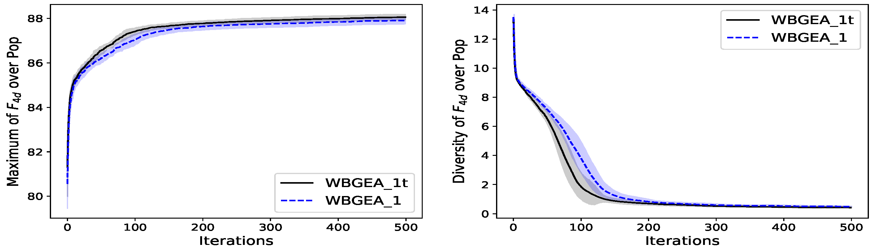
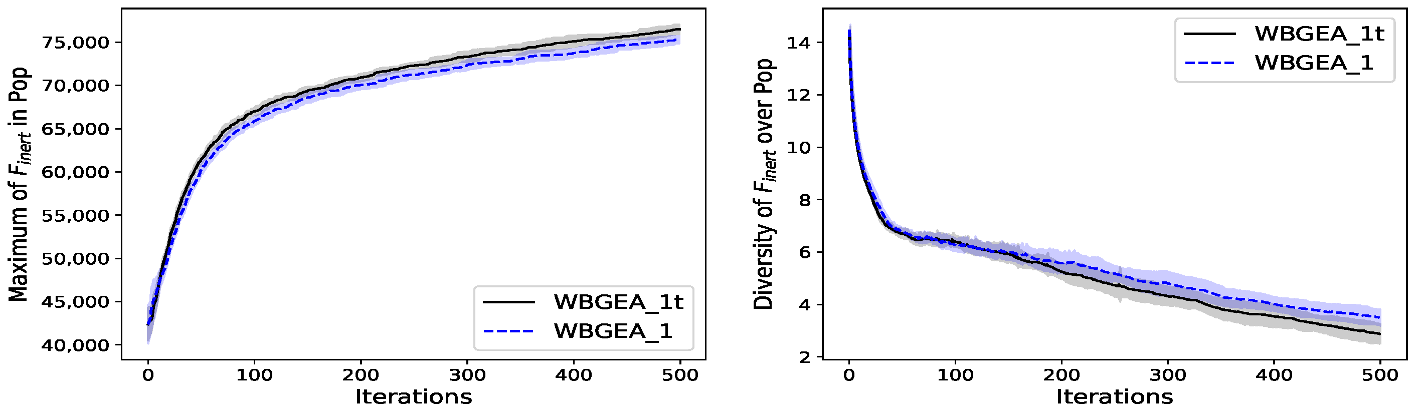
| Handling of set size in mutation: ternary vs. full size | WBGEA_1, WBGEA_1t | How does the size of affect the performances of the algorithms? |
| Wasserstein-based vs. reference evolutionary algorithm | WBGEA_1t, Ref_alg | How does the default Wasserstein-based evolutionary algorithm compare to a more classical evolutionary algorithm? |
| Wasserstein vs. classical evolution operators | WBGEA_1t, Ref_alg, Ref_wass, Wass_gauss | How do the different operators behave when composed together differently? |
| Role of crossover | WBGEA_1t, WBGEA_1t_rc, WBGEA_1t_nc, Ref_alg, Ref_alg_nc | Are there noticeable differences between the random and the equal weight crossovers in WBGEA? Does the crossover play a major role in the performance of the algorithms? |
| Role of the boundary mutation | WBGEA_1t_nc with four different prob: 1, 0.5, 0.1, 0.05 and 0 | What happens if we diminish the chances of performing a boundary mutation in the absence of crossover? |
| Algorithm | ||||||
|---|---|---|---|---|---|---|
| WBGEA_1 | 89.158 (±0.196) | 89.183 (±0.133) | 89.714 (±0.193) | 87.908 (±0.157) | 31.785 (±0.530) | 71,112 (±700) |
| WBGEA_2 | 88.147 (±0.148) | 88.279 (±0.139) | 88.704 (±0.112) | 86.936 (±0.137) | 31.279 (±0.455) | 67,451 (±462) |
| WBGEA_3 | 88.117 (±0.219) | 88.033 (±0.140) | 88.476 (±0.132) | 86.672 (±0.129) | 30.977 (±0.467) | 63,510 (±538) |
| WBGEA_1t | 89.270 (±0.163) | 89.334 (±0.154) | 89.872 (±0.208) | 87.908 (±0.157) | 31.892 (±0.404) | 76,480 (±566) |
| Ref_alg | 87.281 (±0.438) | 87.345 (±0.408) | 87.398 (±0.319) | 85.742 (±0.307) | 31.923 (±1.337) | 81,869 (±758) |
| Ref_alg_nc | 88.734 (±0.208) | 88.681 (±0.281) | 88.891 (±0.222) | 87.453 (±0.179) | 35.780 (±0.495) | 79,562 (±737) |
| Ref_wass | 88.938 (±0.293) | 89.036 (±0.378) | 88.906 (±0.265) | 86.974 (±0.228) | 30.769 (±0.572) | 94,211 (±616) |
| Wass_gauss | 88.430 (±0.242) | 88.383 (±0.257) | 88.667 (±0.191) | 87.199 (±0.166) | 35.108 (±0.857) | 79,116 (±1575) |
| WBGEA_1t_nc | 89.939 (±0.237) | 89.928 (±0.183) | 89.895 (±0.161) | 88.269 (±0.185) | 34.561 (±0.525) | 82,375 (±484) |
| WBGEA_1t_nc (prob = 1) | 89.879 (±0.251) | 89.823 (±0.211) | 89.952 (±0.231) | 87.997 (±0.220) | 34.635 (±0.578) | 85,947 (±625) |
| WBGEA_1t_nc (prob = 0.1) | 89.612 (±0.212) | 89.698 (±0.189) | 89.737 (±0.105) | 88.065 (±0.160) | 33.051 (±0.742) | 74,948 (±521) |
| WBGEA_1t_nc (prob = 0.05) | 89.346 (±0.205) | 89.399 (±0.216) | 89.438 (±0.111) | 87.846 (±0.113) | 32.447 (±.641) | 71,907 (±898) |
| WBGEA_1t_nc (prob = 0) | 88.195 (±0.201) | 88.166 (±0.182) | 88.316 (±0.124 | 86.921 (±0.216) | 30.986 (±0.491) | 51,306 (±1195) |
| WBGEA_1t_rc | 89.649 (±0.191) | 89.613 (±0.220) | 89.686 (±0.168) | 88.097 (±0.166) | 32.785 (±0.655) | 78,888 (±604) |
| Experiments | The Scientific Questions | Conclusions |
|---|---|---|
| Alternating vs. successive boundary and full domain mutations | Are there major differences between the three mutations in WBGEA? | Alternating Wasserstein mutation (Algorithm 2) yields the best results when coupled with equal weight crossover on all the functions. |
| Handling of sets size in mutation: ternary vs. full size choice | How does the size of affect the performance of the algorithms? | The two schemes for choosing the size of do not make a significant difference. |
| Wasserstein-based vs. reference evolutionary algorithm | How does the default Wasserstein-based evolutionary algorithm compare to a more classical evolutionary algorithm? | WBGEA, compared to Ref_alg, yields better results on wind-farm test functions and converges faster on . An adapted tuning helps to obtain similar results on . |
| Wasserstein vs. classical evolution operators | How do the different operators behave when composed together differently? | Wasserstein-based operators improve over sequence-based operators on all the test functions but . |
| Role of crossover | Are there noticeable differences between the random and the equal weight crossovers in WBGEA ? Does the crossover play a major role in the performance of the algorithms? | WBGEA with random weight crossover (Equation (3)) improves over equal weight, but removing the crossover is an even better choice. |
| Role of the boundary mutation | What happens if we diminish the chances of performing a Boundary mutation in the absence of crossover? | High values of the boundary mutation probability (around 0.5) are adapted to the tested suite of functions. |
Disclaimer/Publisher’s Note: The statements, opinions and data contained in all publications are solely those of the individual author(s) and contributor(s) and not of MDPI and/or the editor(s). MDPI and/or the editor(s) disclaim responsibility for any injury to people or property resulting from any ideas, methods, instructions or products referred to in the content. |
© 2024 by the authors. Licensee MDPI, Basel, Switzerland. This article is an open access article distributed under the terms and conditions of the Creative Commons Attribution (CC BY) license (https://creativecommons.org/licenses/by/4.0/).
Share and Cite
Sow, B.; Le Riche, R.; Pelamatti, J.; Keller, M.; Zannane, S. Wasserstein-Based Evolutionary Operators for Optimizing Sets of Points: Application to Wind-Farm Layout Design. Appl. Sci. 2024, 14, 7916. https://doi.org/10.3390/app14177916
Sow B, Le Riche R, Pelamatti J, Keller M, Zannane S. Wasserstein-Based Evolutionary Operators for Optimizing Sets of Points: Application to Wind-Farm Layout Design. Applied Sciences. 2024; 14(17):7916. https://doi.org/10.3390/app14177916
Chicago/Turabian StyleSow, Babacar, Rodolphe Le Riche, Julien Pelamatti, Merlin Keller, and Sanaa Zannane. 2024. "Wasserstein-Based Evolutionary Operators for Optimizing Sets of Points: Application to Wind-Farm Layout Design" Applied Sciences 14, no. 17: 7916. https://doi.org/10.3390/app14177916
APA StyleSow, B., Le Riche, R., Pelamatti, J., Keller, M., & Zannane, S. (2024). Wasserstein-Based Evolutionary Operators for Optimizing Sets of Points: Application to Wind-Farm Layout Design. Applied Sciences, 14(17), 7916. https://doi.org/10.3390/app14177916