Semantic Segmentation of Urban Remote Sensing Images Based on Deep Learning

Abstract

In the realm of urban planning and environmental evaluation, the delineation and categorization of land types are pivotal. This study introduces a convolutional neural network-based image semantic segmentation approach to delineate parcel data in remote sensing imagery. The initial phase involved a comparative analysis of various CNN architectures. ResNet and VGG serve as the foundational networks for training, followed by a comparative assessment of the experimental outcomes. Subsequently, the VGG+U-Net model, which demonstrated superior efficacy, was chosen as the primary network. Enhancements to this model were made by integrating attention mechanisms. Specifically, three distinct attention mechanisms—spatial, SE, and channel—were incorporated into the VGG+U-Net framework, and various loss functions were evaluated and selected. The impact of these attention mechanisms, in conjunction with different loss functions, was scrutinized. This study proposes a novel network model, designated VGG+U-Net+Channel, that leverages the VGG architecture as the backbone network in conjunction with the U-Net structure and augments it with the channel attention mechanism to refine the model’s performance. This refinement resulted in a 1.14% enhancement in the network’s overall precision and marked improvements in MPA and MioU. A comparative analysis of the detection capabilities between the enhanced and original models was conducted, including a pixel count for each category to ascertain the extent of various semantic information. The experimental validation confirms the viability and efficacy of the proposed methodology.

1. Introduction

Urban development and environmental evaluation are critical components of contemporary city evolution. The burgeoning urban populace and the multifaceted nature of city functions necessitate the judicious stewardship of urban resources, strategic urban design, and meticulous environmental quality assessments. A fundamental aspect of urban planning involves the systematic delineation and categorization of land parcels. Conventional methods for land demarcation and classification are typically manual, a process fraught with inefficiencies and susceptibility to inaccuracies. In contrast, semantic segmentation algorithms offer a technologically advanced solution, enabling precise and automated parcel segmentation through image recognition capabilities, thereby significantly enhancing operational efficiency and precision.

In the early stages of image segmentation, digital image processing, topology, and other aspects are usually studied. Bhargavi et al. [1] proposed a study of threshold technologies in image segmentation, which are based on global thresholds, local thresholds, and adaptive thresholds. Cai et al. [2] proposed a new method of image segmentation based on the Otsu method by iteratively searching sub-regions of an image for segmentation rather than treating the entire image as a whole. Bieniek et al. [3] proposed a formal definition of watershed transformation and a new algorithmic technique. The novelty of this method is that the connected component operators can solve the watershed segmentation problem. Chien et al. [4] proposed a new fast watershed algorithm, P-watershed, for image sequence segmentation. Zhou et al. [5] proposed a new active contour model for medical image segmentation. The model combines local and global intensity information to improve segmentation accuracy.

Deep learning-based image semantic segmentation has outperformed traditional computer vision techniques, as evidenced by a plethora of studies [6]. A series of advancements have been made, starting with Xu et al. [7], who utilized depth residual networks for building extraction in remote sensing images. Concurrently, Li et al. [8] and Yi [9] introduced DeepUNet and an end-to-end CNN, respectively, for precise pixel-level segmentation. Ding et al. [10] developed LANet to guide contour evolution, while Shao [11] enhanced multi-label image retrieval using segmentation graphs. Li et al. [12] integrated attention modules into a semantic segmentation network, and Xu et al. [13] focused on spatial information retention with HRCNet. Novel attention mechanisms were proposed by Li [14] to reduce computational demands, and Gao [15] combined Transformer and CNN benefits in the STransFuse model. Further, Li et al. [16] introduced GLCNet for RSI semantic segmentation, emphasizing style features for global image representation and contrast learning for local features. He et al. [17] and Xu et al. [18] proposed the ST-U-shaped network and RSSFormer framework, respectively, each adding unique contributions to the field. Li et al. [19] considered FOV differences with MFVNet, and Ma et al. [20] targeted building and water segmentation with FENet. The field continued to evolve, with Li et al. [21] proposing SAPNet, Chen et al. [22] introducing a double-branch network, and Song et al. [23] combining CNN and Transformer models in CTMFNet. A variety of other models were also proposed, including DSHNet by Fu et al. [24], a small-to-region framework by Pang et al. [25], and a deep deconvolution method by Wang et al. [26]. ResU-Former by Li et al. [27], MT by Xin et al. [28], and KD-MSANet by Yang et al. [29] each brought new perspectives to semantic segmentation. MiSSNet by Xie et al. [30], TCNet by Zhang et al. [31], and MSDRNet by Zhao et al. [32] further contributed to the field’s growth. Liu et al. [33], Bai et al. [34], Kumar et al. [35], and Wang et al. [36] each introduced networks that enhanced semantic segmentation capabilities, showcasing the rapid development and diverse approaches within this area of research. Ullah et al. [37] extracted road cracks in images using AlexNet, ResNet18, and SqueezeNet, respectively. Experiments show that with proper training, all three algorithms can extract road cracks effectively.

In this study, we rigorously evaluate two prominent backbone networks, VGG and ResNet, for their efficacy in image segmentation tasks. The VGG network, with its expansive convolutional kernel and receptive field, enhances multi-scale feature detection. Building upon this, we integrate various attention mechanisms to recalibrate channel domain feature map weights, facilitating the selective emphasis of salient features. This synergy between the backbone networks and attention mechanisms culminates in the refined segmentation of terrestrial objects.

The principal contributions of this research are twofold: (1) Enhancement of the U-Net architecture, yielding substantial improvements in the segmentation precision of diminutive objects and scaling the segmentation accuracy across diverse ground object sizes. (2) The incorporation of disparate attention mechanism modules, the addition of supplementary feature extraction channels to the foundational network, and the refinement of the loss function collectively augment the network’s proficiency in delineating object boundaries with heightened accuracy.

2. Land Division and Classification Method Proposed

Semantic segmentation is the process of partitioning an image into distinct categories based on its semantic content. This technique involves labeling pixel regions to delineate various objects within an image. Per-pixel segmentation assigns a unique label to each pixel in a high-resolution image, effectively classifying them. Alternatively, patch-based semantic segmentation trains classifiers on image patches, which are then used to predict labels for similar patches. This method utilizes sliding windows to extract patches, represented as bounding boxes around objects, for label prediction. The impetus for research in pixel-based semantic segmentation arises from the challenge that, despite the increasing resolution of satellite imagery, small semantic objects may result in spatial information loss and category distribution imbalance. Consequently, deep learning has become the preferred approach for semantic segmentation in recent years, enabling precise categorization of semantic elements such as bodies of water and vegetation. This study focuses on enhancing the model’s backbone network, attention mechanism, and loss function.

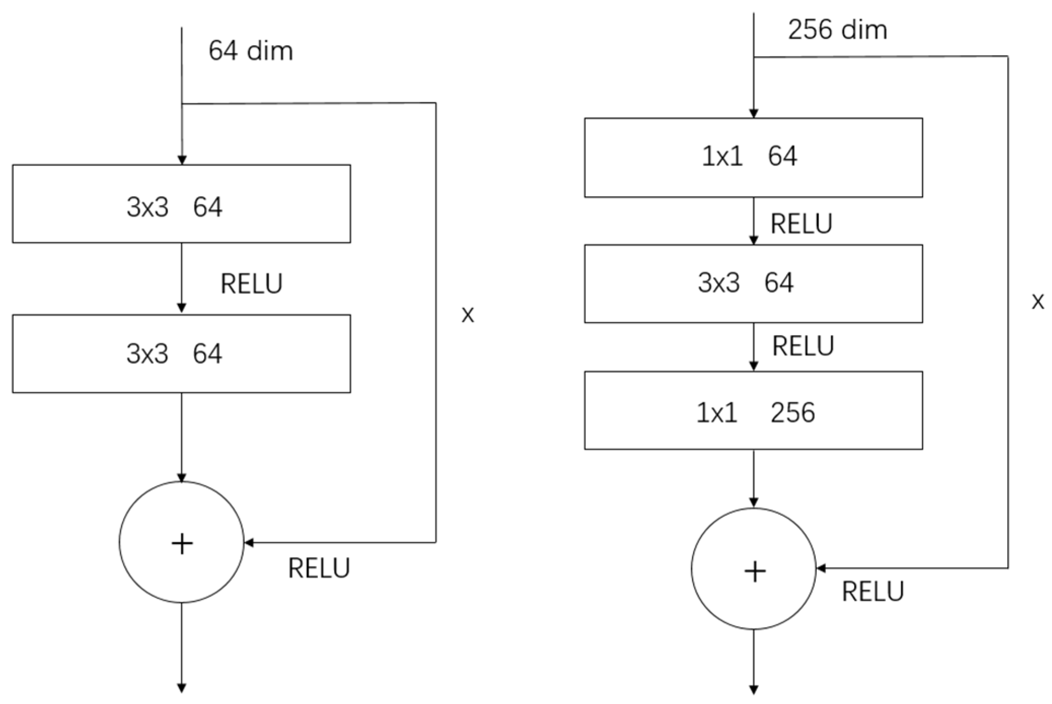
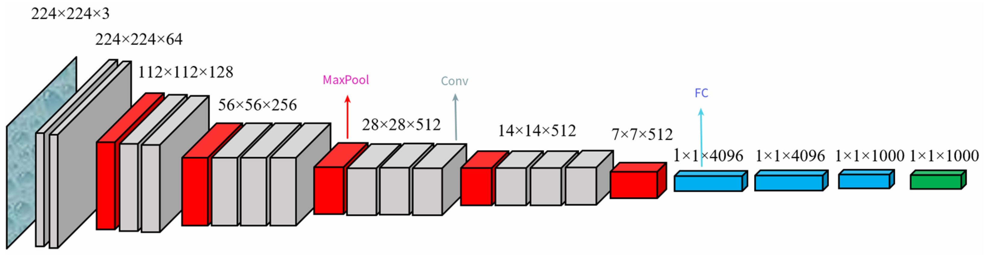
2.1. Backbone Network

The backbone network serves as a critical element in deep learning architectures, tasked with feature extraction from the input. These extracted features are pivotal for tasks like image classification and object detection. Comprising deep convolutional neural networks, backbone networks are adept at distilling semantically meaningful features from images. Prominent examples of such networks are ResNet, known for its residual learning framework, and VGGNet, recognized for its depth and architectural simplicity.

ResNet: ResNet (see Figure 1) is a type of deep learning model that processes residual functions related to the input through its weight layers. Developed in 2015 for image recognition, ResNet’s main innovation is the introduction of “residual blocks”. In conventional neural networks, each layer is designed to learn the direct mapping from input to output. Contrastingly, ResNet introduces a novel approach where layers are engineered to learn the residual mapping. This means that instead of learning the outright transformation from input to output, layers in ResNet focus on understanding the discrepancy, or residual, between the two. This design allows ResNet to train very deep network structures. With this approach, problems of vanishing gradients or exploding gradients do not worsen with the increase in network depth, which is a common issue when training deep neural networks. Another advantage of ResNet is that its residual structure does not lead to an increase in training error, even with more layers added. This means that network performance can be improved by adding more layers without increasing complexity.

VGGNet (see Figure 2) is distinguished by its architectural depth, with variants like VGG16 and VGG19 incorporating 16 and 19 hidden layers, respectively. These layers consist predominantly of convolutional and fully connected layers. A defining feature of VGGNet is the uniform use of convolutional kernels across all convolutional layers, streamlining the network’s structure for ease of comprehension. VGGNet’s primary strength lies in its robust performance, demonstrating proficiency in a range of computer vision applications, including image classification and object detection. However, its extensive parameter count necessitates significant computational power and memory allocation.

The selection of a backbone network is typically influenced by the task’s intricacy and the characteristics of the input image. Throughout the training phase, fine-tuning the backbone network’s parameters is a common practice to tailor it to the specific requirements of the task at hand. This customization process enhances the network’s ability to extract relevant features and improve performance on the designated task.

2.2. U-Net Network

U-Net is a specialized type of deep convolutional neural network designed for biomedical image segmentation, introduced by Ronneberger et al. [38] (see Figure 3).

U-Net, originally conceived for biomedical image segmentation, has gained prominence across a spectrum of semantic segmentation challenges due to its efficacy. At its heart lies a balanced encoder–decoder structure. The encoder component methodically distills features from the input through a series of convolutional and pooling layers, condensing them into a dense, low-dimensional representation. Subsequently, the decoder reverses this process, expanding the features to their initial dimensions via upsampling and convolutional layers and assigning a classification to each pixel. This symmetrical structure helps U-Net more effectively preserve spatial information in image segmentation, significantly improving segmentation accuracy.

Another notable feature of the network is the skip connections, which directly connect the corresponding layers of the encoder and decoder, promoting effective feature reconstruction and more precise segmentation. U-Net’s architecture is designed to compensate for the loss of feature maps during the encoder’s downsampling stages. By connecting these maps to the decoder’s layers in the upsampling phase, the network leverages comprehensive contextual details. This connection, known as ‘skip connections’, ensures that the decoder has access to both high-level and low-level features, facilitating precise segmentation. The ingenuity of U-Net’s design, particularly these skip connections, contributes significantly to its superior performance across diverse semantic segmentation applications.

2.3. Network Improvements Based on Attention Mechanisms

The attention mechanism in machine learning, drawing inspiration from the human visual attention system, selectively concentrates on pertinent regions within a scene. This mechanism, modeled after human visual and cognitive processes, seeks to direct the model’s focus toward the most salient information during data analysis. The advent of attention mechanisms has empowered neural networks to independently identify and prioritize crucial data elements, thereby markedly enhancing the efficiency and generalization capabilities of the model’s computational performance.

The fundamental principle of the attention mechanism lies in its ability to ascertain a distribution of weights, which it subsequently applies to the data attributes, thereby enhancing the model’s focus on significant features. These weights can be fully retained, known as soft attention, or partially retained, known as hard attention, which is based on a specific sampling strategy to select a subset of features. There are various forms of attention mechanisms, such as self-attention, spatial attention, and temporal attention. These mechanisms allow the model to assign different levels of importance to different parts of the input data, enabling it to focus on the most relevant information when processing each data element, thus achieving more precise data processing. The application of this method has made the attention mechanism excel in various complex tasks.

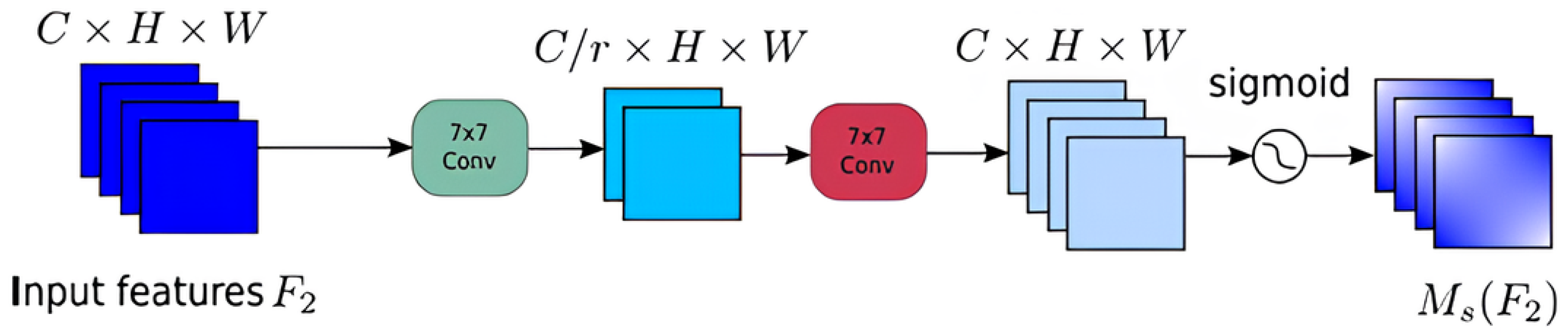
2.3.1. Spatial Attention Module

The spatial attention mechanism [39], prevalent in deep learning architectures, enables the model to prioritize critical spatial details within the input data. It operates by computing attention weights for distinct spatial locales, which are then allocated to the respective features. Consequently, the model intensifies its focus on pivotal locations during feature processing at each spatial coordinate. Specifically, the spatial attention mechanism is usually illustrated as shown in Figure 4.

The computation of attention weights commences with the model determining these weights for every spatial point within the input features, typically through a diminutive neural network such as a convolutional neural network. Subsequently, the model assigns the ascertained attention weights to each spatial position of the input features. In the concluding phase, the model amalgamates the weighted features to derive the ultimate output features. The spatial attention mechanism is frequently incorporated in diverse neural network models, enhancing their efficacy in functions including classification, detection, and segmentation.

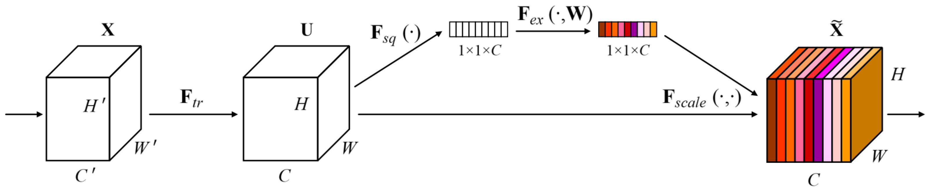
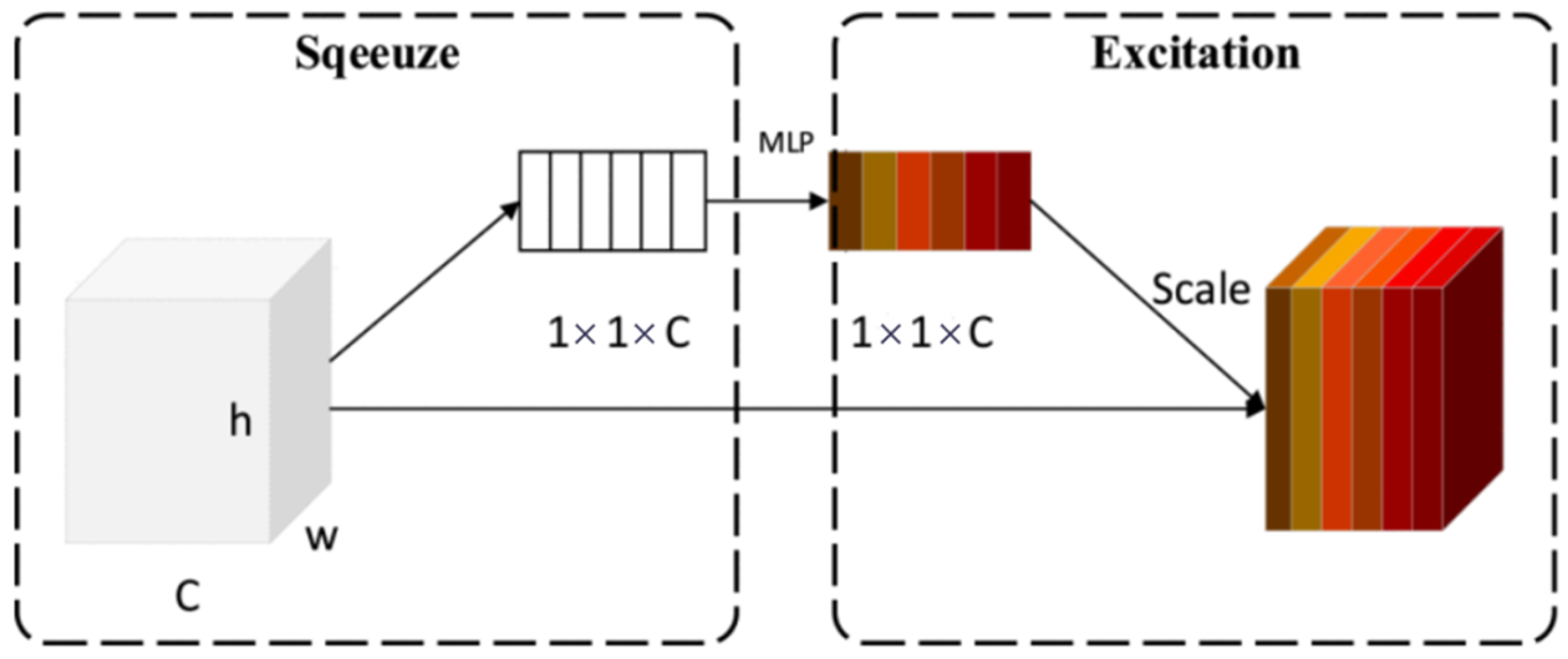
2.3.2. SE Attention Module

The SeNet attention mechanism [40] is part of the channel attention mechanism. This mechanism focuses on the interconnections between channels, improving model performance by learning the weights of different channels. SeNet consists of three operations: squeeze, excitation, and scale. The network structure is illustrated in Figure 5.

Squeeze operation: In layman’s terms, the squeeze operation transforms the global spatial features of the channels into a single global feature. During convolutional transformations across various channels, to better utilize contextual information and enhance the inter-channel correlation, global average pooling is used to compress the feature map. Specifically, this means reducing the dimensionality of the feature map while retaining only the channel information of the feature map.

Excitation operation: The excitation operation gathers information during the compression operation to capture channel dependencies. This method uses two fully connected layers to transform the feature map channels. The feature map channels are first reduced in dimensionality and then activated nonlinearly through an activation function; afterwards, the feature map is upsampled, and the output values are limited through a sigmoid function. The objective of this procedure is to recalibrate the feature set, streamline the model’s parameter complexity, and bolster its capacity for generalization.

Scale operation: This operation is for reweighting, which means reapplying all the attention weights to the features of each channel and multiplying by the feature weights to obtain the final output.

After these operations, SeNet can more effectively leverage the inter-channel correlations to enhance the model’s performance.

The Squeeze-and-Excitation SE module’s computational process unfolds in distinct phases:

Global Average Pooling: Initiated by applying global average pooling to the input feature map x, it produces a channel descriptor y. This descriptor quantifies the average activation per channel within the input feature map, formalized by the equation:

$$y=F_{avg}\left(x\right)={\displaystyle \frac{1}{H\times W}}\sum _{i=1}^H\sum _{j=1}^{W}x(i,j)$$

(1)

In this formula, H and W represent the height and width of the input feature map, respectively.

Fully Connected Layer: The channel descriptor y is then relayed through a fully connected layer, which consists of two sequential linear layers with an intervening ReLU activation function, to compute a channel weight vector. This is encapsulated by the equation:

$$fc\_out=W_2\cdot \mathrm{ReLU}(W_1\cdot y)$$

(2)

Here, $W_1$ and $W_2$ are the weights of the fully connected layers.

Sigmoid Activation: Finally, a sigmoid function is applied to constrain the channel weights between 0 and 1.

$$z=\sigma (fc\_out)={\displaystyle \frac{1}{1+e^{-fc\_out}}}$$

(3)

Thus, we obtain the attention weights for each channel, which can be considered as the importance of that channel. In subsequent computations, these weights will be used to adjust the response of each channel, allowing the model to focus on more important channels.

2.3.3. Channel Attention Module

The channel attention mechanism dynamically modulates feature map weights within the channel domain, selectively emphasizing salient features [41]. This mechanism is efficiently integrated with dense blocks and transition layers to enhance feature representation without significantly increasing the parameter count. The architecture of the channel attention network is compact and designed to prevent overfitting.

The transition layer, comprising a 1 × 1 convolutional layer followed by average pooling with a stride of two, effectively reduces feature map dimensions. This integration of the channel attention module with the transition layer, termed adaptive downsampling, is depicted in Figure 6. The mechanism operates in a two-stage process: “squeeze” and “excitation”.

During the squeeze stage, input features are condensed into a one-dimensional vector corresponding to the number of feature channels. This compression is achieved through global average pooling across spatial domains, yielding a vector representing channel intensities. Subsequently, in the excitation stage, inter-channel dependencies are modeled via a gating mechanism involving two nonlinear, fully connected layers. By modulating channel weights, the channel attention module adaptively prioritizes certain features, thereby enhancing model performance with a minimal parameter increase, unlike conventional feature-map-focused attention models.

The channel attention class’s main role is to calculate the attention weights, signifying the significance of each channel. This calculation involves several steps:

Global average pooling and Global Max Pooling operations are applied to the input feature map, denoted as x, yielding two distinct channel descriptors: avg_out and max_out. These descriptors, respectively, encapsulate the average and peak responses across the channels within the input feature map.

$$avg\_out=F_{avg}\left(x\right)={\displaystyle \frac{1}{H\times W}}\sum _{i=1}^H\sum _{j=1}^{W}x(i,j)$$

(4)

$$max\_out=F_{max}\left(x\right)=\stackrel{H,W}{\underset{i=1,j=1}{max}}x(i,j)$$

(5)

In the fully connected layer, the channel descriptors avg_out and max_out undergo processing through the fully connected layer. This layer consists of two convolutional layers coupled with a ReLU activation function, culminating in the generation of two channel weight vectors.

$$fc\_out=W_2\cdot \mathrm{ReLU}(W_1\cdot x)$$

(6)

$W_1$ and $W_2$ are the weights of the fully connected layer, and the dot ⋅ represents the convolution operation.

Weighted Sum: The descriptors avg_out and max_out are combined through a weighted sum to derive the final channel weights.

$$out=fc(avg\_out)+fc(max\_out)$$

(7)

Subsequently, a sigmoid activation function constrains these weights within the range [0, 1].

$$y=\sigma \left(out\right)={\displaystyle \frac{1}{1+e^{-out}}}$$

(8)

At this point, the attention weights for each channel are obtained, which can be regarded as the importance of that channel. In the subsequent computational steps, these derived weights are applied to modulate each channel’s response. This modulation enables the model to prioritize channels of greater importance.

3. Dataset and Results

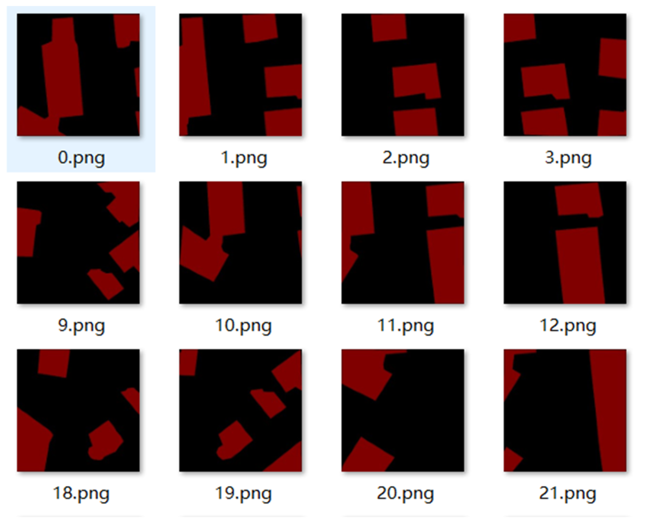
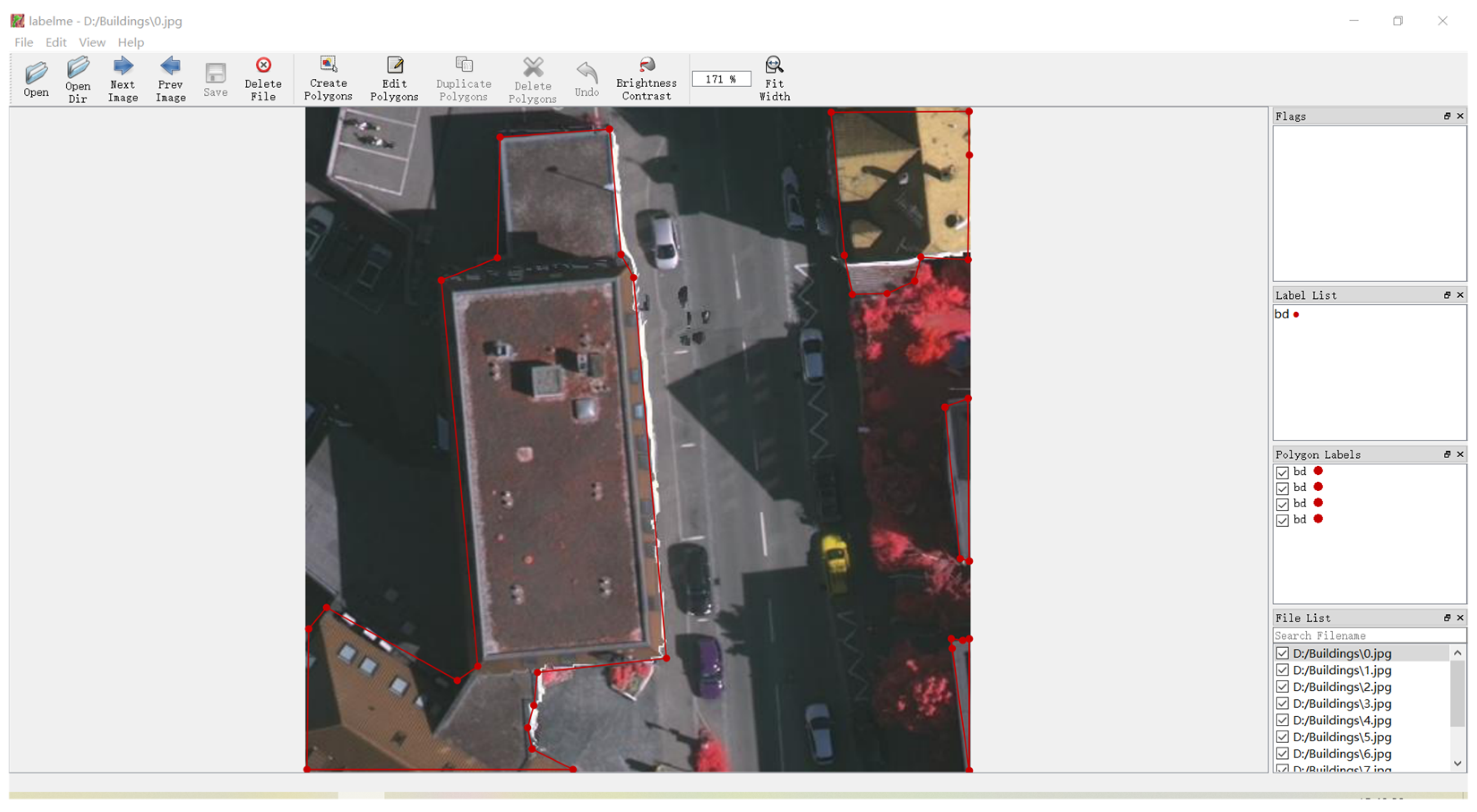
3.1. Datasets and Preprocessing

In the preparation phase of the experiment, 100 small datasets with semantic labels were labeled for feasibility experiments, including backgrounds and buildings, as shown in Figure 7. Labelme 4.5.6 was used to label the collected images, which contain two types of labels, namely background and building, indicating the background and building. The production methodology during the labeling process is illustrated in Figure 8.

For deep learning, having a small dataset and performing only binary classification can lead to artificially high accuracy. In this instance, the dataset underwent division into training, validation, and test subsets, adhering to an 8:1:1 ratio. After training the model on this limited dataset, the accuracy approached 100%, but this high accuracy is likely due to the small dataset and binary classification.

To further investigate model feasibility, we used a small manually labeled dataset. However, for more comprehensive experiments, we decided to use a larger dataset with more diverse classes and finer semantic segmentation labels.

The dataset used in this study is the publicly available Vaihingen dataset. The dataset encompasses 33 patches of varying dimensions, each segmented from an extensive true orthophoto (TOP) mosaic. The spatial resolution for both the TOP imagery and the digital surface models (DSMs) stands at 9 cm. The remote sensing images, formatted as 8-bit TIFF files, comprise three spectral bands: near-infrared, red, and green. Within this dataset, there are variously shaped large and small buildings, and the semantic labels are well-defined, making it suitable for model training.

The dataset consists of 33 distinct patches, each varying in size and meticulously extracted from a comprehensive true orthophoto (TOP) mosaic. The TOP imagery and digital surface models (DSMs) boast a fine spatial resolution of 9 cm. Comprising three spectral bands—near-infrared, red, and green—the remote sensing images are provided as 8-bit TIFF files.

The Vaihingen dataset is annotated with six distinct semantic labels: opaque water bodies, vehicles, trees, low vegetation, buildings, and background. Since the original images are large, they are cropped into 3300 smaller images (see Figure 9). Each label within the Vaihingen dataset is presented in an RGB format with a resolution of 512 × 512 pixels. For the purposes of model training and evaluation, the dataset has been partitioned into training, validation, and test sets following an 8:1:1 ratio.

However, at this time, the dataset cannot be directly used for training, and the label needs to be converted to gray level. Deep learning models in PyTorch 2.3.0 typically expect labels to be single-channel, where the value of each pixel corresponds to the class number. This is because during training, the model needs to compare the labels with the predicted results, calculate the losses, and perform gradient updates. If the label possesses multiple channels, it requires conversion to a single channel format to align with the model’s output. The dataset’s semantic information is detailed in

Table 1. Semantic information and channel values.

Semantic Information	ID	RGB Channel Value
Background	0	(RGB: 255, 0, 0)
Car	1	(RGB: 255, 255, 0)
Tree	2	(RGB: 0, 255, 0)
Low vegetation	3	(RGB: 0, 255, 255)
Building	4	(RGB: 0, 0, 255)
Impervious surface	5	(RGB: 255, 255, 255)

, while the post-conversion effect is depicted in Figure 10.

3.2. Experimental Environment and Evaluation Index

3.2.1. Experimental Environment

In this study, all algorithms were executed within the PyTorch framework. The experimental operating environment is outlined in

Table 2. The operating environment of the experiment.

Disposition	Model
CPU model	Intel® Core™ i5-10400 CPU:Santa Clara, CA, USA
GPU version	NVIDIA GeForce RTX 2060: Santa Clara, CA, USA
Hard disk	Kingston SA2000M8500G (A2000 NVMe PCIe SSD):Fountain Valley, CA, USA
Main board	N9x0SD2
python	3.9
torch	2.3.0
CUDA	12.4

.

The training parameters are delineated in

Table 3. Model base parameter.

Argument	Value
batch size	4
epoch	20
Input size	512 × 512
Init_lr	0.0001
optimizer_type	adam
momentum	0.9
num_classes	6

, where Init_lr denotes the initial learning rate. The term optimizer_type refers to the chosen optimizer, while momentum pertains to the parameters utilized within the optimizer, primarily for the modification of the learning rate. The variable num_classes indicates the quantity of classifications for remote sensing images, encompassing categories like buildings, meadows, and others. Input_size specifies the dimensions of the input image, and epochs represents the aggregate number of training iterations for the model.

3.2.2. Model Evaluation Index

The evaluation metrics employed in this experiment encompass accuracy, pixel accuracy, mean pixel accuracy, and mean intersection over union (IoU). The computation of these metrics in image semantic segmentation unfolds in two phases: first, calculate the corresponding indicators. The IoU metric quantifies the overlap between the predicted and actual values. A prediction is deemed accurate if the overlap exceeds a predefined threshold. This approach categorizes predictions into four outcomes: true positive (TP), false positive (FP), true negative (TN), and false negative (FN). Typically, there is an inverse relationship between accuracy and recall; hence, the f_score is introduced as a comprehensive evaluation metric. The f_score harmonizes the effects of accuracy and recall, providing a more balanced assessment of a classifier’s performance. It is calculated as the harmonic mean of precision and recall.

$$\mathrm{f}\_\mathrm{s}\mathrm{c}\mathrm{o}\mathrm{r}\mathrm{e}=2\times {\displaystyle \frac{\mathrm{A}\mathrm{c}\mathrm{c}\mathrm{u}\mathrm{r}\mathrm{a}\mathrm{c}\mathrm{y}\times \mathrm{Recall}}{\mathrm{A}\mathrm{c}\mathrm{c}\mathrm{u}\mathrm{r}\mathrm{a}\mathrm{c}\mathrm{y}+\mathrm{Recall}}}$$

(9)

Among them, accuracy refers to the probability of correct detection among all detected targets, so its formula is shown as Equation (10):

$$\mathrm{A}\mathrm{c}\mathrm{c}\mathrm{u}\mathrm{r}\mathrm{a}\mathrm{c}\mathrm{y}={\displaystyle \frac{\mathrm{T}\mathrm{P}}{\mathrm{T}\mathrm{P}+\mathrm{F}\mathrm{P}}}$$

(10)

Recall refers to the probability of correct detection in all positive samples, so its formula is expressed as (11).

$$\mathrm{R}\mathrm{e}\mathrm{c}\mathrm{a}\mathrm{l}\mathrm{l}={\displaystyle \frac{\mathrm{T}\mathrm{P}}{\mathrm{T}\mathrm{P}+\mathrm{F}\mathrm{N}}}$$

(11)

Pixel Accuracy: This is the simplest metric, which is the percentage of the total pixels that are correctly labeled. Therefore, its formula expression is shown in Equation (12):

$$\mathrm{P}\mathrm{A}={\displaystyle \frac{\sum _{i=0}^k{p}_{ii}}{{\sum }_{i=0}^k\sum _{j=0}^k{p}_{ij}}}$$

(12)

Mean Pixel Accuracy: This is a simple improvement of PA, calculating the proportion of pixels that are correctly classified in each class and then finding the average of all classes. Its formula is shown in Equation (13):

$$\mathrm{M}\mathrm{P}\mathrm{A}={\displaystyle \frac{1}{k+1}}{\sum }_{i=0}^k{\displaystyle \frac{p_{ii}}{{\sum }_{j=0}^k{p}_{ij}}}$$

(13)

Mean Intersection over Union: This is a key index to evaluate the performance of semantic segmentation. It measures accuracy by calculating the proportion of the intersection and union between the predicted and true splits. In the case of semantic segmentation, this ratio can be morphed into the sum of intersection over true, false negative, and false positive (union). IoU is calculated on each class and then averaged. The expression of the formula is shown in Equation (14):

$$\mathrm{M}\mathrm{I}\mathrm{o}\mathrm{u}={\displaystyle \frac{1}{k+1}}{\sum }_{i=0}^k{\displaystyle \frac{p_{ii}}{{\sum }_{j=0}^k{p}_{ij}+{\sum }_{j=0}^k{p}_{ji}-p_{ii}}}$$

(14)

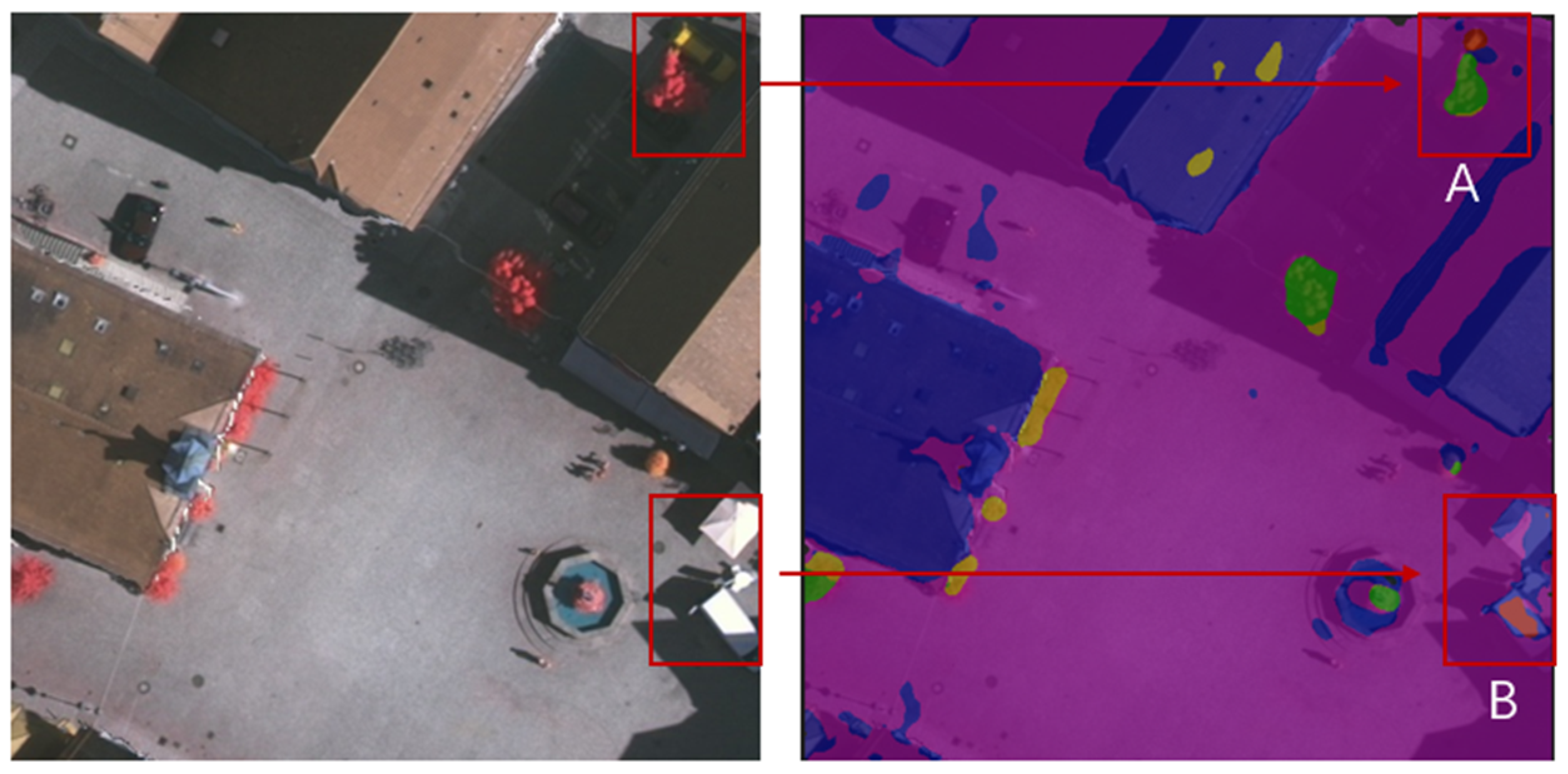
3.3. Experimental Results

3.3.1. Trunk Network Selection Comparative Experiment

The neural network undergoes training and testing utilizing the public dataset detailed in Section 3.1. Post-training, the temporal progression and experimental outcomes are depicted in Figure 11, where parts (a) and (b) correspond to the variations in f_score and total_loss for various backbone networks as a function of the epoch during the training phase. total_loss is the total loss value calculated by the model during the training process. If CE_Loss is selected, use Formula (15); if Focal_Loss is selected, use Formula (16).

Subsequently, the trained model is evaluated on the identical test set to assess the intersection ratio, average pixel accuracy, and accuracy across different models. The comparative results are presented in

Table 4. Average pixel accuracy and accuracy between different models.

Model	MPA	MIoU
Resnet50+Unet	53.59	42.95
Unet	71.85	59.44
Vgg+Unet	87.12	75.83

.

The conclusive data from the experiment indicate that the model’s accuracy stands at 90.12%, the average crossover ratio is 75.83%, and the average pixel accuracy is 87.12%, which is satisfactory under the condition of less training time. The accuracy rate of the Resnet50+Unet network was 74.44%, and that of MIoU was 42.95. The U-Net network surpasses the Resnet50+Unet in terms of accuracy, yet it falls short when compared to the Vgg+Unet. Figure 12 and Figure 13 depict the comparative predictive efficacy of the Resnet50+Unet and Vgg+Unet models, with the former demonstrating superior recognition of trees and cars in region A, as well as buildings in region B, relative to the latter’s performance in regions C and D. Therefore, Vgg is chosen as the backbone network and continues to be improved as the basic model.

3.3.2. An Improved Experiment Based on Vgg+Unet Network

In terms of basic network improvement, after comparing U-Net, Resnet50+Unet, and Vgg+Unet, Vgg as the backbone network achieved the best accuracy. To enhance the model’s detection accuracy, subsequent refinements to the architecture will be pursued, building upon the existing framework. This study incorporated three distinct attention mechanisms—spatial, SE, and channel—into the backbone network for individual evaluation. A comparative analysis of their detection impacts was conducted. The outcomes of these experimental comparisons are presented in

Table 5. Average pixel accuracy and accuracy between different models (CE_loss).

Attention Mechanism	MPA	MIoU	Accuracy
Vgg+Unet	87.12	75.83	90.12
Spatial	87.77	79.35	90.28
SE	88.66	79.23	90.58
Channel	87.87	80.65	91.26

.

Initially, the basic model employed CE_loss (the calculation method is shown in Formula (15)), a standard loss function in deep learning. To investigate potential performance enhancements, the model’s loss function was transitioned to Focal_loss (the calculation method is shown in Formula (16)). This modification introduces an adjustment factor to CE_loss, directing the model’s focus toward challenging-to-classify samples and potentially boosting recognition accuracy for minority classes. Subsequent to this alteration, the detection accuracies of the three attention mechanisms were re-evaluated, with findings detailed in

Table 6. Average pixel accuracy and accuracy between different models (Focal_loss).

Attention Mechanism	MPA	MIoU	Accuracy
Vgg+Unet	87.12	75.83	90.12
Spatial	86.72	78.44	89.49
SE	87.36	78.19	89.95
Channel	87.57	79.40	90.46

.

$$H(y,\widehat{y})=-\sum _i{y}_i\mathrm{l}\mathrm{o}\mathrm{g}\left({\widehat{y}}_i\right)$$

(15)

$$FL\left(p_t\right)=-{\alpha }_t(1-p_t{)}^{\gamma }\mathrm{l}\mathrm{o}\mathrm{g}(p_t)$$

(16)

The experimental findings indicate that altering the loss function to Focal_Loss did not yield the anticipated improvement. Instead, there was a marginal reduction in accuracy compared to when CE_loss was utilized. This can be attributed to Focal_Loss’s design, which emphasizes addressing class imbalances within datasets. As the public dataset used in this study is relatively balanced, the model’s accuracy experienced a slight decline with the implementation of Focal_Loss.

By comparing the addition of attention mechanisms under different loss functions, we can see that although the addition of attention mechanisms will make the training time longer, the training time will increase by about one-third compared with the basic model. But accuracy could be improved. The integration of spatial and SE attention mechanisms has been observed to modestly enhance accuracy, with the spatial attention mechanism contributing a 0.16% increase and the SE attention mechanism providing a 0.46% boost. In contrast, the channel attention mechanism significantly outperforms the aforementioned mechanisms by elevating accuracy by 1.14% when compared to models without any attention mechanisms. Additionally, both MPA and MioU metrics exhibit notable improvements. Consequently, CE_loss is retained as the loss function, and ablation studies employing the refined method are conducted, with the outcomes detailed in

Table 7. Improvement of basic network model and results of ablation experiment.

Network	Vgg	Channel	CE_Loss	MPA	MIoU	Accuracy
				71.85	59.44	79.84
	√			87.12	75.83	90.12
U-Net	√	√		87.57	79.40	90.46
	√		√	72.38	72.38	89.41
	√	√	√	87.87	80.65	91.26

.

According to the comparison results, the final improved Vgg+Unet+Channel network model has the best segmentation accuracy under the CE_loss function. The Vgg+Unet network has been enhanced by integrating a channel attention mechanism, resulting in the upgraded Vgg+Unet+Channel network model. This advancement incorporates the refined attention mechanism into the neural network’s architecture. The detection effect is shown in Figure 14, Figure 15 and Figure 16. After the prediction results, the statistics of pixels in each category can be carried out, as shown in

Table 8. The proportion of each semantic in Figure 15.

Semantic Information	Number of Pixels	Percentage of Surface
Impervious surface	13,704	0.20%
Car	21,243	0.32%
Tree	1,380,016	20.54%
Low vegetation	1,786,765	26.60%
Building	1,601,524	23.84%
Background	1,915,024	28.50%

and

Table 9. The proportion of each semantic in Figure 16.

Semantic Information	Number of Pixels	Percentage of Surface
Impervious surface	6927	0.14%
Car	37,879	0.79%
Tree	174,257	3.61%
Low vegetation	176,063	3.65%
Building	3,433,466	71.16%
Background	996,467	20.65%

, in order to find out the area occupied by different semantic information.

4. Conclusions

The ongoing advancements in remote sensing technology enable the acquisition of increasingly high-quality images. These images facilitate a precise understanding of urban expansion. This paper delves into the neural network-based image semantic segmentation method, focusing on the diverse plot information within remote sensing imagery as the subject of investigation.

Initially, the labelme tool facilitated data annotation, segregating it into two distinct categories to assess the model’s viability. The requisite torch operating environment was established, various network models underwent training, and analytical scrutiny of the experimental outcomes led to the selection of the most efficacious neural network model as the foundational network. To augment accuracy, the introduction of an attention mechanism was deemed necessary to enhance the evaluation metric. Consequently, spatial, SE, and channel attention mechanisms were integrated into the backbone network, and a comparative analysis was conducted to determine the optimal loss function. Through experimental comparison, it was found that CE_loss had a better performance than Focal_loss, because the classification imbalance in the dataset was not significant. Finally, CE_loss was selected as the loss function. After the analysis and comparison of the experimental results, spatial and SE attention mechanisms slightly improved the segmentation accuracy, but the channel attention mechanism had a more significant improvement, and the accuracy was increased by 1.14% compared with the basic network. The training time of the three groups was similar, but the training time was also about one-third longer than when the attention mechanism was not added. Finally, according to the experimental comparison, the channel attention mechanism was selected as the final model. The final experimental results show that the proposed Vgg+Unet+Channel network model had a good effect on small sample image segmentation.

References

1. Bhargavi, K.; Jyothi, S. A survey on threshold based segmentation technique in image processing. Int. J. Innov. Res. Dev. 2014, 3, 234–239. [Google Scholar]
2. Cai, H.; Yang, Z.; Cao, X.; Xia, W.; Xu, X. A new iterative triclass thresholding technique in image segmentation. IEEE Trans. Image Process. 2014, 23, 1038–1046. [Google Scholar] [CrossRef] [PubMed]
3. Bieniek, A.; Moga, A. An efficient watershed algorithm based on connected components. Pattern Recognit. 2000, 33, 907–916. [Google Scholar] [CrossRef]
4. Chien, S.Y.; Huang, Y.W.; Chen, L.G. Predictive watershed: A fast watershed algorithm for video segmentation. IEEE Trans. Circuits Syst. Video Technol. 2003, 13, 453–461. [Google Scholar] [CrossRef]
5. Zhou, S.; Wang, J.; Zhang, S.; Liang, Y.; Gong, Y. Active contour model based on local and global intensity information for medical image segmentation. Neurocomputing 2016, 186, 107–118. [Google Scholar] [CrossRef]
6. Wang, L.; Chang, Y.; Wang, H.; Wu, Z.; Pu, J.; Yang, X. An active contour model based on local fitted images for image segmentation. Inf. Sci. 2017, 418, 61–73. [Google Scholar] [CrossRef] [PubMed]
7. Xu, Y.; Wu, L.; Xie, Z.; Chen, Z. Building extraction in very high resolution remote sensing imagery using deep learning and guided filters. Remote Sens. 2018, 10, 144. [Google Scholar] [CrossRef]
8. Li, R.; Liu, W.; Yang, L.; Sun, S.; Hu, W.; Zhang, F.; Li, W. DeepUNet: A deep fully convolutional network for pixel-level sea-land segmentation. IEEE J. Sel. Top. Appl. Earth Obs. Remote Sens. 2018, 11, 3954–3962. [Google Scholar] [CrossRef]
9. Yi, Y.; Zhang, Z.; Zhang, W.; Zhang, C.; Li, W.; Zhao, T. Semantic segmentation of urban buildings from VHR remote sensing imagery using a deep convolutional neural network. Remote Sens. 2019, 11, 1774. [Google Scholar] [CrossRef]
10. Ding, L.; Tang, H.; Bruzzone, L. LANet: Local attention embedding to improve the semantic segmentation of remote sensing images. IEEE Trans. Geosci. Remote Sens. 2020, 59, 426–435. [Google Scholar] [CrossRef]
11. Shao, Z.; Zhou, W.; Deng, X.; Zhang, M.; Cheng, Q. Multilabel remote sensing image retrieval based on fully convolutional network. IEEE J. Sel. Top. Appl. Earth Obs. Remote Sens. 2020, 13, 318–328. [Google Scholar] [CrossRef]
12. Li, H.; Qiu, K.; Chen, L.; Mei, X.; Hong, L.; Tao, C. SCAttNet: Semantic segmentation network with spatial and channel attention mechanism for high-resolution remote sensing images. IEEE Geosci. Remote Sens. Lett. 2020, 18, 905–909. [Google Scholar] [CrossRef]
13. Xu, Z.; Zhang, W.; Zhang, T.; Li, J. HRCNet: High-resolution context extraction network for semantic segmentation of remote sensing images. Remote Sens. 2020, 13, 71. [Google Scholar] [CrossRef]
14. Li, R.; Zheng, S.; Zhang, C.; Duan, C.; Su, J.; Wang, L.; Atkinson, P.M. Multiattention network for semantic segmentation of fine-resolution remote sensing images. IEEE Trans. Geosci. Remote Sens. 2021, 60, 1–13. [Google Scholar] [CrossRef]
15. Gao, L.; Liu, H.; Yang, M.; Chen, L.; Wan, Y.; Xiao, Z.; Qian, Y. STransFuse: Fusing swin transformer and convolutional neural network for remote sensing image semantic segmentation. IEEE J. Sel. Top. Appl. Earth Obs. Remote Sens. 2021, 14, 10990–11003. [Google Scholar] [CrossRef]
16. Li, H.; Li, Y.; Zhang, G.; Liu, R.; Huang, H.; Zhu, Q.; Tao, C. Global and local contrastive self-supervised learning for semantic segmentation of HR remote sensing images. IEEE Trans. Geosci. Remote Sens. 2022, 60, 1–14. [Google Scholar] [CrossRef]
17. He, X.; Zhou, Y.; Zhao, J.; Zhang, D.; Yao, R.; Xue, Y. Swin transformer embedding UNet for remote sensing image semantic segmentation. IEEE Trans. Geosci. Remote Sens. 2022, 60, 1–15. [Google Scholar] [CrossRef]
18. Xu, R.; Wang, C.; Zhang, J.; Xu, S.; Meng, W.; Zhang, X. Rssformer: Foreground saliency enhancement for remote sensing land-cover segmentation. IEEE Trans. Image Process. 2023, 32, 1052–1064. [Google Scholar] [CrossRef]
19. Li, Y.; Chen, W.; Huang, X.; Gao, Z.; Li, S.; He, T.; Zhang, Y. MFVNet: A deep adaptive fusion network with multiple field-of-views for remote sensing image semantic segmentation. Sci. China Inf. Sci. 2023, 66, 140305. [Google Scholar] [CrossRef]
20. Ma, Z.; Xia, M.; Lin, H.; Qian, M.; Zhang, Y. FENet: Feature enhancement network for land cover classification. Int. J. Remote Sens. 2023, 44, 1702–1725. [Google Scholar] [CrossRef]
21. Li, X.; Xu, F.; Liu, F.; Lyu, X.; Tong, Y.; Xu, Z.; Zhou, J. A synergistical attention model for semantic segmentation of remote sensing images. IEEE Trans. Geosci. Remote Sens. 2023, 61, 1–16. [Google Scholar] [CrossRef]
22. Chen, J.; Xia, M.; Wang, D.; Lin, H. Double branch parallel network for segmentation of buildings and waters in remote sensing images. Remote Sens. 2023, 15, 1536. [Google Scholar] [CrossRef]
23. Song, P.; Li, J.; An, Z.; Fan, H.; Fan, L. CTMFNet: CNN and transformer multiscale fusion network of remote sensing urban scene imagery. IEEE Trans. Geosci. Remote Sens. 2022, 61, 1–14. [Google Scholar] [CrossRef]
24. Fu, Y.; Zhang, X.; Wang, M. DSHNet: A Semantic Segmentation Model of Remote Sensing Images based on Dual Stream Hybrid Network. IEEE J. Sel. Top. Appl. Earth Obs. Remote Sens. 2024, 17, 4164–4175. [Google Scholar] [CrossRef]
25. Pang, S.; Shi, Y.; Hu, H.; Ye, L.; Chen, J. PTRSegNet: A Patch-to-Region Bottom-Up Pyramid Framework for the Semantic Segmentation of Large-Format Remote Sensing Images. IEEE J. Sel. Top. Appl. Earth Obs. Remote Sens. 2024, 17, 3664–3673. [Google Scholar] [CrossRef]
26. Wang, M.; She, A.; Chang, H.; Cheng, F.; Yang, H. A deep inverse convolutional neural network-based semantic classification method for land cover remote sensing images. Sci. Rep. 2024, 14, 7313. [Google Scholar] [CrossRef]
27. Li, H.; Li, L.; Zhao, L.; Liu, F. ResU-Former: Advancing Remote Sensing Image Segmentation with Swin Residual Transformer for Precise Global–Local Feature Recognition and Visual–Semantic Space Learning. Electronics 2024, 13, 436. [Google Scholar] [CrossRef]
28. Xin, Y.; Fan, Z.; Qi, X.; Geng, Y.; Li, X. Enhancing Semi-Supervised Semantic Segmentation of Remote Sensing Images via Feature Perturbation-Based Consistency Regularization Methods. Sensors 2024, 24, 730. [Google Scholar] [CrossRef]
29. Yang, Y.; Wang, Y.; Dong, J.; Yu, B. A Knowledge Distillation-based Ground Feature Classification Network with Multiscale Feature Fusion in Remote Sensing Images. IEEE J. Sel. Top. Appl. Earth Obs. Remote Sens. 2023, 17, 2347–2359. [Google Scholar] [CrossRef]
30. Xie, J.; Pan, B.; Xu, X.; Shi, Z. MiSSNet: Memory-inspired Semantic Segmentation Augmentation Network for Class-Incremental Learning in Remote Sensing Images. IEEE Trans. Geosci. Remote Sens. 2024, 62, 5607913. [Google Scholar] [CrossRef]
31. Zhang, L.; Tan, Z.; Zhang, G.; Zhang, W.; Li, Z. Learn more and learn useful: Truncation Compensation Network for Semantic Segmentation of High-Resolution Remote Sensing Images. IEEE Trans. Geosci. Remote Sens. 2024, 62, 4403814. [Google Scholar]
32. Zhao, W.; Cao, J.; Dong, X. Multilateral Semantic with Dual Relation Network for Remote Sensing Images Segmentation. IEEE J. Sel. Top. Appl. Earth Obs. Remote Sens. 2023, 17, 506–518. [Google Scholar] [CrossRef]
33. Liu, J.; Hua, W.; Zhang, W.; Liu, F.; Xiao, L. Stair Fusion Network with Context Refined Attention for Remote Sensing Image Semantic Segmentation. IEEE Trans. Geosci. Remote Sens. 2024, 62, 4701517. [Google Scholar] [CrossRef]
34. Bai, Q.; Luo, X.; Wang, Y.; Wei, T. DHRNet: A Dual-branch Hybrid Reinforcement Network for Semantic Segmentation of Remote Sensing Images. IEEE J. Sel. Top. Appl. Earth Obs. Remote Sens. 2024, 17, 4176–4193. [Google Scholar] [CrossRef]
35. Kumar, S.; Kumar, A.; Lee, D.G. RSSGLT: Remote Sensing Image Segmentation Network based on Global-Local Transformer. IEEE Geosci. Remote Sens. Lett. 2023, 21, 8000305. [Google Scholar] [CrossRef]
36. Wang, W.; Ran, L.; Yin, H.; Sun, M.; Zhang, X.; Zhang, Y. Hierarchical Shared Architecture Search for Real-time Semantic Segmentation of Remote Sensing Images. IEEE Trans. Geosci. Remote Sens. 2024, 62, 1–13. [Google Scholar] [CrossRef]
37. Ullah, A.; Elahi, H.; Sun, Z.Y.; Khatoon, A.; Ahmad, I. Comparative Analysis of AlexNet, ResNet18 and SqueezeNet with Diverse Modification and Arduous Implementation. Arab. J. Sci. Eng. 2022, 47, 2397–2417. [Google Scholar] [CrossRef]
38. Ronneberger, O.; Fischer, P.; Brox, T. U-net: Convolutional networks for biomedical image segmentation. In Medical Image Computing and Computer-Assisted Intervention, Proceedings of the MICCAI 2015: 18th International Conference, Munich, Germany, 5–9 October 2015; Proceedings, Part III 18; Springer International Publishing: Berlin/Heidelberg, Germany, 2015; pp. 234–241. [Google Scholar]
39. Chen, L.; Zhang, H.; Xiao, J.; Nie, L.; Shao, J.; Liu, W.; Chua, T.S. SCA-CNN: Spatial and Channel-Wise Attention in Convolutional Networks for Image Captioning. In Proceedings of the 2017 IEEE Conference on Computer Vision and Pattern Recognition (CVPR), Honolulu, HI, USA, 21–26 July 2017; pp. 6298–6306. [Google Scholar] [CrossRef]
40. Hu, J.; Shen, L.; Sun, G. Squeeze-and-excitation networks. In Proceedings of the IEEE Conference on Computer Vision and Pattern Recognition, Salt Lake City, UT, USA, 18–23 June 2018; pp. 7132–7141. [Google Scholar]
41. Guo, M.H.; Xu, T.X.; Liu, J.J.; Liu, Z.N.; Jiang, P.T.; Mu, T.J.; Zhang, S.H.; Martin, R.R.; Cheng, M.M.; Hu, S.M. Attention mechanisms in computer vision: A survey. Comput. Vis. Media 2022, 8, 331–368. [Google Scholar] [CrossRef]
Figure 1. Network structure of ResNet.
Applsci 14 07499 g001
Figure 2. Network structure of Vgg.
Applsci 14 07499 g002
Figure 3. Network structure of U-Net [38].
Applsci 14 07499 g003
Figure 4. Spatial attention mechanism.
Applsci 14 07499 g004
Figure 5. SeNet module structure.
Applsci 14 07499 g005
Figure 6. Channel module structure.
Applsci 14 07499 g006
Figure 7. Dataset label.
Applsci 14 07499 g007
Figure 8. Labelme data annotation.
Applsci 14 07499 g008
Figure 9. Cropped dataset.
Applsci 14 07499 g009
Figure 10. Converted to grayscale after the label.
Applsci 14 07499 g010
Figure 11. f_score and total_loss change with epoch and training time.
Applsci 14 07499 g011
Figure 12. Prediction effect of Resnet50+Unet model, Area A contains trees and cars; Area B contains buildings and cars.
Applsci 14 07499 g012
Figure 13. Prediction effect of Vgg+Unet model, Area C contains trees and cars; Area D contains buildings and cars.
Applsci 14 07499 g013
Figure 14. Comparison of different models with a loss function of CE_loss, (a) original figure; (b) Channel; (c) SE; (d) Spatial; (e) VGG.
Applsci 14 07499 g014
Figure 15. The model semantic information prediction results 1.
Applsci 14 07499 g015
Figure 16. The model semantic information prediction results 2.
Applsci 14 07499 g016