1. Introduction
In 1972, Nasir Ahmed proposed the discrete cosine transform for the first time [
1]. It is well known under the abbreviation DCT. DCT plays a crucial role in the digital world, being used in data compression and coding for digital images (DCT is the base of the JPEG 1 standard—ISO/IEC 10918 [
2]) [
3,
4], digital audio (used in modern audio coding standards like Dolby Digital, WMA, MP3, HDC, MPEG-H 3D Audio or AAC) [
5], speech coding (such as AAC-LD, Siren, G.722.1, G.729.1 and Opus) [
6,
7], digital radio (such as AAC+ and DAB+) [
8], digital video (such as H.261, H.263, H.264 (AVC or MPEG-4), H.265 (HEVC or MPEG-H Part 2) and H.266) [
9,
10], or digital television (in video coding standards for SDTV, HDTV, and VOD) [
9,
10].
In 2017, internet video traffic was 73% of all worldwide consumer traffic. Right now, this percentage is more than 80% [
11]. The pandemic outbreak reinforced and supported this growth and the necessity of users to use video material. Moreover, a gradual transition from the SD (standard-definition) video format to the HD (high-definition) video format is observed, moving now towards the UHD (ultra-high-definition) video format [
9,
10].
From all of these, we have observed that DCT and its variants are extensively used in all modern audio, image, and video compression standards [
4,
7]. There are several types of DCT transforms, but the most known ones are DCT II, DCT III, and DCT IV. The DCT IV and DST IV were first introduced by Jain [
12] and have some important applications, such as spectral analysis, audio and image coding, and signal processing [
13,
14,
15].
Both DCT IV and DST IV are computationally intensive, and, for real-time applications, fast software [
16,
17,
18,
19] and even more parallel software implementations or hardware implementations [
20,
21] are required. In order to obtain efficient parallel software implementations, some efficient restructuring solutions to put in evidence parallel structures with reduced arithmetic complexity are required. But, until now, there have only been a few parallel software implementations for DCT IV, and how to obtain an efficient parallel decomposition with reduced arithmetic complexity is a challenging problem.
For an efficient VLSI implementation, it was shown that using regular and modular structures such as cycle convolution and circular correlation [
22,
23] and efficient restructuring methods can lead to some optimal concurrent solutions.
In this study, using some similar ideas, we decomposed the computation of DCT IV into parallel structures and, using the sub-expression sharing technique, we obtained an efficient parallel implementation with reduced arithmetic complexity.
In conclusion, the primary goal of this study is to develop, implement, and test a specific implementation of the DCT IV algorithm that is very fast and very “light”—with minimal memory accesses. Of course, such an algorithm will also consume less energy. We chose the GPU architecture for the parallel implementation as it has been proved to be an excellent platform for the parallel implementation of numerical and DSP algorithms [
24,
25,
26,
27,
28,
29].
This study proposes a novel parallel implementation of the DCT IV algorithm that was implemented on a GPU architecture, but it can be run on different parallel architectures with at least four or eight cores. The novel algorithm was tested and analyzed using two development boards, Jetson AGX Xavier and Jetson Orin Nano.
2. Related Works
As we saw previously, the DCT algorithm and its version MDCT (modified discrete cosine transform)—a transform based on the type-IV discrete cosine transform (DCT IV)—are widely used in a large number of audio/image/video applications, even if both of them are computationally expensive. This is why research in this field focuses particularly on finding methods to accelerate execution speed. The DCT IV algorithm was introduced for the first time in the field of digital signal processing by A.K. Jain in [
12]. The complexity of the two-dimensional DCT classical algorithm is
O(
n4), but using an alternative way to implement it—as row–column decomposition—the complexity is reduced to
O(
n2) [
30].
Table 1 summarizes, in a synthetic way, the different related works along with the fundamental characteristics of each approach.
Some of the previous research was conducted to accelerate the execution of the DCT II and DCT IV algorithms based on their recursive implementation [
19,
31,
32,
33]. These fast and recursive algorithms are built on the factorizations for DCT II/IV matrices based on the divide-and-conquer technique that leads to stable, recursive, radix-2 algorithms [
19]. This study also analyzes the performance trade-offs between computational precision, chip area, clock speed, and power consumption. These trade-offs are explored in both FPGA (Xilinx Virtex-6 XC6VLX240T-1FFG1156) and custom CMOS implementation spaces—Austria Micro Systems CMOS semiconductor kit using the 0.18-micrometer process node.
In the literature, a large number of systolic approaches are presented to implement DCT-II or DCT-IV algorithms [
20,
34]. These systolic architectures are very good and efficient for VLSI implementation, obtaining higher-speed performances based on pipelining and parallelism. In [
20], a new hardware algorithm was proposed to implement an integer approximation of the standard DCT (Int-DCT) to further reduce the computational complexity of the DCT implementation. Additionally, as well as an efficient VLSI implementation having high-speed performances (the delay reduction on the critical paths was more than 93% compared to the referenced designs), an obfuscation technique with low overheads (based on 22 four-way, one-bit multiplexers) was also implemented [
20]. Systolic arrays are faster than classical processors but are expensive, highly specialized, and inflexible compared to implementations made with CPU and GPUs.
The design presented in [
35] proposes another efficient parallel-pipelined architecture able to achieve eight-sample throughput in parallel per each clock cycle. The pipelined decoder supports videos at 4K at 30 fps. The novel algorithm saves around 1.03 million clock cycles by decoding a single 4K picture frame if we compare with the classical implementation.
Due to the widespread existence of GPU-type systems in personal computers or smart phones, many researchers started to develop different DCT implementations for GPU systems [
30,
36,
37,
38,
39].
In the first implementation approach, used by most researchers, the DCT algorithms benefit only from the technologies implemented in the GPU system to accelerate their executions. In [
39], Cobrnic et al., based on thread vectorization, shared memory optimization, and overlapping data transfers with computation, obtained a speedup factor of 2.46 when coding a 4K frame. The reference implementation was based on the NVIDIA cuBLAS library targeting a GPU of Kepler architecture. Alqudami et al. [
30] also used several optimization techniques to speed up the execution time of the DCT and obtained a speed factor of 7.97. The code for parallel implementation was developed using OpenCL, and the optimization factors employed were thread granularity, work-item mapping, workload allocation, and vector-based memory access. The supported GPU was RadeonTM HD 6850, produced by the AMD company. In other research [
38], the steps required for MPEG video coding (DCT transform, quantization, coefficients reordering, and Huffman coding) were based on a combination of operations executed on a GPU and/or CPU. The conclusion was that the best solution is a hybrid approach that performs parallel computations of DCT and quantization in the GPU, followed by a final post-processing step in the CPU. As a direct result, a speedup of 3.6 was obtained for an increase of four-times the number of parallel cores [
38]. By using a concurrent kernel (i.e., a section of code) execution, NVIDIA technology allows different kernels to be kept active and switches the execution between kernels when one kernel is stalled. Based on this technology, in [
37], a novel code transformation was proposed to speed up the code execution. The main idea of this approach is to merge different kernels to balance the resource usage on GPU. One of the main advantages of this transformation is its ability to address the resource underutilization problem for both AMD’s and NVIDIA’s GPUs. As a direct result, for AMD’s Radeon 5870, an average speedup of 1.28 and a maximum speedup of 1.53 were obtained [
37]. In the case of NVIDIA’s GTX280 (which is based on Fermi architecture), an average speedup of 1.17 and a maximum speedup of 1.37 were obtained [
37].
In the second approach, the DCT algorithm supported by the GPU obtained a performance boost based on the parallel architecture of the GPU and, more importantly, on a specific development of the mathematical part of the DCT algorithm. For example, based on the convolution–multiplication properties of the discrete trigonometric transforms in [
36], a new method to compute the DCT is proposed. This algorithm also requires the calculation of DST coefficients. To calculate the DST coefficients, a novel fast CST (cosine to sine transform) was developed to reduce the additional computational overhead of this operation. By using this method, between 35 and 64% of the computations are saved. However, this advantage comes with a cost—the new algorithm requires twice as much memory as the classical one to store DCT and DST coefficients [
36]. In the last five years, three new important algorithms for DCT IV implementation have been reported [
21,
33,
40]. In [
21,
40], two parallel algorithms for DCT IV were presented that were implemented in hardware, but they can also be used for parallel implementation on GPU, as will be shown in
Section 6. The first algorithm [
21] is based on factorization in four sections of the DCT IV algorithm. These sections can work in parallel independently of each other. The second algorithm [
40] decomposes the DCT IV transform into six independent sections.
All of these algorithms, even if they are implemented or tested on FPGA, ASIC, or GPU structures, are executed on devices implemented in CMOS technology characterized by several limitations, like sensitivity to noise, operating frequency, limited voltage tolerance, leakage current, design complexity, and manufacturing complexity [
41]. To overcome these limitations, [
42] presented an implementation of the DCT algorithm based on quantum-dot cellular automata (QCA) technology. The QCA technology is a promising nanotechnology capable of defeating the limitations of CMOS technology [
42]. This new implementation of the DCT algorithm, compared with the best previous design [
43], obtained an area that is 20% smaller, and the implemented DCT solutions dissipate 1.394 × 10
−4 mW, whereas CMOS is 0.195 mW while the previous best QCA architecture is 0.091 mW of power [
42]. Although QCA was proposed as a replacement for CMOS technology, this technology has not been widely adopted, and its global impact is minimal.
Table 1.
A synthesis of similar research presented in the Related Work section.
Table 1.
A synthesis of similar research presented in the Related Work section.
| Paper | Main Goal | Method Used to
Achieve the Goal(s) | Development
Device | Data
Representation | Technology |
|---|
| [19] | Best trade-off between: precision, chip area, speed, and power consumption | Recursive
Implementation | FPGA and
VLSI simulation | Fixed-Point | CMOS |
| [32] | High-speed,
Area-efficient | VLSI simulation |
| [20] | High-speed,
Area-efficient,
Hardware security | Systolic
implementation | VLSI simulation | Fixed-Point | CMOS |
| [21] | High-speed,
Area-efficient | VLSI simulation |
| [34] | High-speed | FPGA |
| [40] | High-speed,
Area-efficient | VLSI simulation |
| [35] | Better | Parallel-pipeline
implementation | FPGA | Fixed-Point | CMOS |
| (Hardware cost/throughput) |
| [30] | High-speed | Technologies
implemented in
the supporting
system | CPU (AMD64) or GPU (AMD) | Floating point | CMOS |
| [37] | GPU (AMD and NVIDIA) |
| [38] | CPU (AMD64) and GPU (NVIDIA) |
| [39] | GPU (NVIDIA) |
| [42] | Low power consumption | Simulation | Fixed-Point | QCA |
| [21] | High-speed,
area-efficient | Specific development of the mathematical part of the algorithm | VLSI simulation | Fixed-Point | CMOS |
| [36] | High-speed | CPU (PA-RISC) | Floating point |
| [40] | High-speed, area-efficient | VLSI simulation | Fixed-Point |
Implementations based on FPGA- or ASIC-type systems have the disadvantage of being very inflexible. Another fundamental difference between implementations based on CPU and/or GPU compared to those made in FPGAs is related to the data representation method. The conventional DCT is inefficient for floating-point implementation within the FPGA devices due to increased hardware complexity and lower-speed performance. Moreover, after developing a new DCT-type algorithm, the system just created must be embedded into the final product that uses the new DCT implementation. However, using a GPU to implement and test new algorithms has a significant advantage: these units are already implemented on all personal computers, laptops, and smartphones. So, all the steps from algorithm development to its physical use in real applications are considerably reduced.
3. Proposed DCT IV Algorithm for Parallel Implementation
Due to the wide range of applicability of the DCT IV transform and the interest shown by the academic community, we present here the mathematical background of a novel implementation of this algorithm.
For a real input sequence
, type IV DCT (DCT-IV) is defined using the following equation [
44]:
where
and
To simplify the presentation, we remove the constant coefficient from the DCT-IV equation, and we add this multiplication at the end of the algorithm.
Equations (1) and (2) represent the classical definition of DCT IV and cannot be implemented efficiently in parallel with low complexity.
In the following, we propose a new algorithm that, in addition to being an efficient parallel implementation, by braking the computation into four or eight computational structures that can be computed in parallel, has a low arithmetic complexity by using the sub-expression sharing technique, as evidenced below.
In order to obtain an efficient parallel algorithm, we need to reformulate Equation (1) using some auxiliary input and output restructuring sequences, and we reordered them in an appropriate manner.
In the following, we consider the transform length a prime number N = 17.
The output sequence
can be recursively computed using the following equations:
where we used an auxiliary output sequence
and the following auxiliary input sequence:
The input auxiliary sequence
is recursively computed as follows:
for
.
For a compact expression of the following relations, we note:
Using the above auxiliary input and output sequences and sub-expression sharing technique, we obtained the below equations that can be efficiently computed in parallel and have a reduced arithmetic complexity that allow for an efficient implementation on a GPU significantly faster than the classical algorithm.
Using sub-expression sharing to reduce the arithmetic complexity, we can reformulate the previous equation as follows:
Using sub-expression sharing to reduce the arithmetic complexity, we can reformulate the previous equation as follows:
Using sub-expression sharing to reduce the arithmetic complexity, we can reformulate the previous equation as follows:
Using sub-expression sharing to reduce the arithmetic complexity, we can reformulate the previous equation as follows:
In Equations (12), (15), (18) and (21), we have .
A flowchart of the parallel execution is shown in the following figure,
Figure 1.
4. Implementation
The implementation of the mathematical relation, previously presented, will be shown in this section of this study, starting with a brief description of the development boards used in all tests together with the analysis carried out in this study, followed by a general overview of CUDA cores placed on these development boards.
We choose to present the performance of the algorithm on two different Nvidia CUDA architectures so that the reader can have a clear and global picture of its performance compared to the classical implementation of the DCT algorithm. The increase in performance obtained with the new parallel algorithm presented in this study depends on the architecture on which it will run. The architectures on which we will analyze the performances of the parallel algorithm are Volta and Ampere.
4.1. Overview of Nvidia Used Development Boards
Due to the parallel nature of the developed algorithm, the NVIDIA graphical processing units (GPUs) were chosen to be the base support processors on which the performances of the developed algorithm were analyzed. As a direct result, two Nvidia Jetson development boards were used. The Nvidia Jetson boards contain an ARM processor, a GPU (composed mainly of different CUDA cores), memory, and various supporting circuits and interfaces.
The NVIDIA Jetson systems have various computing powers, power efficiency, and form factors. As a rule of thumb, Jetson Nano systems are mainly designed for entry-level applications—even if the difference between Jetson Nano and Jetson Orin Nano is huge, the last family of development systems (Jetson Orin Nano) is the weakest from the entire Jeson Orin series, composed of Jetson Orin Nano, Jetson Orin NX and Jetson AGX Orin. The Jetson AGX (Xavier and Orin) systems offer exceptional computational performances, being the best from their families, e.g., providing up to 275 TOPS in the case of the Jetson AGX Orin developer kit.
In our case, the proposed parallel algorithm was tested on two different development systems, as shown in
Table 2. The new algorithm ran on the NVIDIA GPU (CUDA cores) in such a way that each section of the algorithm is executed on another core of the development system.
Jetson Orin modules are the newest in the Jetson ecosystem series, being a big step in AI, with a significant impact in all related applications (robotics, smart city, life science, etc.) due to the huge computation power that brings to all of them, e.g., the performances of the less powerful systems, of the Jetson Nano series, from the Orin family of modules is similar or more powerful than the Jetson AGX development systems of the previous Xavier family.
The development systems are based on different ARM processors paired with LPDDR4X, or LPDDR5 memory, which are connected using 128- and 256-bit memory interfaces. As a direct result of memory type and memory bus interface, the maximum data exchange rate varies between 68 GB/s and up to 136.5 GB/s—
Table 2.
4.2. Overview of CUDA Used Architectures
NVIDIA developed CUDA as a general-purpose parallel computing platform and as a programming model that can accelerate intensive applications that are executed on GPUs. CUDA cores are the most basic floating-point unit, part of an NVIDIA GPU, and are able to perform one operation per clock cycle. The CUDA cores are grouped inside a GPU on several Streaming Multiprocessors (SMs). All GPUs on which we tested the algorithm, existing on all the development systems, are CUDA capable and belong to two different architecture generations: Volta and Ampere. The CUDA cores for both architectures support mathematical operations on INT8, FP16, FP32, and FP64 precisions.
Each NVIDIA architecture brings new improvements and new concepts regarding the previous architectures. For example, NVIDIA improved the design for the SM with new data path placement, improved instruction scheduler, enhancements on workload balancing, improvements to control logic partitioning, more efficient memory accesses, etc., in order to increase the efficiency of the previous architecture. Compared with the earlier architecture, the Volta architecture increases the number of CUDA cores per SM to 64, while the Ampere architecture supports 128 CUDA cores per SM. Based on the load of the GPU, their frequency can be varied between a minimum and a maximum limit, as shown in
Table 2. Another factor differentiating NVIDIA system architectures lies in the L1 and L2 memory related to each SM—
Table 2. However, along with the increased L2 capacity, the bandwidth of the L2 cache to the SMs is also different in different architectures. So, the GPU performance is mainly determined by the number of CUDA cores, the clock speed of each core, the architecture of the cores, and data throughput.
Different algorithms (e.g., AI algorithms) require the use of numbers with fewer fraction bits (into the float representation) for obtaining a balance between the computationally expensive FP32 representation (single-precision floating-point format imposed by IEEE754 standard [
45]) and the reduced precision and range of the half-precision FP16 representation (also enforced by IEEE754 standard). As a direct result, the Google company developed the BFloat16 format to address this problem. The Ampere architecture is the first one from the NVIDIA family of processors able to manipulate silicon numbers in BFloat16 precision,
Table 3.
One of the main differences between the different NVIDIA architectures, presented in
Table 2, is the presence or absence of the Tensor Core units. These units were introduced for the first time in the Volta architecture and could matrix Fused Multiplication Addition and add computation very quickly. In this mode, two 4 × 4 matrices are multiplied and added to a 4 × 4 matrix. If the first two matrices have elements based on FP16 representation, for the Volta architecture (
Table 3), the last matrix can have elements based on FP16 or FP32 representation. The subsequent architecture supports a better precision representation and brings novel approaches to improve computational performances. The Ampere architecture, based on the third generation of the Tensor Core, adds computation capabilities of BFloat16, TF32, and FP64 representation. In the Ampere architecture, other improvements exist, like the ability to manage sparse matrix mathematics more efficiently.
So, CUDA units are designed to perform simple mathematical calculations efficiently, while Tensor units perform complex matrix calculations in the most efficient way possible.
4.3. Program Implementation, Testing, and Analysis Approaches
To highlight and analyze the algorithm’s performance, introduced in this study, the parallel DCT versions (with four and eight sections) were implemented in the C language, and each section of the algorithm was executed on a different CUDA processor. At the end of this study, we will present a comparison with two other algorithms for parallel calculation of the DCT IV transform. All of these algorithms were implemented and tested on the same development systems as the novel algorithm, so a reference is necessary. Even in these conditions, where the testing is carried out under identical conditions for all algorithms, a correct comparative evaluation of these algorithms is difficult. For example, these algorithms use data sequences of 13 elements [
21,
40], while our algorithm works on 17 values. For this reason, we will compare all of them with a reference algorithm that will work on the same number of elements, 13 and 17, and, in the end, the comparison will be made based on the speed improvements obtained by these algorithms as compared with the reference algorithm.
As a reference, the C implementation of the classical DCT-IV algorithm was used, given by the following relation [
44]:
In the previous relation, the xn sequence, composed of N real numbers, is transformed into another output sequence, Xk, of real numbers with the same length as the input one through the DCT-IV transform. This classical implementation was also executed on a CUDA core when performances were analyzed.
CUDA units can work with numbers in different representations, such as INT8, FP16, Bfloat16, FP32, or FP64,
Table 3. This study presents almost all results on the double (FP64) data type only. This research mainly aims to show the performance improvements in the new algorithm compared to other algorithms implemented with the exact data representation and operating under similar conditions. When algorithms use data representation with fewer bits, they also achieve lower accuracy. This balance of execution speed/accuracy depends on the requirements of each practical application. To have a deeper understanding of the performance increase that can be achieved based on the use of a lower resolution, an analysis based on a Bfloat16 representation was also performed.
Also, the DCT IV performance can be increased even more by using intrinsic-type trigonometric functions in the algorithm implementation. The intrinsic implementation for the trigonometric functions is faster but has domain restrictions and lower accuracy. The less accurate trigonometric functions are fine for some applications, but the intrinsic may not be sufficient for others. For this reason, we have avoided using these functions.
In what follows, a measurement cycle involves (1) copying data from CPU to GPU, (2) the execution of a DCT IV transform (given by relation (1) or one of the novel DCT transform implementation proposed in this study—with 4 sections or with 8 sections), followed by (3) copying data from GPU to CPU.
Appendix B depicts a short presentation of how the novel algorithm with four sections was implemented. Based on this cycle, one determination is the average value of 1000 sequential measurement cycles. For the statistical values of the performances obtained on each architecture supported by each development system, 30 such determinations were executed. Subsequently, the average value and the standard deviation were calculated and are presented in the following section. The dataset we used as input to calculate the DCT IV transforms is randomly generated by the rand() function from the C language and mapped to [−1, 1].
In a parallel application, the minimum execution time is always higher than the time required to execute the part of a program that cannot be executed in parallel. Accordingly, Amdahl’s Law, the theoretical overall speedup of a program, is given by [
46]:
In relation (24), is the portion of execution time of the part of the program that can benefit from parallel execution and is the theoretical speedup of the part able to benefit from parallel execution due to the improved system resources, e.g., the number of cores. In the case of using two cores, the theoretical speedup, , is considered to be 2. However, working with two cores does not necessarily double the performance of the part of the application where they are used. Many factors prevent reaching this limit, such as the latency given by the data transfer to the parallel system or the additional code required to transform a serial program to be modified to run in parallel.
The running time of the measurement cycle was calculated based on events, based on CUDA event API. Functions like cudaEventCreate (), cudaEventRecord (), and cudaEventElapsedTime () were used to measure the time. This time measurement approach has a resolution of approximately one-half microsecond [
47]. This time measurement technique is extensively accepted for performance studies in the case of GPUs [
47,
48,
49,
50].
Appendix C presents the modalities used to obtain the specific binary file associated with a particular GPU architecture.
Also, the NVIDIA Nsight Compute package was used to profile the CUDA applications for GPU utilization or memory workload.
5. Experimental Results
The execution time depends on many factors, like the programming language used, compiler (mainly if different optimizations are used), operating system, hardware architecture, the quantity of available memory, system clock frequency, memory bus speed, the activity and the number of programs with which it shares the resources of the processor on which it runs, etc.
Analyzing the novel method of factorization of the DCT IV transformation given by relations (12), (15), (18), and (21), we notice that these relations are independent of each other, and they can be implemented in parallel on four different processors. This implementation is presented in
Appendix B and is mentioned throughout this study by parallel implementation of the DCT IV algorithm with four sections. Moreover, each of the relations (12), (15), (18), and (21) is presented as two products of matrices added together. The parallel implementation of eight sections uses a single processor for each matrix product previously mentioned. This last implementation is mentioned in this study by parallel implementation of the DCT IV algorithm with eight sections. In conclusion, the novel factorization of the DCT IV transform, presented in this study, can implement the DCT IV transform only based on four or eight sections that can run in parallel.
In order to quantify the performance of the novel proposed algorithm as accurately as possible, each section of the algorithm was executed on a different CUDA core, and no other applications were run on any existing GPU cores while determining these performances.
The results from
Table 4,
Table 5,
Table 6 and
Table 7 are presented as the values of mean, standard deviation (Mean ± SD), minimum, and maximum of the execution time for each specific measurement condition presented in the table. The algorithms were implemented based on a double numeric representation.
The most important result from
Table 4,
Table 5,
Table 6 and
Table 7 is the practical speedup obtained by the novel algorithm compared to the classical one based on the direct implementation of relation (1).
Moreover, as a first observation of the obtained results, we can see that the existence of a more powerful architecture (such as the Ampere type existing in the Jetson Orin Nano development system) can obtain speed increases in the execution of the new algorithm compared to the classical one, greater than those obtained on an older architecture such as the Volta type existing in the GPU on the Jetson AGX Xavier board.
Table 6.
Performances were obtained by executing the two DCT computing algorithms (classical algorithm and the parallel implementation with 8 sections) when the GPU frequency was set to the maximum values.
Table 6.
Performances were obtained by executing the two DCT computing algorithms (classical algorithm and the parallel implementation with 8 sections) when the GPU frequency was set to the maximum values.
| Processing Parameters | Jetson AGX Xavier | Jetson Orin Nano |
|---|
| Classical Implementation | Parallel Implementation | Classical Implementation | Parallel Implementation |
|---|
| Mean [ms]: | 0.275 | 0.034 | 0.567 | 0.048 |
| SD: | 0.00118 | 0.00025 | 0.02028 | 0.00136 |
| Min. [ms]: | 0.272 | 0.034 | 0.551 | 0.047 |
| Max. [ms]: | 0.277 | 0.035 | 0.630 | 0.053 |
| Speedup: | 8.08 | 11.81 |
Table 7.
Performances obtained by executing the two DCT computing algorithms (classical algorithm and the parallel implementation with 8 sections) when GPUs frequency was set to the minimum values.
Table 7.
Performances obtained by executing the two DCT computing algorithms (classical algorithm and the parallel implementation with 8 sections) when GPUs frequency was set to the minimum values.
| Processing Parameters | Jetson AGX Xavier | Jetson Orin Nano |
|---|
| Classical Implementation | Parallel Implementation | Classical Implementation | Parallel Implementation |
|---|
| Mean [ms]: | 2.593 | 0.180 | 1.107 | 0.069 |
| SD: | 0.01165 | 0.00040 | 0.03348 | 0.00010 |
| Min. [ms]: | 2.587 | 0.179 | 1.063 | 0.069 |
| Max. [ms]: | 2.637 | 0.181 | 1.195 | 0.069 |
| Speedup: | 14.41 | 16.04 |
In all these cases, the DCT parallel implementations of the algorithm (with four sections and with eight sections) have a performance increase of more than the maximal theoretical limit given by the number of parallel sections in which the algorithm can be split. Moreover, the theoretical speedup is always limited by the part of the algorithm that cannot benefit from the parallel improvement. However, we observe, for the DCT algorithm implemented in four sections, a performance increase between 5.41 and 12.1, as shown in
Table 4 and
Table 5, much more than the theoretical limit of 4. This can be explained by the nature of the proposed parallel algorithm, where, in addition to parallel decomposition, we developed an algorithm with low arithmetic complexity using the sub-expression sharing technique. For the DCT algorithm implemented in eight sections, the speed performance increases between 8.08 and 16.04.
Another possible issue that must be analyzed is the accuracy of the novel algorithm. Due to the division of DCT IV into multiple sections, four or eight, it is possible to obtain some performance loss. For this reason, the error was calculated between the output parameters obtained by the new algorithm compared to the values obtained by the classical implementation of DCT IV given by relation (1). This error was calculated using the L2 norm. Exactly 1000 determinations were made, starting from a randomly generated input vector in the interval [–1, 1]. For the first implementation of the algorithm with four sections, the average error obtained was 4.451 × 10⁻⁶ having a standard deviation of 8.76 × 10⁻¹². In the case of the algorithm with eight sections, the average error obtained was 7.186 × 10⁻⁶ having a standard deviation of 2.13 × 10⁻¹². The error is minimal, mainly because the introduced algorithm is not an approximation of the DCT IV algorithm but a decomposition (factorization) into four and eight sections.
To gain a deeper understanding of the efficiency of the novel algorithm, a memory analysis was conducted based on the NVIDIA Nsight Compute tool.
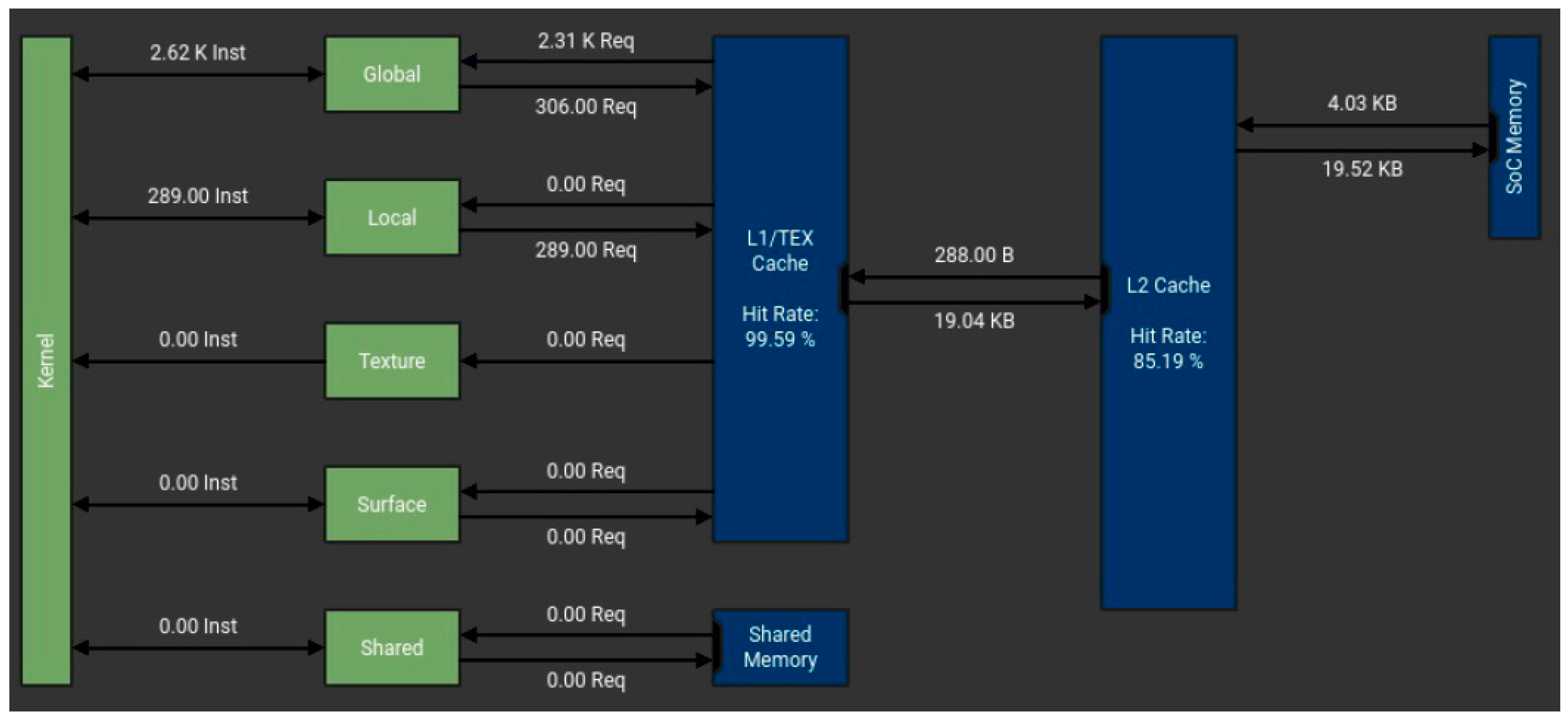
Memory is a very limiting factor for many applications, given that it exists in a limited quantity and is slower than CUDA units. By conducting a memory workload analysis of the classical algorithm,
Figure 2, 2.31 K reading and 306 writing requests were made from global memory, and 289 writing requests were performed from local memory to finish its execution. The four-section parallel implementation of the same algorithm requires only 135 reading and 17 writing requests to the global memory and 94 requests to local memory to accomplish its job. The local memory (viewed as a private storage for an executing thread) has the same latency as the global memory—this memory is visible to all threads running in the GPU. In a GPU system, the local and global memory reside off the GPU chip and have the highest latency.
From all the results presented above, only by relating these write/read operations performed by the two algorithms is it easy to see the superior efficiency of the novel algorithm presented in this study.
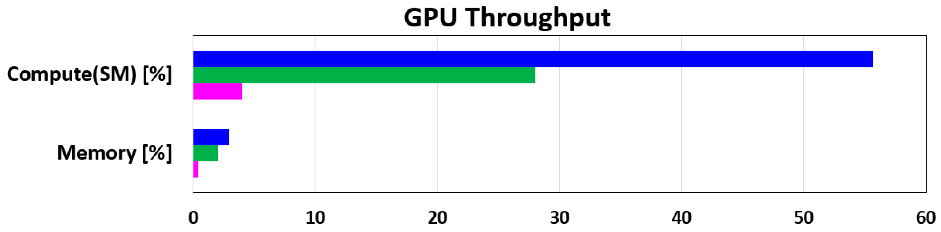
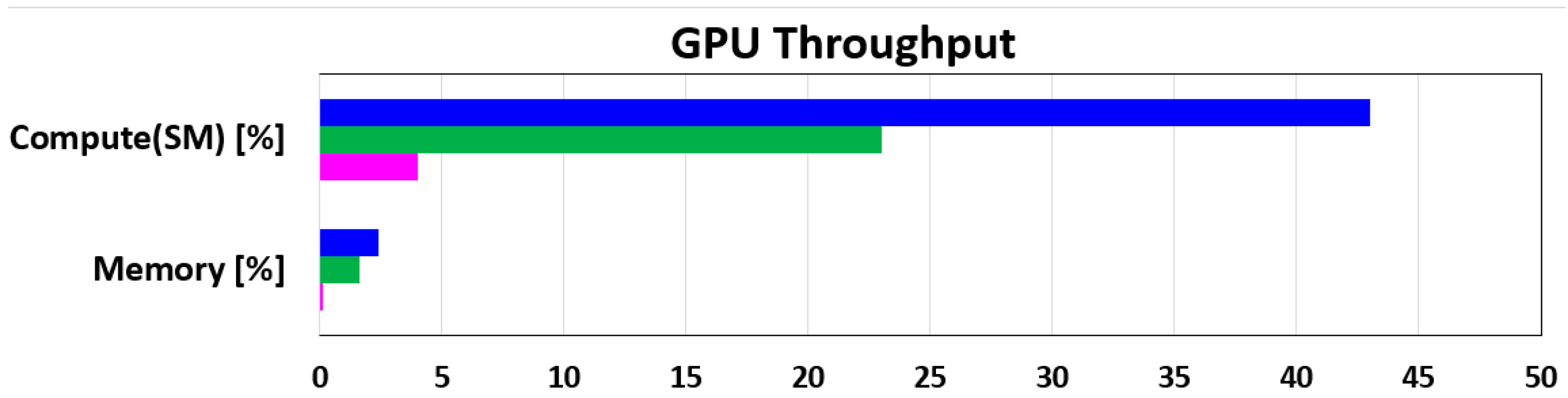
To view a high-level overview of the obtained performances for all three ways of implementing the DCT IV algorithm (classical implementation based on relation (1), novel algorithm with four sections, and novel algorithm with eight sections) in
Figure 3 and
Figure 4, the computation throughput and memory resources of the GPU are presented for a specific time frame presented in
Table 8. All of these data were recorded on the Jetson AGX Xavier development board using the NVIDIA Nsight Compute tool. The results from
Figure 3 and
Figure 4 are presented per SM unit and represent the achieved utilization percentage reported to the theoretical maximum limit. At 114.75 MHz, the classical implementation of the DCT IV algorithm obtained 3.76% of the overall compute throughput of an SM unit for 2.53 ms (
Table 8). In the same conditions, our four-section parallel implementation of the DCT IV algorithm generated a computational throughput of 28.05%, as compared with the classical implementation for only 156.45 us.
The theoretical speedup of an application when multiple cores are used is limited by the part of the task that cannot benefit from the improvement in the multiple cores. The novel algorithm was developed in such a specific way that a part of it can be easily split into four or eight different threads.
Table 9 presents the percentage of the algorithm that cannot be parallelized as a ratio between the execution time of this part and the total execution time. The results are presented for the Volta architecture (the GPU existing on Jetson AGX Xavier development board) for both parallel implementations (with four sections or with eight sections) and for the lowest acceptable working frequency of the GPU (114.75 MHz) and the highest working frequency of the GPU (1.377 GHz).
The execution time of a specific program section is composed of the times required to access memory for read/write operations and the time needed by the CUDA core to process the data. In our specific case, the part of the algorithm that cannot be parallelized is composed mainly of data initialization—matrix initialization, the initialization of the different cosine terms, and other elements necessary for the algorithm (see
Appendix B). In this section, there are very few mathematical computations. The sections of the algorithm that can be parallelized are dominated by mathematical calculations and fewer memory accesses. Once the CUDA core frequency increases from 114.75 MHz to 1.377 GHz, the instruction execution speed increases 12-times while the memory access time remains almost the same. This factor increases the proportion of the common part of the algorithm from 36.7% to 47.4% in the case of the algorithm with four sections and from 50.6% to 58.5% in the case of the algorithm with eight sections.
Due to the same process presented in the previous paragraph, the speedup factor is higher at lower frequencies and lower to the higher frequencies of the CUDA core units,
Table 4,
Table 5,
Table 6 and
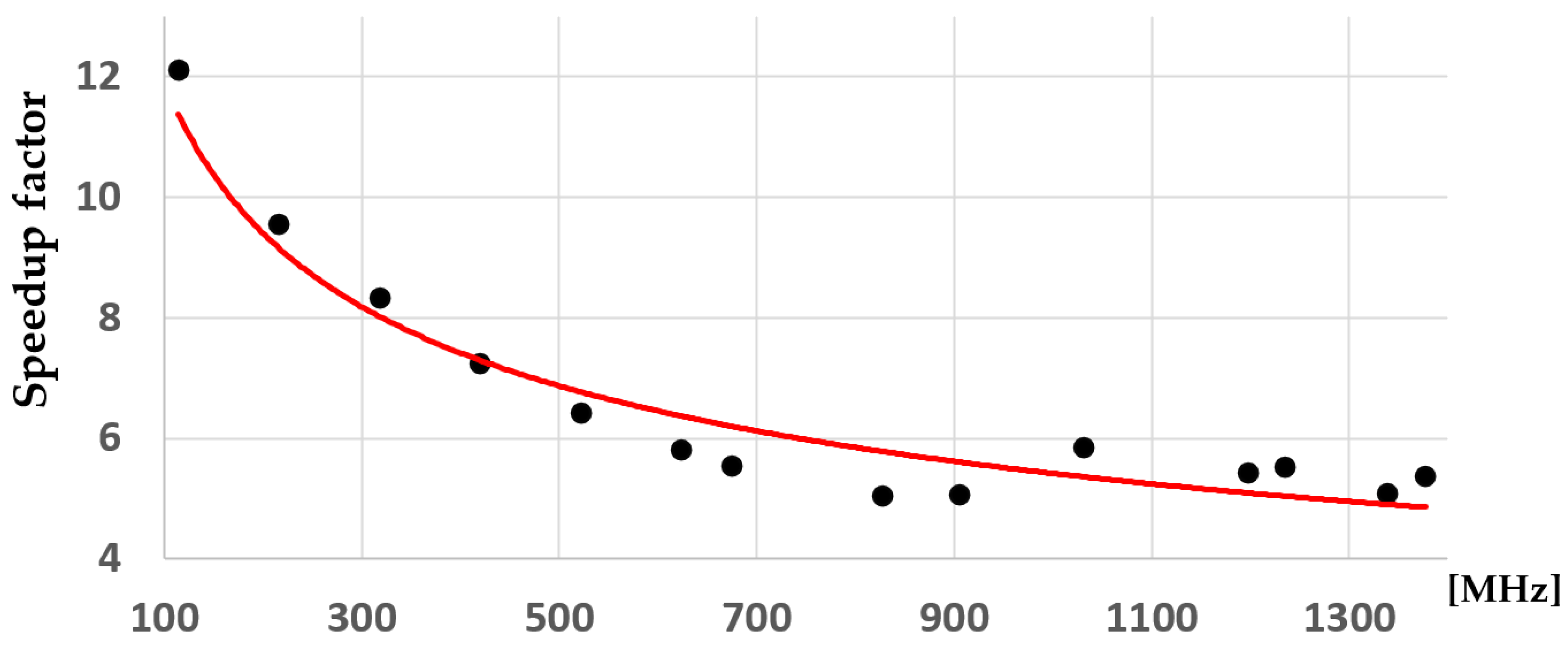
Table 7. To highlight the variation in the performance obtained by the new algorithm at different working frequencies of the GPU system, the graph in
Figure 5 was obtained.
As
Figure 5 illustrates, the speedup factor variation has no linear scale. The frequencies on which the determinations were made are the following ones: 114.75 MHz, 216.75 MHz, 318.75 MHz, 420.75 MHz, 522.75 MHz, 624.75 MHz, 675.75 MHz, 828.75 MHz, 905.25 MHz, 1032.75 MHz, 1198.5 MHz, 1236.75 MHz, 1338.75 MHz and 1377 MHz. These frequencies are several operating points preset by the manufacturer at which the GPU can work. The measurements presented in
Figure 5 were made under the same conditions as those in
Table 4,
Table 5,
Table 6 and
Table 7. The graph shows the average value and the standard deviation. Another interesting aspect can be seen from the figure: the variability in the determinations of the speedup factor for the proposed algorithm is high at low frequencies. Then, it decreases with the increase in frequency.
In the following analyses, a BFloat16 variable representation was used for the novel DCT IV algorithm implementation proposed in this study. The CUDA library supports this numerical implementation, and all the computational operations are supported in silicon in the frame of the Ampere architecture. The BFloat16 representation is used mainly to increase the calculation speed and to reduce the storage requirements of different types of algorithms.
From
Table 10 and
Table 11, a performance improvement of 1.21- up to 1.88-times was observed only by implementing the proposed algorithm using the BFloat16 numerical representation.
Overall, the performance improvements are between 16.38 and 22.5 for the novel DCT algorithm implemented in four sections and between 17.12 and up to 19.41 for the eight-section approach. Of course, the use of the BFloat16 representation also has disadvantages. Even if the dynamic range of the BFloat16 representation is identical to that of the float32 representation, the precision is limited to a maximum of three significant decimal digits. Depending on the field in which this novel DCT IV algorithm will be used based on a BFloat16 data representation, this low precision may represent a vital disadvantage or may not matter much. The data from
Table 10 and
Table 11 are presented so that a potential user of the algorithm can estimate the advantages brought by this algorithm implementation compared to the specific disadvantages generated by the loss of precision within its application.
6. Comparative Analysis
From the results presented in the previous section of this study, we observe the superior performances of the proposed algorithm compared to the performances obtained by a reference algorithm that implements the DCT IV transform using the implementation of relation (1). However, the natural question is: “How does this algorithm behave compared to other algorithms implemented by other researchers?” This section of the study will answer this question.
Comparing our results with those reported in the literature, we only notice that in [
30], an increase in the execution speed by a factor of 7.97 could be obtained. This result is close but inferior to those obtained in this work. However, this comparison is not very accurate because these performances were obtained on a RadeonTM HD 6850 GPU produced by the AMD company [
30]—a GPU based on a different architecture and operating philosophy compared to those of the NVIDIA company. As presented in
Table 4,
Table 5,
Table 6,
Table 7,
Table 8 and
Table 11, the performances of our algorithm, but not only, are strongly dependent on the architecture on which it works.
In [
37], Ryan et al. achieved a speed increase between 1.17 and 1.37 using an NVIDIA GTX280 graphics card. Unfortunately, this graphics card has a Fermi architecture before the Volta and Ampere architectures used in this work. Anyway, the performances are much lower than those obtained and reported in this study. The same can be said about the results presented in [
39]. This time, the performance increase was 2.46, but this was obtained on a Kepler-type architecture (prior to the Volta and Ampere architectures) in the coding of an entire frame—an operation composed both of the DCT transform and other operations (quantization, zigzag serialization, Huffman coding, color space conversion, etc.).
It is not straightforward to compare the results presented above [
30,
37,
39], with the results obtained by the novel algorithm introduced in this study—the test conditions are totally different (the architectures used, the working frequencies, the data buses between the GPU and the main processor, etc.). These results were presented only to observe the improvements obtained by the new algorithms compared to the previous DCT IV transform implementations used as a reference in these papers.
To correct this situation, two algorithms [
21,
40] were implemented on the Jetson AGX Xavier development board used in this study. The analysis methodology is similar to the one used in
Subsection 5 of this study. The reference algorithm directly implements relation (1) of the DCT IV algorithm. By implementing the algorithms presented in [
21,
40], we obtained the acceleration coefficient of the execution speed (speedup parameter from
Table 12 and
Table 13) due to these specific implementations, compared to the reference algorithm.
Table 12 and
Table 13 also show the number of global and local memory accesses each algorithm makes. Since the performance of the algorithms fundamentally depends on the GPU’s working frequency,
Table 12 presents the obtained performance for the minimum working frequency of the GPU. In contrast, in
Table 13, the performances are given for the maximum frequency accepted by the GPU.
By analyzing the data presented in
Table 13, we can draw the false conclusion that the algorithms proposed in this study [
21,
40] have superior performances compared to the algorithm presented in this study with four sections due to a shorter execution time. But these two algorithms work on 13 elements [
21,
40]. The algorithm proposed in this study works on a number of elements equal to 17. As a direct conclusion, the direct comparison of the execution times is not irrelevant. For this reason, we chose to compare the speed improvement obtained by all four DCT IV algorithms against a reference algorithm, that is, the classical implementation of DCT IV based on relation (1) on the same number of samples.
As we consider the number of operations executed by each processing element in parallel and considering that the length N is the same for all three algorithms, the number of multiplications M is 5, the number of additions/subtractions A is 29 and the number of shift operations that correspond to multiplications with ½ or ¼ is 18 for the proposed algorithm and M = 16 and A = 12 for the algorithms from [
21,
40].
From the data analysis presented in
Table 12 and
Table 13, it can be seen that the new proposed algorithm outperforms the algorithm presented in [
21] from all points of view—speedup (higher) and the number of memory access (lower).
The algorithm in [
40] implements DCT IV transform on six sections working in parallel. In the case of the algorithm presented in this study, it can be parallelized on four or eight independent parallel sections. The speed performance of the algorithm implemented on four and eight sections exceeds the acceleration factor obtained by the algorithm [
40] in all cases—5.41 and 8.08 versus 4.25 at the maximum working frequency of the GPU and, respectively, 12.1 and 14.41 versus 6.12 at the minimum operating frequency of the GPU.
7. Conclusions
The results presented in the previous sections show that the novel implemented DCT IV algorithm far exceeded our expectations. Due to the factorization method of the DCT transform, the reduced number of mathematical operations involved, and its parallel implementation, we obtained improvements in execution speed between 10.11- and 11.97- times for the implementation based on four sections (
Table 4 and
Table 5) and between 11.81- and 16.04-times in the case of implementing the DCT algorithm based on eight independent sections (
Table 6 and
Table 7). All these results were obtained based on the Ampere architecture. By using the numerical representation of the BFloat16 type, an existing representation that can be manipulated hardware only within the Ampere architecture, we will obtain an increase in performance between 1.21- and 1.88-times, in addition to the already existing one—
Table 10 and
Table 11.
The implementation of the new algorithm proposed in this study for the Volta architecture brought the following performance gains: (a) for the implementation of the algorithm based on the parallel execution of four sections, the increase in execution speed compared to the classical implementation of the DCT IV algorithm was between 5.41 and 12.1, (b) and in the case of the algorithm with eight sections, we obtained an increase in the execution speed between 8.08- and 14.41-times.
Also, comparing the novel algorithm directly against recent algorithms [
21,
40] under the same conditions, we notice that it surpasses them in all cases.
A disadvantage of this algorithm is that it can only be parallelized on four or eight different units. This is due to the mathematical method of factorization, which is the basis of its implementation.
This research aimed not to develop an algorithm that can efficiently use a GPU and fill out all its cores. But this is not a big problem for our algorithm. The DCT transform classical scenario usage is to be a component of the image compression algorithm. In such a case, it works on non-overlapping quadratic regions that, all together, make up the image. So, based on this approach, an ultra-HD image (3840 × 2160) can be split into more than 32,000 quadratic regions, and the DCT IV will be computed simultaneously in parallel on all cores of the GPU on each area. In this mode, many, if not all, CUDA units will be used.
In conclusion, we can say that the new algorithm introduced is a very high-performance one capable of obtaining remarkable accelerations in the execution speed of the DCT IV transform through a parallel implementation on four sections and based on the reduced number of mathematical operations. If the requirements compel an additional acceleration in the execution speed, the implementation based on eight parallel sections of this algorithm can be used.


