Article

Time-Delay Following Model for Connected and Automated Vehicles Considering Multiple Vehicle Safety Potential Fields

1
Shandong Key Laboratory of Smart Transportation, Jinan 250014, China
2
School of Information Engineering, Chang’an University, Xi’an 710064, China
3
School of Electronics and Control Engineering, Chang’an University, Xi’an 710064, China
*
Author to whom correspondence should be addressed.
Appl. Sci. 2024, 14(15), 6735; https://doi.org/10.3390/app14156735
Submission received: 12 June 2024 / Revised: 29 July 2024 / Accepted: 30 July 2024 / Published: 1 August 2024
(This article belongs to the Topic Vehicle Dynamics and Control)

Abstract

:
Connected and automated vehicles (CAVs) represent a significant development in the transport industry owing to their intelligent and interconnected features. Potential field theory has been extensively used to model CAV driving behaviour owing to its objectivity, universality, and measurability. However, existing car-following models do not consider the impact of time delays and the influence of information from multiple vehicles ahead and behind. This paper focuses on the driving-safety risks associated with CAVs, aiming to enhance vehicle safety and reliability during travelling. We developed a multi-vehicle car-following model based on safety potential fields (MIDM-SPF), taking into account the characteristics of multi-vehicle connected information and time delays. To enhance the model’s precision, real-world data from urban roads were employed, alongside an improved optimisation algorithm to fine-tune the car-following model. The simulation experiment revealed that MIDM-SPF significantly reduces stop-and-go traffic, thereby improving traffic flow stability in urban areas. Additionally, we validated the stability of our model under varying market penetration rates in large-scale mixed traffic. Our findings indicate that increasing the CAV proportion improves the stability of mixed traffic flows, which has important implications for alleviating traffic congestion and guiding the large-scale implementation of autonomous driving in the future.

1. Introduction

Potential field theory has gained prominence in modelling driving behaviour in traffic scenarios; it is valued for its objectivity, universality, and measurability. At the close of the 20th century, Khatib [1] pioneered the use of artificial potential field theory for robot movement, which subsequently found applications in cooperative control [2,3], path planning [4,5], and algorithm optimisation [6,7]. Motivated by these developments, numerous studies have adapted potential field theory for traffic flow research, yielding significant results. Li et al. [8] devised a visual stress energy field model to describe drivers’ visual perception and behavioural decision-making, classifying various driving risk levels. Semsar-Kazerooni et al. [9] employed a potential field function to design a novel collaborative adaptive cruise control strategy aimed at vehicle collision avoidance. Liu et al. [10] applied potential field theory to model dynamic traffic environments in road scenarios, developing a predictive control model encompassing an overall potential function and constraints. Their model was effective in controlling various driving behaviours such as lane keeping, lane-changing, following, and overtaking across different traffic scenarios. Xu et al. [11] combined the distance potential field with an artificial potential field to create a two-dimensional driving model, simulating turning behaviours at mixed-flow intersections with precision in scaling vehicle motion states. Ma et al. [12] examined the influence of surrounding vehicle potential field spacing on lateral acceleration and proposed a vehicle lane-changing time model for urban road b-type weaving sections using potential field theory. Their experiments successfully simulated the interplay between vehicle lane-change time, lateral, and longitudinal displacement. Joo et al. [13] designed a risk field representing vehicle conflict behaviour in highway driving, based on potential field theory, and established a probabilistic trajectory prediction model. Meanwhile, Cheng et al. [14] constructed an analytical model to assess the impact of scenario elements on driving behaviour using potential field theory. By integrating a hierarchical analysis method, they quantitatively evaluated the complexity of traffic scenes. These studies collectively demonstrate the utility of potential field theory in elucidating various driving behaviours and their interrelationships in complex traffic environments.
Microsimulation models for urban traffic flows typically employ vehicle-following behaviour modelling as a key application scenario [15]. Studying driving behaviour through various theoretical perspectives on vehicle-following remains an important aspect of micro traffic flow simulations. Over time, vehicle-following models have evolved into several notable categories: Gazis et al. [16] developed a classical GM car-following model based on the stimulus–response principle. Kometani et al. [17] introduced a safety distance model that takes into account the following distance. Michaels et al. [18] proposed a physiological–psychological model, defining a series of thresholds and expected distances to mirror human perceptions and reactions. Kikuchi et al. [19] employed artificial intelligence (AI) techniques to extract patterns of car-following behaviour from track data, resulting in an AI model. Bando et al. [20] created an optimised speed model using data such as preceding vehicle speed and gap distance. Wang et al. [21] proposed a cellular automaton model specifically for high-speed vehicle traffic flow. Further applications of potential field theory in this domain include the work of Yang et al. [22], who factored in the influence of lateral distance on continuous vehicle driving, proposing a car-following model based on potential field theory. Li et al. [23] introduced a simple model derived from the concept of a potential field, approached from a stimulus–response perspective. Jia et al. [24] established a molecular car-following model based on molecular interactions and wall potential functions, explaining the asymmetry in drivers’ following behaviour and their acceleration/deceleration actions at various distances. In multi-vehicle-following scenarios, Zhang et al. [25] explored the robust formation control of unmanned surface vehicles using vehicle safety distance, employing potential field theory for formation-switching tasks. Shen et al. [26] considered data from multiple preceding vehicles and introduced a vehicle time headway strategy using potential field theory, enhancing driving and riding comfort by adjusting vehicle speed, acceleration, and following distance. However, many of these models still lack real vehicle-following data or have not undergone calibration for model parameters. Consequently, the capability of these models in controlling vehicle-following behaviour warrants further validation.
This study presents a car-following model for CAVs, grounded in safety potential fields, with a focus on vehicle-following behaviour. This model accounts for the time delay in information reception and processing, as well as safety potential field data that reflect the acceleration characteristics of vehicles. The calibration of relevant parameters within this model utilises real vehicle data from urban roads and is enhanced through advanced arithmetic optimisation algorithms. A notable feature of this model is the incorporation of specific target-state information, which significantly enhances the stability of the subject vehicle during following behaviour. This aspect proves particularly beneficial for temporary queues of autonomously driven cars, augmenting both the stability and operational efficiency of these queues, as well as the overall traffic flow. The remaining sections of this paper are organised as follows. Section 2 provides a brief literature review. Section 3 elaborates on the traffic scenario, outlining the methodology for constructing a car-following model using safety potential fields and the approach for calibrating model parameters, followed by the validation of the model’s stability. Subsequent numerical simulations are conducted, encompassing the parameter calibration of the model, dynamic performance analysis, and simulations under various market penetration rates. The final section provides a comprehensive summary of this study.

2. Literature Review

2.1. Safety Potential Fields

The safety potential field (SPF) model is a concept used in the field of autonomous vehicles and robotics to enhance safety and navigation efficiency. In practical terms, this model works by calculating the forces acting on a vehicle based on its proximity to objects or boundaries. When a vehicle approaches an obstacle, the repulsive force from the obstacle pushes the vehicle away to prevent collisions. By employing the SPF model, autonomous vehicles can navigate complex environments with greater safety and efficiency. This model is crucial for ensuring that vehicles can move smoothly, avoid collisions, and reach their destinations effectively [27].
The SPF leverages field theory to encapsulate risk factors originating from drivers, vehicles, road conditions, and other traffic factors. This approach is instrumental in assessing potential driving risks in actual traffic scenarios and forecasting trends in driving safety due to dynamic changes [28]. Building on this concept, Wang et al. [29] took into account a comprehensive model of human–vehicle–road interaction and introduced a vehicle collision warning algorithm based on the driving-safety field model. Their work delved into both the modelling and practical application of driving-safety field theory. Li et al. [30] crafted a dynamic authority allocation strategy between the driver and the trajectory tracking controller, based on game theory and driving-safety field theory. They developed a safety control model for assessing driver risk, with experimental results indicating that their strategy effectively aids vehicles in achieving robust obstacle avoidance performance. The strategy also empowers the controller to proactively take control of the vehicle, guided by the assessment of driving risk under current conditions.
Further advancing this field, Li et al. [31] proposed a risk perception and warning strategy based on a safety potential field model. This model delineates the spatial distribution of vehicle driving risk by creating a dynamic model of vehicle operation. Additionally, Li and Gan [32] established a lane-changing model using safety potential field theory. Numerical simulation analysis showed that this model proficiently reflects the impact of various motion parameters on lane-changing results. Expanding their research, they [33] also developed a macroscopic model for heterogeneous traffic flow in an interconnected automated environment, based on safety potential field theory. Their results underscored that the penetration rate of such technology significantly impacts road capacity, highlighting the model’s relevance in understanding and managing complex traffic dynamics. Hence, we integrate SPF with microscopic simulation models to comprehensively describe microscopic driving behaviours using a dynamic driving risk potential field, further characterising the level of safety risk during the driving process.

2.2. Car-Following Behaviour Modelling of SPF

As intelligent driving systems evolve, technologies such as vehicle-to-vehicle (V2V), vehicle-to-infrastructure (V2I), advanced driver-assistance systems (ADAS), automated emergency braking systems (AEBS), LIDAR, and GPS are enabling vehicles to acquire increasingly precise real-time data about their surrounding human–vehicle environment. This advancement facilitates early warning, assistance, and intelligent decision-making functions for driving operations [34]. Li et al. [35] developed a dynamic driving risk potential field model in a connected and automated driving environment. This model thoroughly considers the dynamic effects of vehicle acceleration and steering angle and calibrated its parameters using NGSIM data in traffic scenarios. In addition, they [36] integrated graph theory with safety potential field theory to devise a queue formation and optimisation model for CAVs under varying vehicle distributions, with simulations indicating the model’s efficacy in forming a collision-free queue swiftly. Wu et al. [37] introduced a risk assessment model based on potential field theory, designed to quantify driving risks. This model demonstrated strengths in risk perception and response, vehicle-tracking trajectory, and speed estimation.
These fields collectively describe the safety risks for CAVs in motion. Jia et al. [38], focusing on the autonomous decision-making capabilities of CAVs by sensing their surroundings, established a safety potential field model that includes lane-marking, a road boundary, and vehicle potential fields. Li et al. [39] addressed the microscopic state evolution mechanism of mixed traffic flow, comprising CAVs in an intelligent connected environment. They proposed a mixed traffic flow safety potential field model based on potential field theory that can adjust vehicle acceleration in real-time according to the potential field distribution and more accurately represent the actual following state. Ma et al. [40] designed a risk potential field between interactive and automated vehicles, formulated a real-time risk assessment model for weaving areas, and introduced an alternative safety measure index for vehicle operation risks. However, these models have not accounted for the impact of time delays and the influence of information from multiple vehicles ahead and behind in the car-following model, indicating a potential area for further refinement in these models. Table 1 presents a summary of the car-following behaviour modelling works related to SPF found in the literature, with the final row highlighting the unique contribution of this study.

3. Methodology

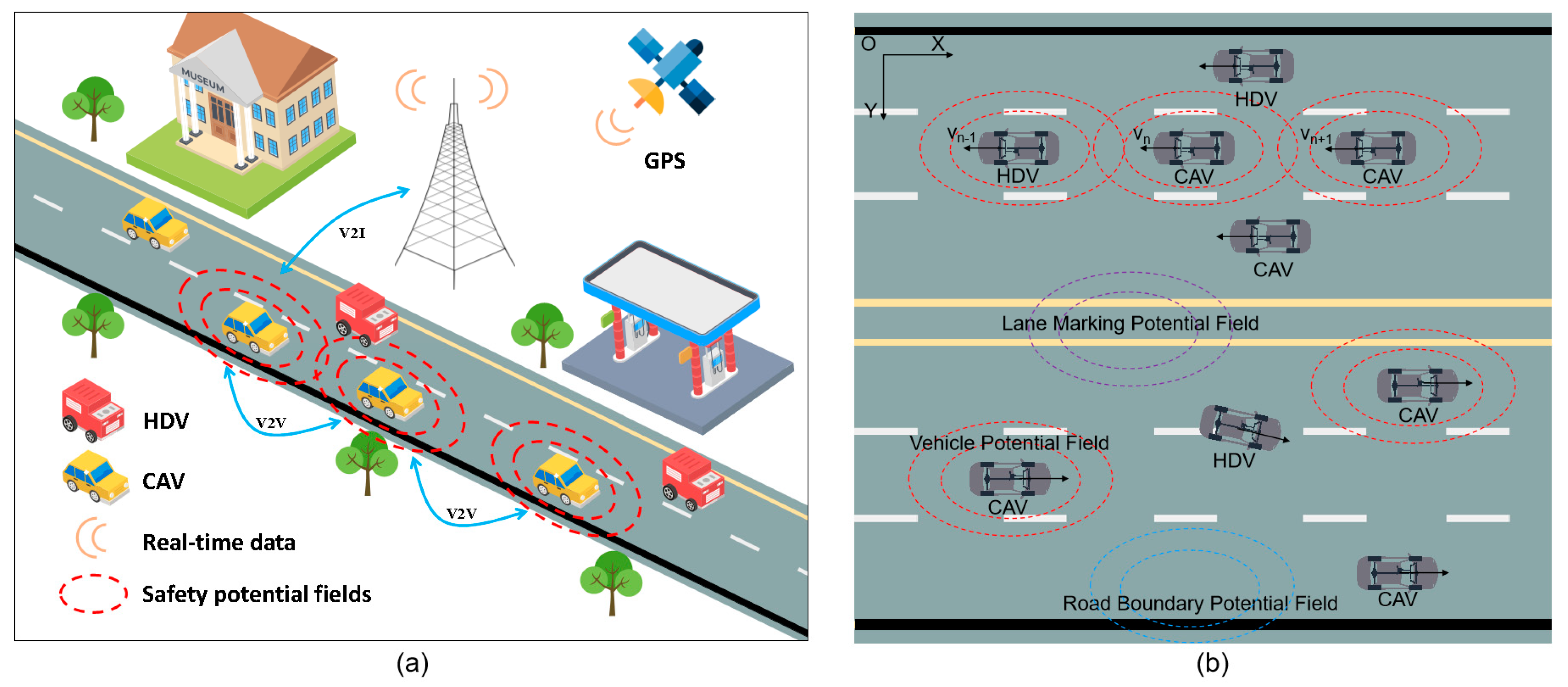
3.1. Car-Following Model Based on Safety Potential Field

From the perspective of physics, a field can be defined as a space where objects in specific states exert interaction forces on other objects without physical contact over a certain spatial distance. The varying relative positions of these objects lead to differences in the interaction of forces, generating potential energy related to attributes such as distance, size, and weight. In this way, fields and potentials with different properties combine throughout the physical space, displaying the capacity for objects to interact with one another. Similarly, in traffic scenarios, there is a correspondence between vehicle driving behaviour and potential field theory. In car-following scenarios, sudden disturbances can prompt notable oscillations in vehicle speed due to the requirement for maintaining safe driving distances. Vehicles constantly adjust their speeds to preserve a safe distance from the vehicle ahead, a dynamic adjustment strategy akin to the influence of force in a potential field, which ultimately contributes to traffic flow stability. This also reflects the driving risks that emerge as vehicles respond to changes in scenario elements during motion.
In mixed traffic environments featuring CAVs and human-driven vehicles (HDVs), CAVs can obtain extensive state information about the surrounding environment, including their own locations, lane lines, and information about surrounding vehicles. In these traffic scenarios, any element impacting a vehicle’s driving state can be considered a field source in the physical space. The safety potential field characterises driving safety in car-following scenarios based on the interaction forces of these elements. To analyse the amalgamation of vehicles, roads, and environmental elements in coupled scenarios in a layered manner, this study adopts an adaptive layered model for scenario representation, as per Menzel et al. [41]. Figure 1a,b illustrates a typical car-following scenario, comprising three key elements: lane-marking lines, road boundary lines, and vehicles. Consequently, in the traffic environment, CAVs are influenced by the potential fields of lane-marking lines, road boundary lines, and other vehicles, denoted as UL, US, and Uv, respectively. The safety potential field is calculated using (1).
U t o t a l = w L U L + w s U s + w v U v ,
where UL represents the lane-marking field, US denotes the road boundary field, Uv is the vehicle field, and wL, ws, and wv are their respective weight coefficients. For the SPF model, derivation, and simulation concerning lane-marking lines, road boundary lines and other vehicles, please refer to Appendix A, specifically Appendix A.1.
Assuming all vehicles travel along the road’s centreline, the lane-marking and road boundary potential fields become irrelevant. Consequently, there is no need to consider lane-changing behaviour or vehicle deviation angles in this scenario. The intensity of the vehicle potential field exerted by the (ni)th and (n + j)th vehicles on the nth vehicle can be expressed as follows. Figure 2 illustrates a multi-vehicle car-following scenario involving n + j vehicles (where both n and j > 0). The distance between the (ni)th and nth vehicle is denoted as x i , while the distance between the (n + j)th and the nth vehicle is x j .
U V n i , n = M n i λ e a n i k n i , n k n i , n k n i , n = M n i λ e a n i + v n i x i · s 0 k n i , n k n i , n ,
U V n + j , n = M n + j λ e a n + j k n + j , n k n + j , n k n + j , n = M n + j λ e a n + j + v n + j x j · s 0 k n + j , n k n + j , n ,
where M n i and M n + j represent the actual weight of the (n − 1)th and (n + 1)th vehicles, and v n i and v n + j are their respective velocities. k n i , n and k n + j , n denote the distances from the nth vehicle. The field force F experienced by vehicles in a real car-following state indicates the level of safety risk, with higher risks leading to stronger field forces. This concept draws an analogy to the calculation formula for electric field force, leading to an expression for the field force exerted on the nth vehicle by the (ni)th and (n + j)th vehicles.
F n i , n = U V n i , n M n e v n = M n i λ e a n i + v n i x i · s 0 M n e v n ,
F n + j , n = U V n + j , n M n e v n = M n + j λ e a n + j + v n + j x j · s 0 M n e v n ,
where Mn denotes the actual weight of the nth vehicle. vn represents the velocity of the nth vehicle. For the (ni) and (n + j) vehicles, the accelerations a n i , n and a n + j , n under the action of the field forces F n i , n and F n + j , n are expressed as:
a n i , n = F n i , n M n = M n i λ e a n i + v n i x i · s 0 e v n ,
a n + j , n = F n + j , n M n = M n + j λ e a n + j + v n + j x j · s 0 e v n ,
According to the previous description of the safety potential field, the field forces within a certain range influences the vehicles. In larger distances between preceding and following vehicles, the intelligent driver model (IDM) is employed to capture the car-following behaviour characteristics [42,43]. This includes the vehicle’s response to acceleration and deceleration in both free-flow and congested flow conditions. The car-following model based on the safety potential field is expressed as:
d v n t + t d d t = a 0 1 v n t v 0 4 s n * t s n t 2 + γ a n i t a n i , n t + μ a n + j t a n + j , n t = a 0 1 v n t v 0 4 s n * t s n t 2 + γ i = 1 p a n i t M n i λ e a n i + v n i x i · s 0 e v n + μ j = 1 q a n + j t M n + j λ e a n + j + v n + j x j · s 0 e v n ,
s n * t = s 0 + T v n t + v n t Δ v t 2 a 0 b ,
where a 0 and v0 represent the maximum acceleration and desired velocity of the following vehicle in free-flow conditions, and vn(t) is the velocity of the following vehicle at time t. s n * t is the desired headway, sn(t) is the actual headway, T is the safe time headway, and Δ v t the velocity difference between the following and leading vehicles. b indicates the comfortable deceleration, while p and q are the numbers of preceding and following vehicles, respectively. td is the time delay for information reception and processing. γ and μ represent the sensitivity coefficients of the safety potential field.

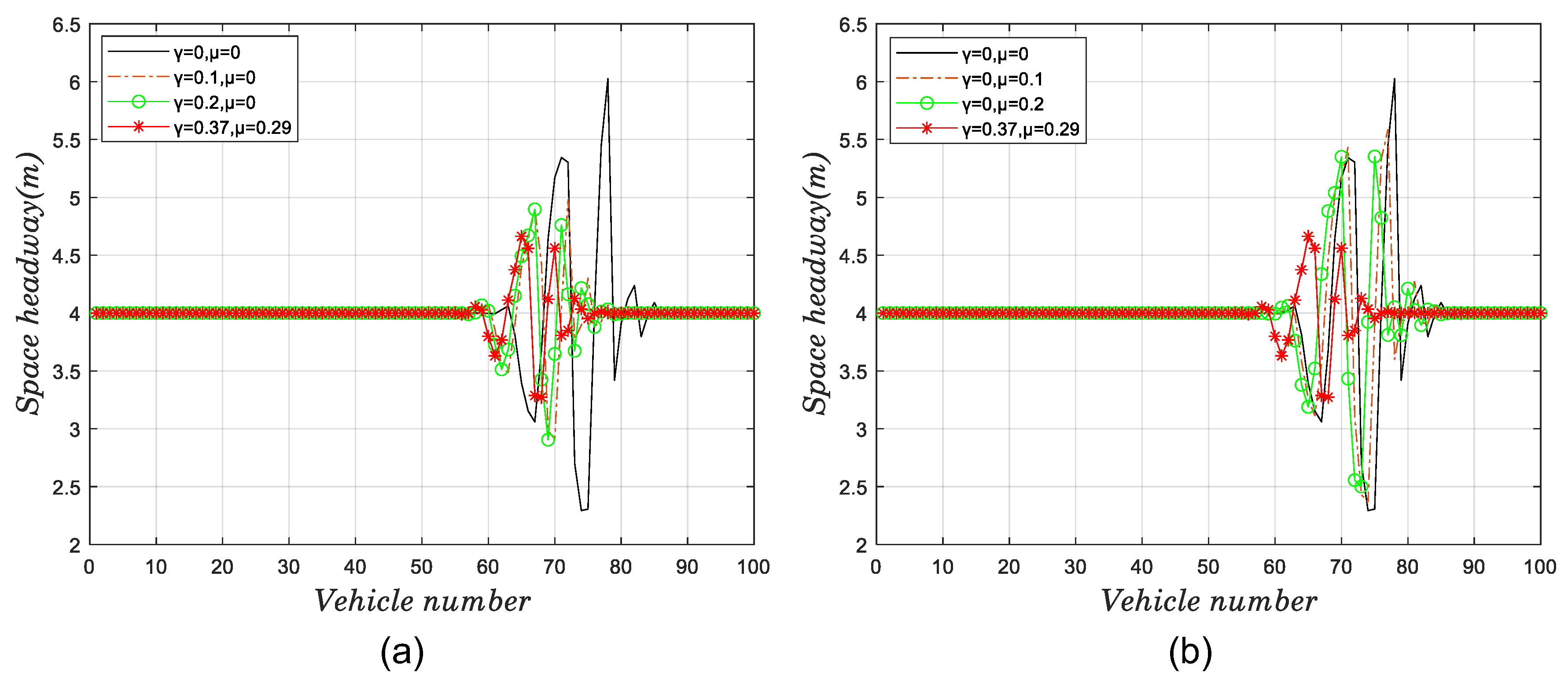
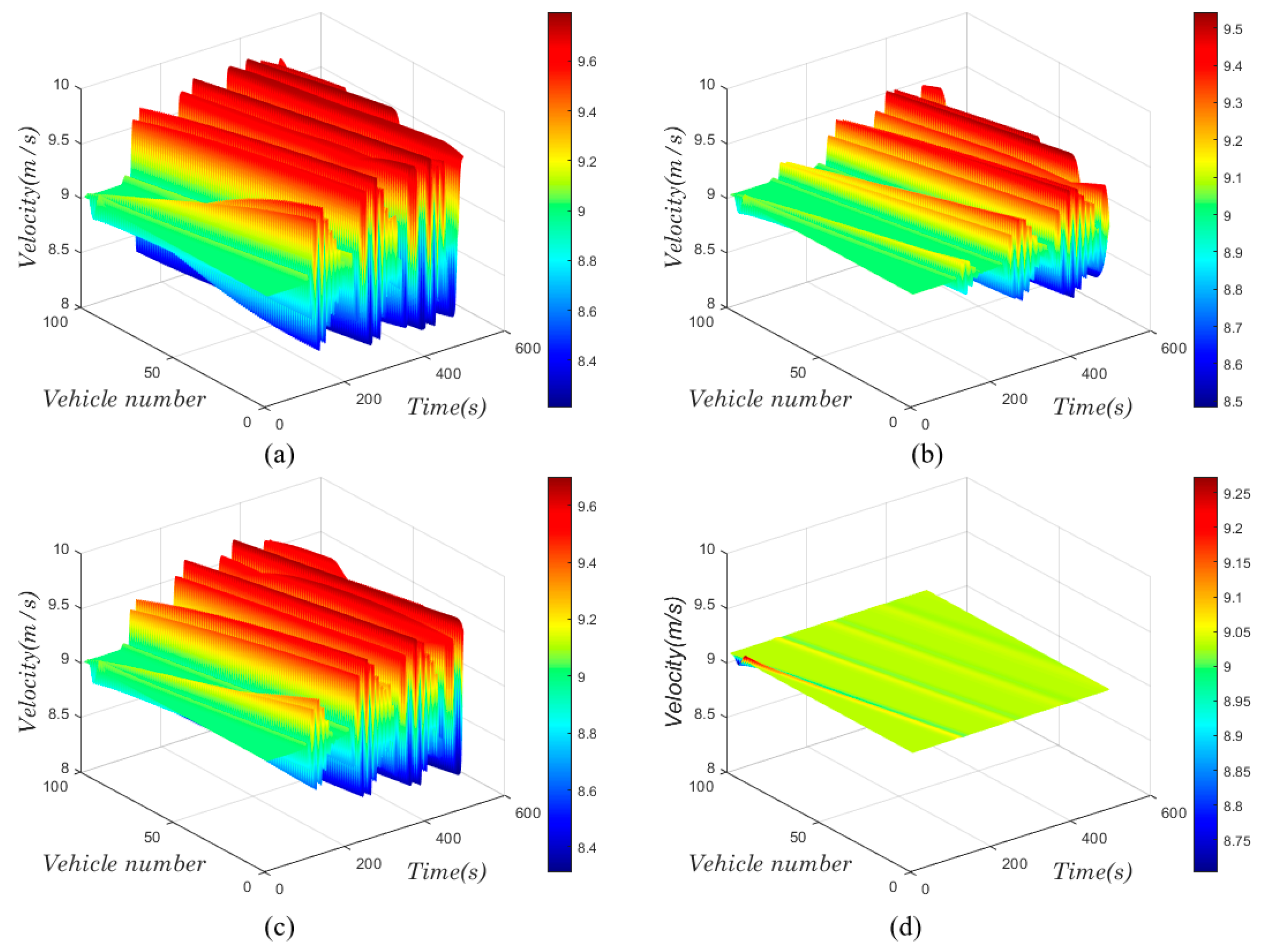
3.2. Stability Analysis

Stability analysis is vital for car-following models. Zhao et al. [44] utilised frequency-domain scanning methods to analyse the stability of driver characteristics and controller gains. Wang et al. [45] investigated the stability of car-following models through frequency-domain analysis tools and stochastic process theory, while Wang et al. [46] derived a characteristic equation to describe the evolution of traffic density waves via nonlinear analysis. In this paper, we analyse the stability of the MIDM-SPF model using linear stability theory and simplify (8) as follows:
d v n t + t d d t = f n s t , v n t , Δ v t , a n i t , a n + j t , v n i t , v n + j t , Δ x i , Δ x j ,
We assume that s ¯ represents the average headway between neighbouring vehicles in uniform flow and v ¯ denotes the vehicles’ velocity in this flow. Initially, all vehicles travel with identical headway and velocity; hence, the position of vehicles in uniform flow can be expressed as follows:
x ¯ n t = N n s ¯ + v ¯ t ,   n = 1,2 , 3 , N ,
Assuming y n t is the disturbance generated by vehicle n at time t, we add this disturbance to (11).
y n t = c e ω α k n + z t = x n t x ¯ n t ,   y n t 0 ,
where α k = 2 π k N k = 0,1 , , N 1 is a constant. Taking the second derivative of both sides of (12), we obtain
y n t + t d = x n t + t d x ¯ n t + t d = d v n t + t d d t ,
Substituting (10) into (13), we obtain
y n t + t d = f n s t , v n t , Δ v t , a n i t , a n + j t , v n i t , v n + j t , Δ x i , Δ x j ,
Linearize Equation (14) and substitute y n t = c e ω α k n + z t and y n t = z c e ω α k n + z t into the difference equation. Rearrange terms, simplify, and expand in a power series to obtain the stability condition as shown in Equation (15). Here, traffic flows become unstable when z 2 < 0 in response to small perturbations and stabilise when z 2 > 0 . For a detailed proof of the stability analysis, please refer to Appendix A, Appendix A.2.
t d 2 < 1 f n a n i f n a n + j f n v n + f n v n i + f n v n + j + f n Δ v i f n v n i + j f n v n + j f n s + i f n Δ x i j f n Δ x j + f n v n + f n v n i + f n v n + j f n s + i 2 f n Δ x i + j 2 f n Δ x j 2 f n s + i f n Δ x i j f n Δ x j 2 ,
Combining Equation (8) yields results for f n s , f n v n , f n Δ v , f n a n i , f n a n + j , f n v n i , f n v n + j , f n Δ x i and f n Δ x j . Substituting these results into Equation (15) gives the stability condition as shown in Equation (16).
t d 2 < 0.5 · 1 γ i = 1 p 1 + M n i λ e v n + v n i x i · s 0 e a n i μ j = 1 q 1 + M n + j λ e v n + v n + j x j · s 0 e a n + j a 0 2 v 0 v n t v 0 3 + T s 0 + T v n t s n 2 t + γ i = 1 p M n i λ e a n i + v n i x i · s 0 e v n + μ j = 1 q M n + j λ e a n + j + v n + j x j · s 0 e v n + s 0 + T v n t v n t s n 2 t a 0 b + i γ i = 1 p M n i λ e a n i + v n x i · s 0 e v n i j μ j = 1 q M n + j λ e a n i + v n x j · s 0 e v n + j 2 a 0 s n t s 0 + T v n t s n t 2 + i γ i = 1 p M n i λ e a n i + v n i S 0 Δ x i 2 e v n j μ j = 1 q M n + j λ e a n + j + v n + j S 0 Δ x j 2 e v n + a 0 2 v 0 v n t v 0 3 + T s 0 + T v n t s n 2 t + γ i = 1 p M n i λ e a n i + v n i x i · s 0 e v n + μ j = 1 q M n + j λ e a n + j + v n + j x j · s 0 e v n × 2 a 0 s n t s 0 + T v n t s n t 2 + i 2 γ i = 1 p γ i = 1 p M n i λ e a n i + v n i S 0 Δ x i 2 e v n + j 2 μ j = 1 q M n + j λ e a n + j + v n + j S 0 Δ x j 2 e v n 2 a 0 s n t s 0 + T v n t s n t 2 + i γ γ i = 1 p M n i λ e a n i + v n i S 0 Δ x i 2 e v n j μ j = 1 q M n + j λ e a n + j + v n + j S 0 Δ x j 2 e v n 2 ,
Following the stability condition (16), we obtain the stability curve for V-T by setting parameters a 0 = 2 , v 0 = 10 , b = 1.5 , p = 1, and q = 1 , using additional parameters from Table A2. Figure 3, which demonstrates the stability curves for different values of γ and μ at t d of 0 and 0.15 [47], reveals that the stability curves decrease as γ and μ increase, indicating that considering the safety potential field of leading and following vehicles can improve traffic flow stability. Furthermore, at identical γ and μ values, the unstable region for t d = 0.15 is larger than t d = 0 , suggesting that accounting for time delays can alter a vehicle’s motion state, thus impacting traffic flow stability.

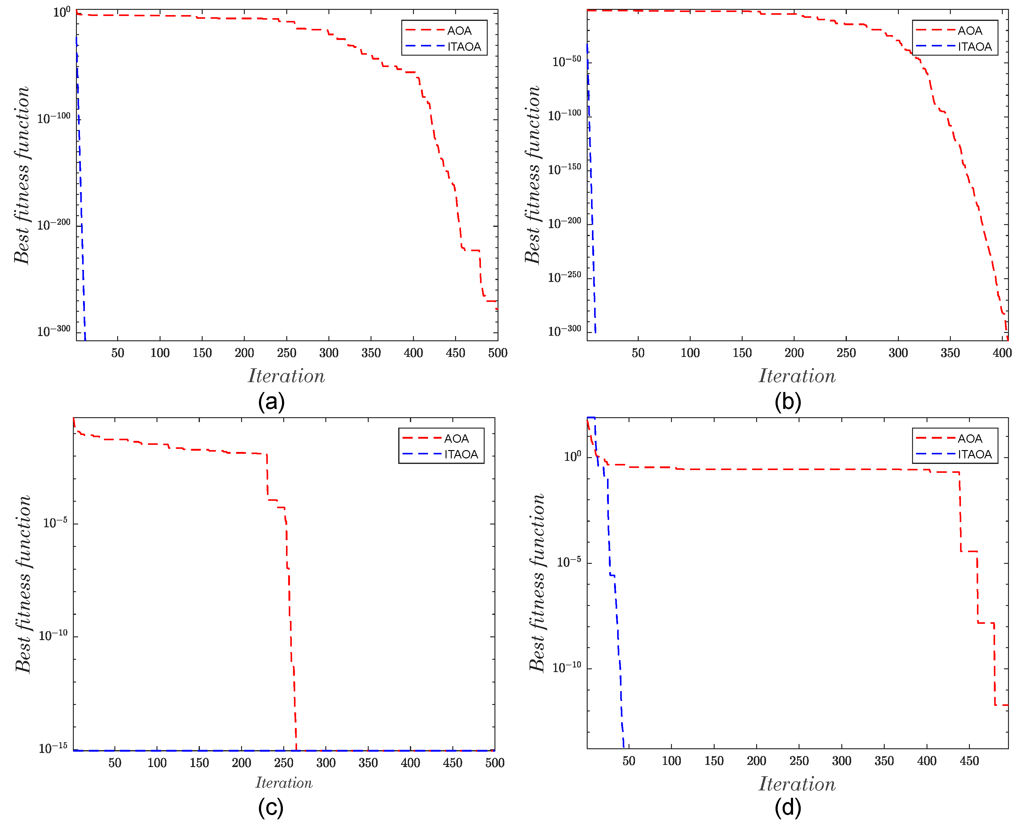
3.3. Calibration of the Model Parameter

The arithmetic optimisation algorithm (AOA), introduced by Abualigah et al. [48], is an innovative intelligent optimisation algorithm. It leverages the functionalities and application processes of arithmetic operators for solving arithmetic problems. The AOA is distinguished by its straightforward operations, brief optimisation duration, and high accuracy, rendering it highly suitable for applications such as neural network parameter optimisation [49] and optimal placement searching [50]. The algorithm initialises the population using a random number generation process:
Z N × D = r a n d N , D × ( U N , D L N , D ) + L N , D ,
where N represents the number of particles and D the dimensions to be explored or developed. Z d n represents the value of the n th solution in the d th dimension, with U and L representing the upper and lower value limits, respectively.
Following initialisation, the AOA employs the math optimiser accelerated (MOA) for numerical calculations, determining whether to enter the exploration (exp) or development (dev) phase:
M O A I t e r = I t e r × M m a x M m i n M a x I t e r + M m i n ,
γ 1 > M O A ,     exp γ 1 M O A ,     dev ,
where Iter signifies the iteration number, a represents the maximum iterations, with M m a x and M m i n being the MOA’s maximum and minimum values, respectively. γ 1 is a random number in the range [0, 1].
During the exploration phase, division and multiplication operations facilitate a global search. These operators, due to their high discreteness, are apt for global exploration. The exploration method is described by (20):
M O A Z d n I t e r + 1 = Z B I t e r / M O P + ϵ × U d L d × σ 1 + L d ,     γ 2 < 0.5 Z B I t e r × M O P × U d L d × σ 1 + L d ,     γ 2 0.5 ,
where Z d n I t e r + 1 is the updated position of the nth solution in the dth dimension, and Z B I t e r is the position of the current best solution. ϵ , U d , and L d represent the minimum integer, maximum and minimum values in the dth dimension. σ 1 signifies a control parameter for the search phase, typically set at 0.499. γ 2 is a random number in [0, 1]. The MOP calculation is expressed in (21), with the sensitivity parameter set as follows:
M O P ( I t e r ) = 1 I t e r 1 α M a x I t e r 1 α ,
In the development phase, addition and subtraction operations focus on local development. These operators, with their low discreteness, enable in-depth local development. The development method is outlined in (22):
Z d n I t e r + 1 = Z B I t e r M O P × U d L d × δ 1 + L d ,   γ 3 < 0.5 Z B I t e r + M O P × U d L d × δ 1 + L d ,   γ 3 0.5 ,
where γ 3 is a random number in [0, 1]. δ 1 is a design parameter that varies with each iteration, thus helping to break out of local optima.
During the actual calibration process, the initialisation of AOA with random numbers resulted in prolonged optimisation times, reduced accuracy, and difficulties in escaping local minima or boundary values. To overcome these challenges, this paper incorporates chaotic mapping to enhance the randomness, sensitivity, and exploration capabilities of the algorithm, specifically targeting the issues arising from random number initialisation. However, the circular chaotic mapping did not yield uniformly distributed initial solutions. Consequently, an improvement to the circular chaotic mapping is introduced.
The original circular chaotic mapping is outlined in (23).
Y k + 1 n = m o d ( Z k n + 0.2 0.5 0.2 π sin 2 π · x n , 1 ) ,
To ensure a more uniform distribution of chaotic values, we propose an improved version of the circular chaotic mapping, detailed in (24). This improvement ensures that chaotic values are more evenly spread across the entire range, while maintaining the explorative and stable properties of the original mapping.
Y k + 1 n = m o d ( 3.85 Z k n + 0.4 0.7 3.85 π sin 3.85 π · x n , 1 ) ,
where Y k + 1 n are chaotic sequences for the interval [0, 1]. n = 1,2 , 3 , N and k = 1,2 , 3 , D 1 . An inverse mapping is then performed to obtain the initial position of the population, as shown in Equation (25).
Z d n = Y k + 1 n × ( U N , D L N , D ) + L N , D ,
Moreover, the MOA value is crucial in determining whether the AOA transitions into global exploration or local development phases. A high MOA value enhances local development but may impede global exploration, potentially leading to the algorithm becoming trapped in local optima. Conversely, a low MOA value amplifies global exploration at the expense of local development, thereby extending optimisation times. To address this, this paper introduces a tangent factor to modulate the optimisation step size during algorithm iterations, as shown in (26):
T M O A = M m i n + M m a x M m i n × t a n π 2 × I t e r M a x I t e r ,
The efficacy of the improved tangent arithmetic optimisation algorithm (ITAOA) was evaluated against the standard AOA using unimodal functions (F1 and F2) and multimodal functions (F3 and F4) as benchmark functions, as outlined in [51]. The functional expressions for these benchmarks are provided in Table 2.
Figure 4 demonstrates that across all four benchmark functions, the ITAOA consistently outperforms the AOA in terms of fitness values and optimisation convergence speed. The ITAOA not only optimises faster and more accurately but also exhibits remarkable stability across different test functions. Contrary to the AOA, which shows considerable variation in convergence speed and optimisation accuracy, the ITAOA consistently achieves comprehensive global searches, thorough local development, and efficient termination upon locating the optimal solution, regardless of whether it is dealing with low-dimensional unimodal or high-dimensional multimodal functions.

4. Results

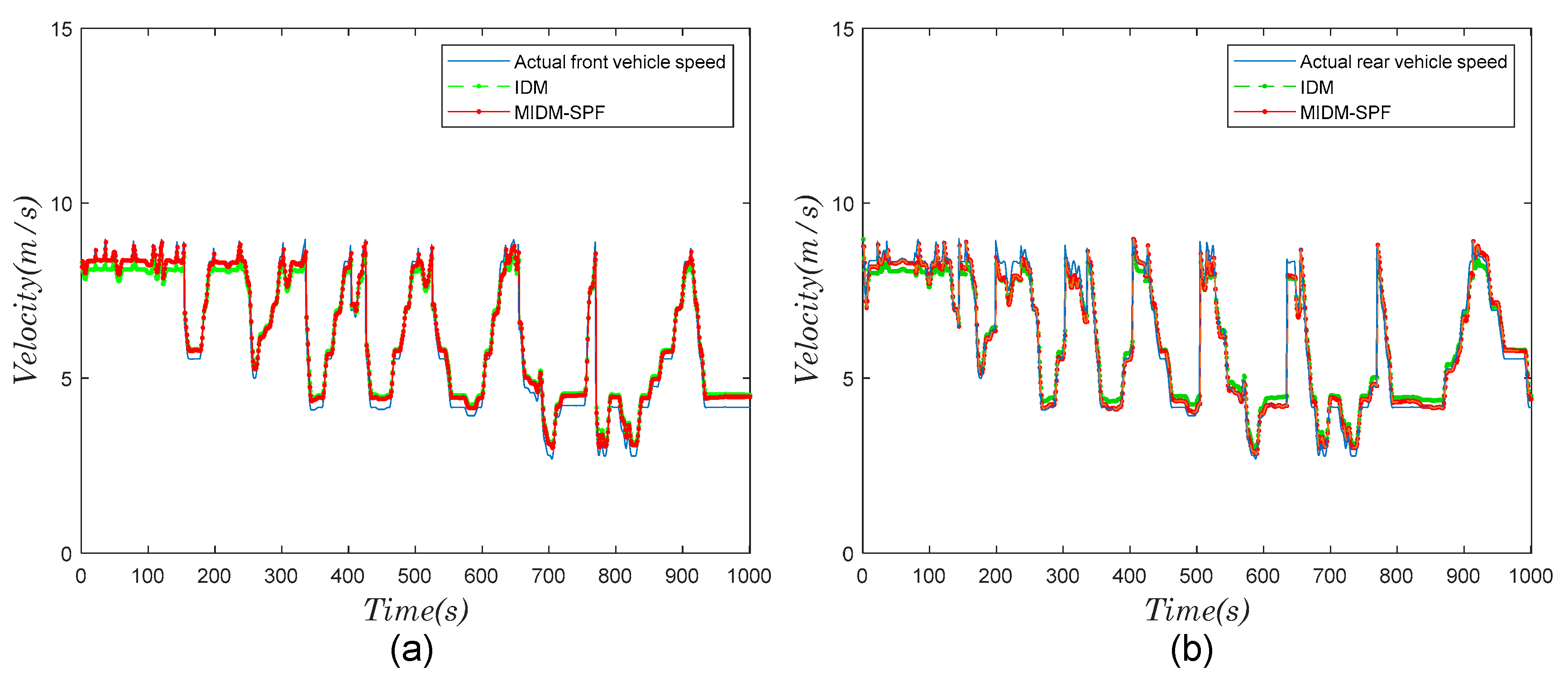
4.1. Model Calibration and Validation

In the context of a car-following scenario, variations in parameters significantly impact the vehicle’s motion state, and the driving behaviour adapted to the traffic scenario differs accordingly. In this paper, for the car-following model involving multiple vehicles within a safety potential field, the ITAOA was employed for parameter calibration owing to its superior convergence speed and optimisation accuracy, which are more in line with the calibration requirements of this model. Actual car-following data, specifically from the acceleration and deceleration processes on urban roads, were selected for calibrating the model. The calibration results of the MIDM-SPF model are presented in Table 3, with the key parameters γ and μ being 0.37 and 0.29.
To evaluate the proposed model in this paper effectively, the IDM was also calibrated using the same dataset. The final trajectory results of both the MIDM-SPF and the IDM were compared, as illustrated in Figure 5. Figure 5a,b display the differences between the estimated trajectories of the leading and following vehicles and the actual data for both models. In these figures, the blue line signifies the actual trajectory of the following vehicle in the car-following scenario, the green dashed line represents the trajectory estimated using the IDM, and the red solid line depicts the trajectory based on the MIDM-SPF model.
From the comparison, both the MIDM-SPF and IDM models did not perfectly match the real data. However, the estimated trajectory trends and errors of both models were within a reasonable range. To further compare the models’ effectiveness, key metrics such as the mean squared error, mean absolute error, and goodness of fit for these models on the dataset are summarised in Table 4. Evidently, the MIDM-SPF model demonstrates higher accuracy in terms of error precision compared to the IDM, with its goodness of fit being 2.3% higher than that of the traditional model. This finding suggests that the fitting performance of the improved MIDM-SPF model is better than the original IDM.

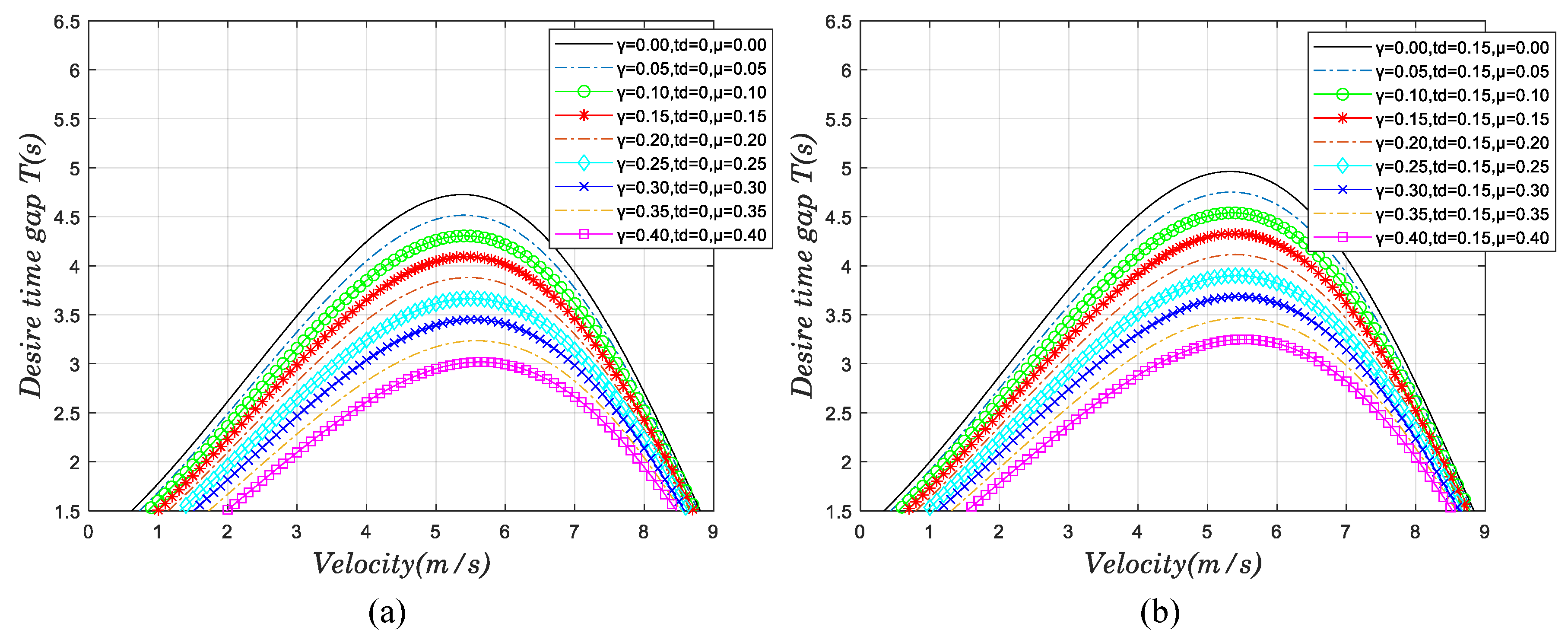
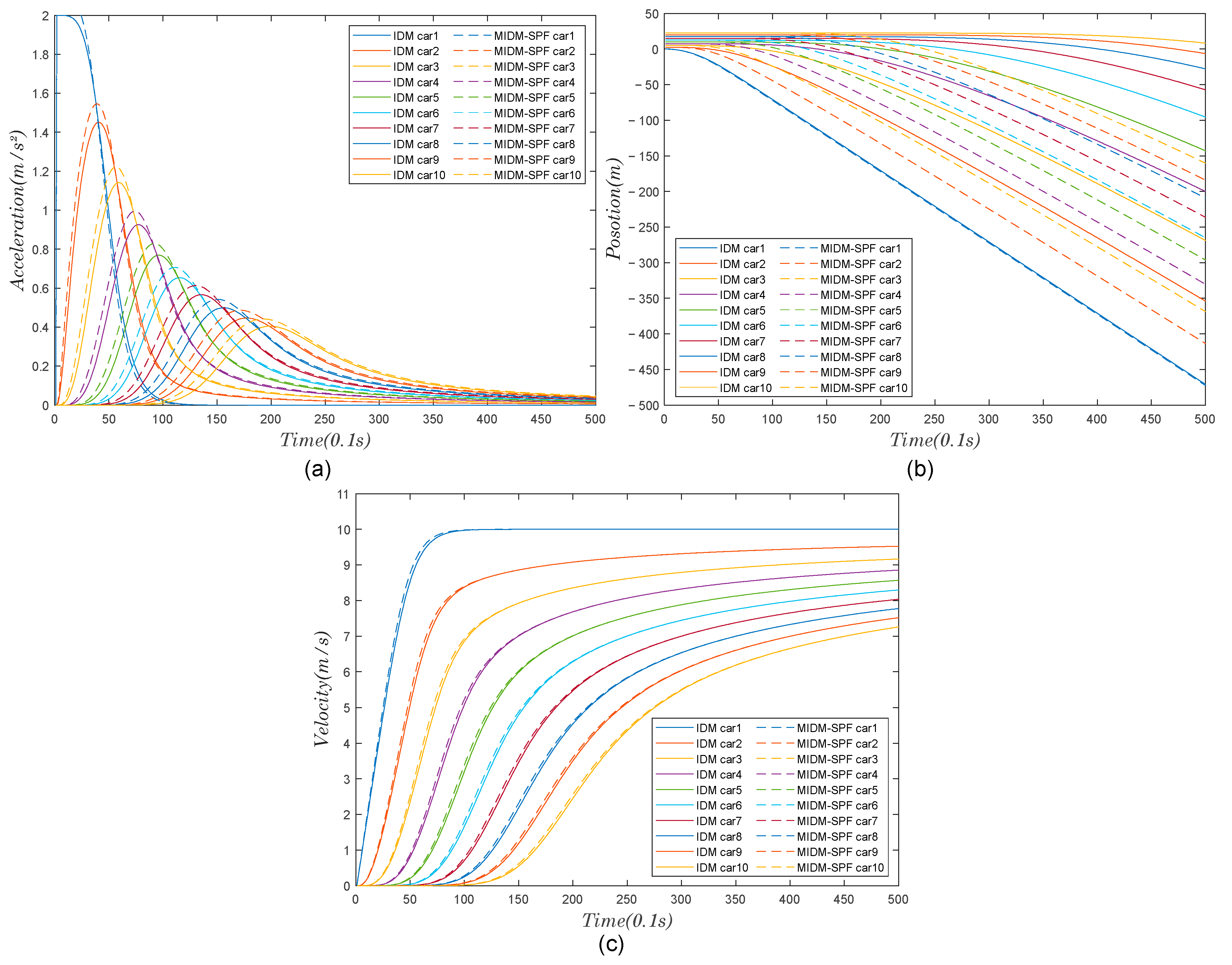
4.2. Dynamic Performance Study of the Model

To examine the dynamic performance of a car-following model involving multiple vehicles with a safety potential field, this study stimulated the movement of a vehicle platoon at a four-way intersection scenario. When the traffic signal was red, all ten vehicles, spaced at 2.5 m apart, remained stationary. At t = 0, as the traffic signal changed from red to green, all vehicles began to accelerate and move, aiming to traverse the intersection swiftly while maintaining stability. The parameter settings for both the MIDM-SPF and IDM are detailed in Table 3, with the time delay td set at 0.15 s and the maximum velocity at 10 m/s.
Figure 6a reveals that the MIDM-SPF model achieves higher acceleration than the IDM at the same moment, reaching its maximum acceleration value in a shorter duration. Figure 6b,c show that the velocity distribution of the MIDM-SPF model attains its maximum value more rapidly within a brief period. This behaviour aligns with real-world driving at intersections, where vehicles typically strive to accelerate to the maximum speed quickly after a traffic signal change, ensuring safety to expedite passing through the intersection. Moreover, compared to the IDM, the MIDM-SPF covers a greater distance within the same amount of time, suggesting that the car-following scenario at the intersection can facilitate more vehicles passing through in a limited time, thereby significantly enhancing the efficiency of vehicle flow at the intersection.
Furthermore, this study created a 400 m circular road scenario to examine the influence of SPFs on traffic flow stability. One hundred vehicles with uniform spacing were tested in this configuration to evaluate their resilience against disturbances and traffic flow oscillations. The sensitivity coefficients, γ and μ, were varied using a controlled variables method for the experiments.
Figure 7a depicts the space headway distribution in the MIDM-SPF model for different γ values (0, 0.1, 0.2, and 0.37) when μ is set to zero in the circular road scenario. Conversely, Figure 7b illustrates the space headway distribution for 100 vehicles in the car-following model when γ is zero and μ varies (0, 0.1, 0.2, and 0.29). With increasing γ and μ, there is a notable decrease in the fluctuation of space headways within the vehicle platoon. This suggests that speed fluctuations caused by initial disturbances in the traffic flow have been effectively absorbed by the system, restoring it to stable traffic conditions. Moreover, as γ and μ change, the incidence of vehicles with varying headways due to disturbances diminishes during the traffic flow stabilisation process. This observation implies that the car-following model with multiple vehicles and a safety potential field effectively mitigates the stop-and-go traffic phenomenon and enhances traffic flow stability.
Figure 8a clearly demonstrates that, under the influence of disturbances, the space–time evolution of traffic flow, with both γ = 0 and μ = 0, is characterised by numerous folding bands. These bands, visible as multiple peaks and valleys on the time–space plane, signify that disturbances are continuously propagating and amplifying within the traffic flow. This leads to an unstable state, potentially manifesting as traffic congestion. In contrast, Figure 8b–d show that as the values of γ and μ incrementally increase, the undulations in the traffic flow’s time–space plot start to decrease, and the folding bands contract. When γ = 0.37 and μ = 0.29, the folding bands almost vanish, and the overall time–space evolution appears significantly flatter. This observation indicates that disturbances within the traffic flow are effectively mitigated, returning the traffic system to a stable state. The MIDM-SPF model is thus shown to effectively absorb disturbances within a car-following scenario, improving overall traffic flow stability.

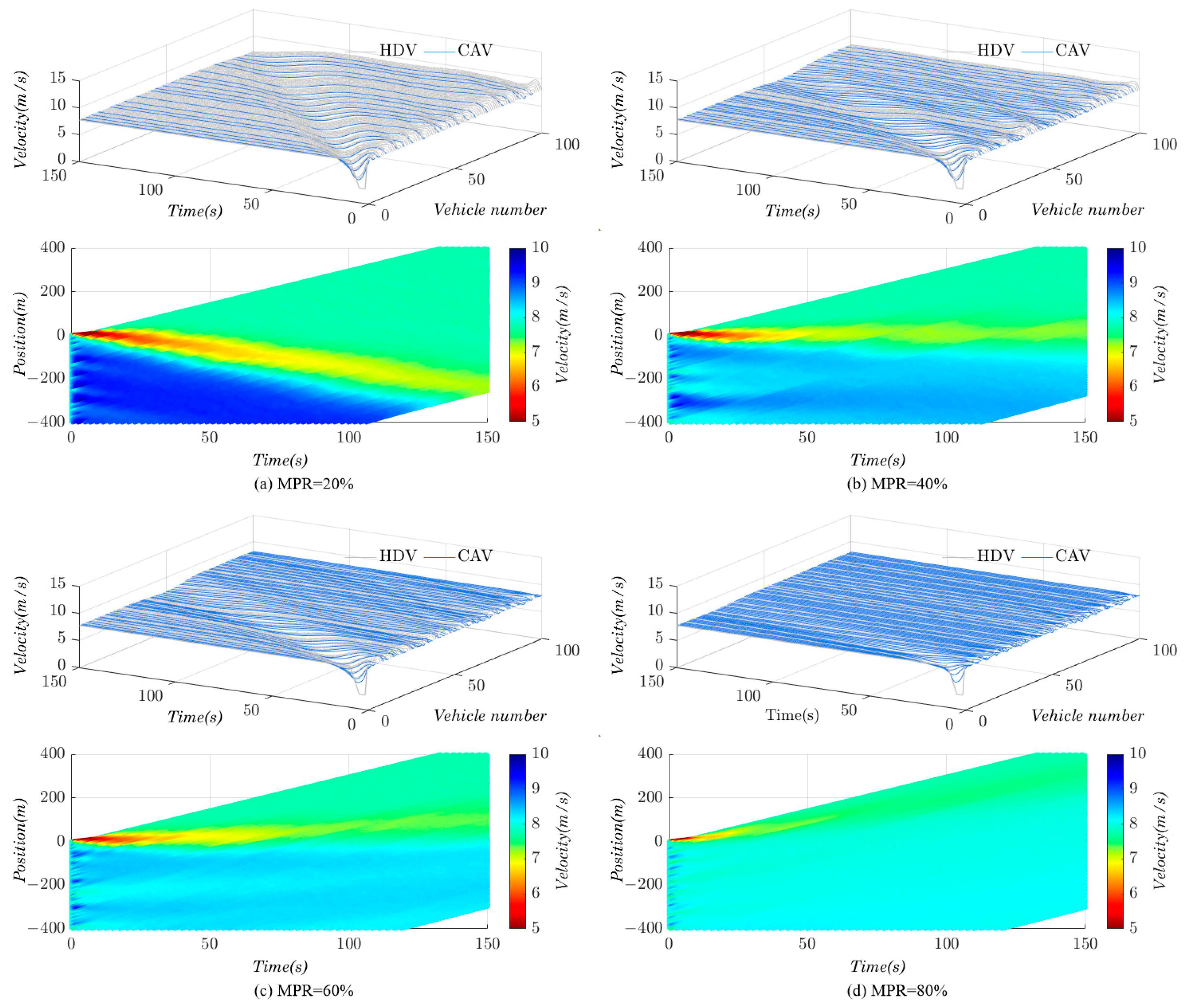
4.3. Simulation Analysis at Different Market Penetration Rates

To further investigate the model’s stability in a mixed traffic flow environment, this study investigates the impact of CAV penetration rates on mixed traffic flow stability. The scenario simulates car-following behaviour in a single-lane mixed traffic flow, focusing on a situation with 100 uniformly distributed vehicles on a road. By varying the proportions of human-driven vehicles (IDM) and CAVs (MIDM-SPF) in the scenario, the study examines the model’s resilience to disturbances in large-scale mixed traffic flows. The initial vehicle speeds were set in the range 7–9 m/s.
Numerical simulations were conducted for CAV market penetration rates (MPRs) of 0.2, 0.4, 0.6, and 0.8. At t = 0, a disturbance was introduced at the leading vehicle’s position to simulate emergency braking behaviour. The resulting velocity and position curves for different MPRs are displayed in Figure 9. In these figures, grey lines represent HDVs, and blue lines represent CAVs. Figure 9a reveals that at a 20% MPR, the disturbance causes significant velocity fluctuations, characterised by an oscillatory behaviour. As the MPR increases, as seen in Figure 9b–d, the extent of velocity fluctuations gradually reduces, the overall speed oscillation trend in the traffic flow diminishes, and the duration of fluctuation decreases. At an 80% MPR, the range of velocity fluctuations and the fluctuation duration are noticeably shorter. These observations suggest that a higher proportion of CAVs in mixed traffic flows can significantly enhance traffic flow stability.

5. Conclusions

This paper proposed a car-following model based on the safety potential field within a connected environment. The stability analysis reveals that the stability region of this model is significantly broader than that of the comparative model. However, incorporating a time delay can modify the motion state of vehicles, thereby impacting traffic flow stability. The experiments indicate that accounting for the SPF of preceding and following vehicles, along with the time delay, enhances traffic flow stability and effectively mitigates congestion. The model parameters were calibrated using real-world data from urban roads, and error analysis was conducted to obtain optimal model parameters. A comparison and analysis of the fitting accuracies of the two models show that the DIDM-SPF provides superior fitting accuracy, indicating its enhanced ability to simulate real traffic flows and offer more reliable predictive and evaluative capabilities. These findings offer valuable insights for optimising traffic flow control and enhancing road traffic efficiency.
Numerical simulations and experimental results indicate that the MIDM-SPF outperforms the IDM in aspects such as vehicle acceleration, speed, and position distribution, aligning more closely with real traffic scenarios. This study also assesses the impact of the MIDM-SPF on the stability of large-scale mixed traffic flow under different MPRs, confirming that the model can effectively stabilise following traffic flow. This model holds significant implications for the development and enhancement of traffic simulation software and algorithms, as well as the design of driving assistance software and platforms. Such advancements can aid drivers in making informed decisions, alleviate traffic congestion, and support the widespread adoption of autonomous driving. Nevertheless, due to the complexity of transportation systems, it is necessary to further expand the calibration samples and conduct more precise parameter calibrations (to verify the model’s performance in different weather conditions or various road types, such as urban roads and rural roads). Moreover, the current model does not address the issue of resource consumption in large-scale deployments, which can also impact the stability of traffic flow. Addressing this issue is an important direction for future research and development.

Author Contributions

Conceptualization, Z.W., W.W., K.M. and S.F.; methodology, Z.W., W.W., K.M. and S.F.; software, Z.W., W.W., K.M. and S.F.; validation, Z.W., W.W., K.M. and S.F.; investigation, Z.W., W.W., K.M. and S.F.; resources, Z.W., W.W., K.M. and S.F.; writing—original draft preparation, Z.W., W.W. and K.M.; writing—review and editing, Z.W., W.W. and S.F.; supervision, Z.W., W.W., K.M. and S.F. All authors have read and agreed to the published version of the manuscript.

Funding

This research was funded by Open Project of Shandong Key Laboratory of Smart Transportation, grant number 2021SDKLST003.

Institutional Review Board Statement

Not applicable.

Informed Consent Statement

Not applicable.

Data Availability Statement

The data presented in this study are available on request from the corresponding author. The data are not publicly available due to privacy.

Acknowledgments

This research was supported by Open Project of Shandong Key Laboratory of Smart Transportation.

Conflicts of Interest

The authors declare no conflicts of interest.

Appendix A

The SPF model, derivation, simulations related to lane markings, road boundaries, and other vehicles are presented in Appendix A.1. The derivation process for the stability analysis of the proposed model can be found in Appendix A.2.

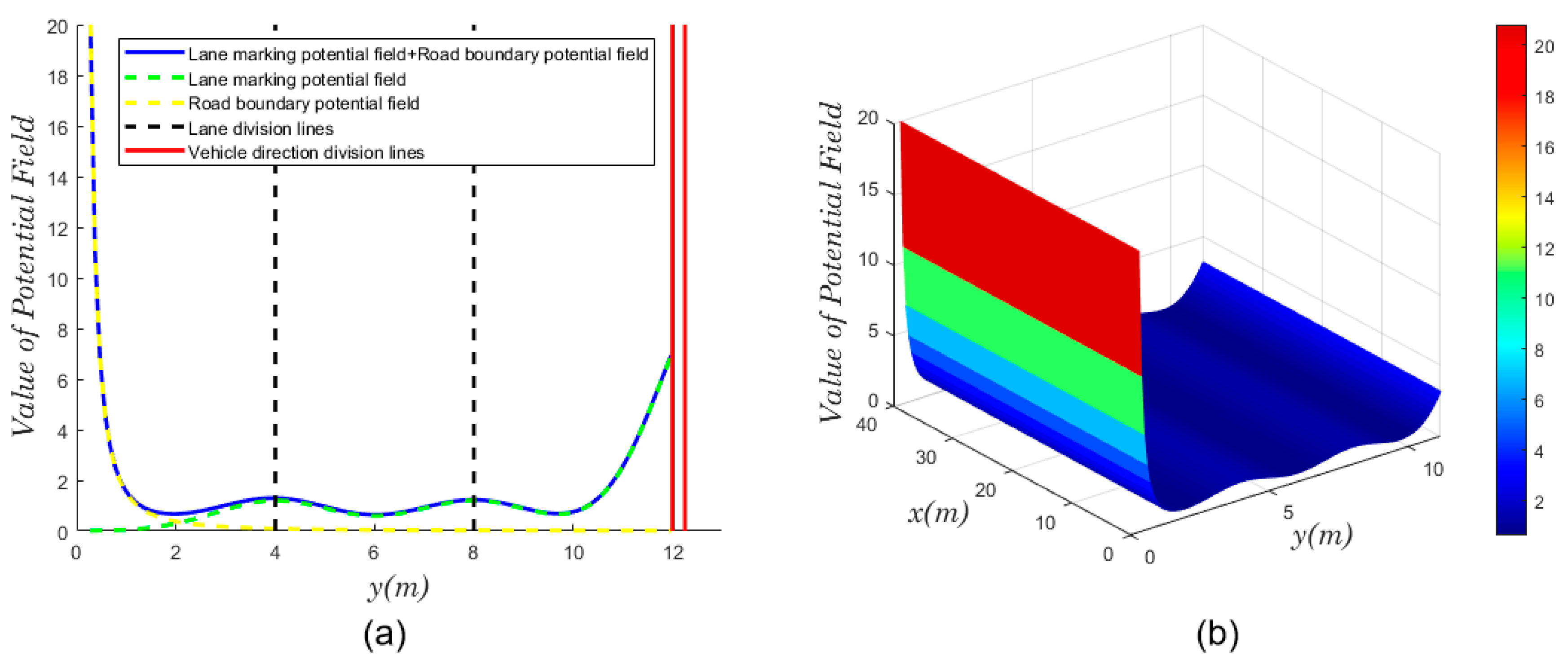
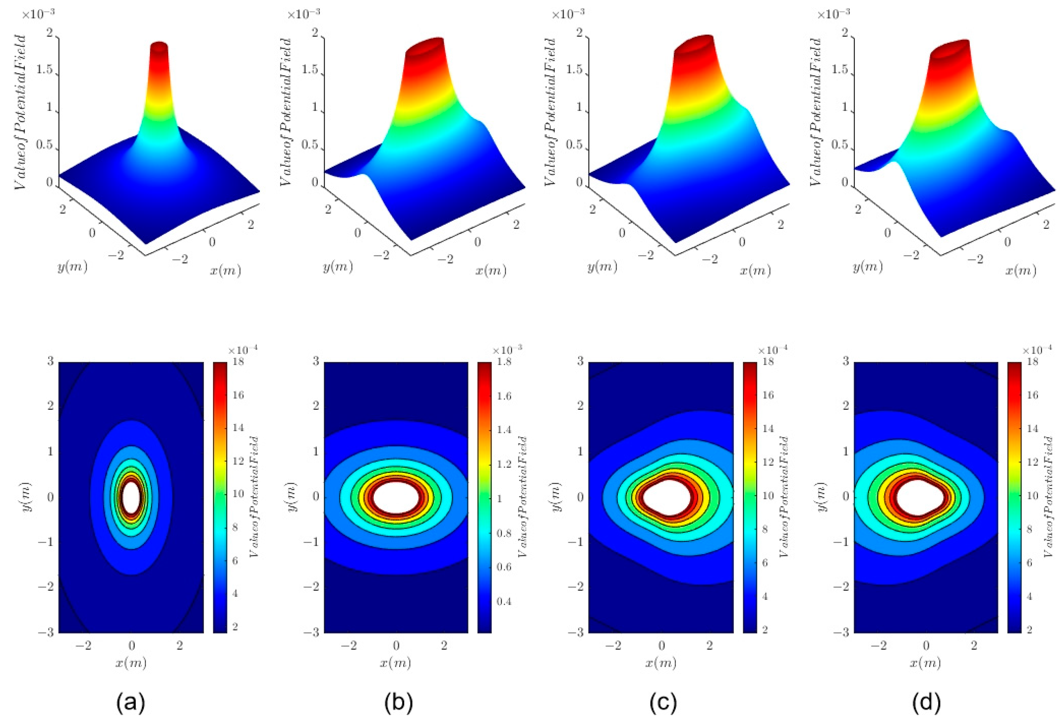
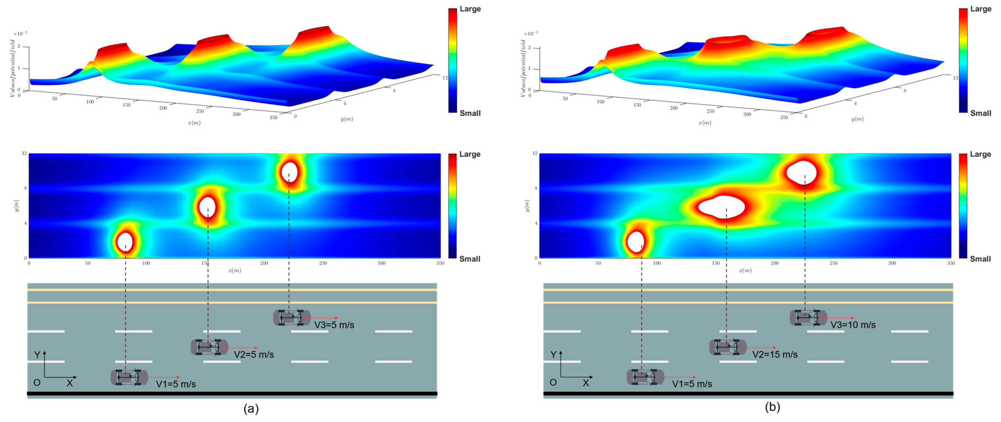
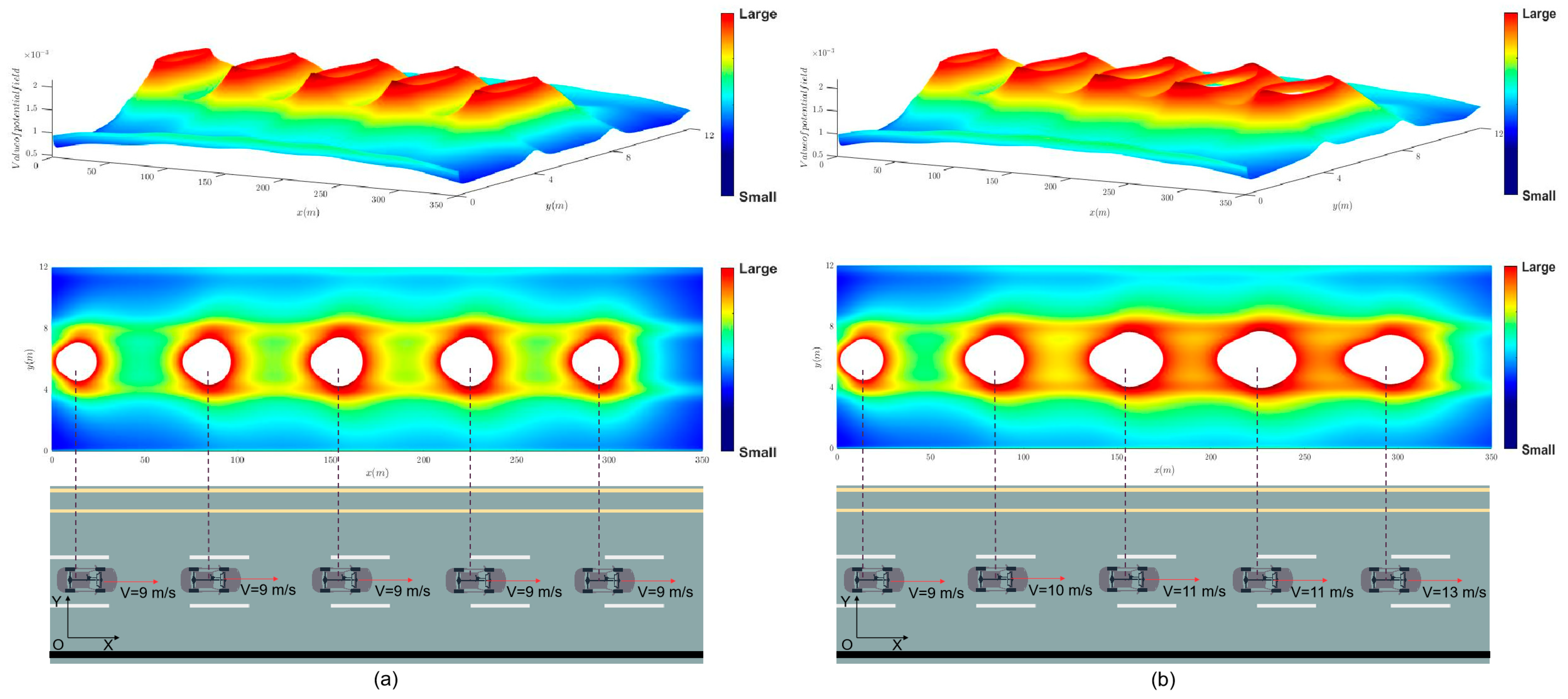
Appendix A.1. Modelling of Safety Potential Field

Lane markings are classified into two types: white lane and yellow vehicle direction division lines (Figure 1). The white lines separate vehicles travelling in the same direction, whereas the yellow lines differentiate vehicles moving in opposite directions. These lane markings impose constraints on vehicle driving, with the safety risk being inversely proportional to the distance from them. The closer a vehicle is to the lane markings, the higher the associated safety risk. Both types of division lines collaboratively restrict the lateral movement of vehicles, aiming to keep vehicles centred in their lanes to the extent possible. The potential field strength of a lane division line is less than that of a vehicle direction division line, as vehicles are permitted to change lanes but must not drive against traffic. The potential field distribution of the lane markings is modelled using a Gaussian function:
U L = i = 1 m L i e y y i 2 2 σ 2 y y i y y i + j = 1 n L j e y y j 2 2 σ 2 y y j y y j ,
where m and n denote the number of lane division lines and vehicle direction division lines, respectively. Li and Lj are the potential field strength coefficients for these lines, related to their peak field strength. y is the lateral coordinate of any point, with yi and yj representing the lateral positions of the lane division and vehicle direction division lines, respectively. σ represents the rate of change in potential field strength, which increases significantly as a vehicle rapidly approaches the road markings.
In contrast to lane markings, the black road boundaries demarcate the maximum range of vehicle movement. Their potential field is more restrictive, tending toward infinity as a vehicle approaches the boundary; this ensures that CAVs remain within the road limits. The function representing the road boundary field is expressed as follows:
U R = k = 1 2 1 2 R k 1 y y k 2 y y k y y k ,
where Rk is the intensity coefficient of the road boundary line’s potential field. yk denotes the transverse coordinate position of the road boundary, with y1 and y2 corresponding to the upper and lower boundaries, respectively. The parameters of both the lane markings and road boundary potential fields are detailed in Table A1.
Table A1. Parameters for lane-marking potential field and road boundary potential field.
ParametersValueParametersValue
L i 1.2 y j = 1 12
L j 10 y j = 2 12.25
σ 1.22 y k = 1 0
y i = 1 4 R k = 1 3
y i = 2 8 R k = 2 3
By integrating the parameters from Table A1 into the models for the lane-marking potential field and the road boundary potential field, the distribution of these potential fields and their combined three-dimensional (3D) representation can be visualised. Figure A1a illustrates this concept: the green dashed line symbolises the potential field of the lane markings, the yellow dashed line represents the potential field of the road boundary, and the blue solid line depicts the cumulative potential field of both. The figure reveals that the peak of the potential field for lane markings is lower than that for the road boundary. The road boundary’s potential field peaks at its actual position in the scene and diminishes substantially as the vehicle distances itself from the boundary. Figure A1b displays a 3D overlay of the potential fields for the two types of lanes. Here, the potential field intensity is minimal at the centre of each lane, indicating that driving in the middle of a lane minimises driving risk. The potential field intensity increases when the vehicle engages in different driving actions or encounters various scene factors.
Figure A1. Distribution of lane-marking potential field and road boundary potential field: (a) the distribution of the potential field; (b) three-dimensional potential field.
Applsci 14 06735 g0a1
The vehicle potential field arises from the vehicle elements within the traffic scenario. The influencing factors include not just the vehicle mass M but also its speed v, acceleration a, positional distance k, and other driving states. In real-world situations, a vehicle approaching a target vehicle from behind faces a significantly higher safety risk than when approaching from the side. Assuming the vehicle’s centre of mass is (x0,y0), the distance k from a point in space to the vehicle is as follows (not accounting for the target vehicle changing lanes and considering s0 as the minimum gap):
k = x x 0 s 0 e v 2 + y y 0 s 0 2 ,
The vehicle potential field model is designed to enable vehicles to respond to the potential fields of nearby vehicles, maintain a safe distance, and adapt their driving strategies based on the potential field distributions. The target vehicle’s potential field impacts surrounding vehicles only within a certain distance. Consequently, this paper constructs a vehicle potential field model that incorporates the vehicle’s own attributes and motion state parameters:
U v = M λ e a cos θ k k k ,
where λ denotes the vehicle potential field strength coefficient, and θ represents the angle between a point x , y around the target vehicle and the spatial coordinates of the vehicle’s centre of mass.
Utilising the vehicle potential field model parameters outlined in Table A2, this study generated 3D potential field and contour projection maps of vehicles under various driving states. Figure A2 graphically represents the potential fields for stationary and uniform motion, as well as acceleration and deceleration phases. In these scenarios, the inner ring of the potential field, centred around the vehicle’s position, tends toward infinity. This suggests that any vehicle entering this inner ring is likely to collide, posing an inevitable safety hazard. Furthermore, the intensity of the potential field progressively decreases with increasing relative distance between vehicles. Figure A2a illustrates a scenario where the target vehicle is stationary, with speed and acceleration zero. Here, the stationary vehicle acts as an obstacle, posing an equal level of risk to other vehicles approaching from any angle. Consequently, the potential field in this scenario assumes a circular shape.
Table A2. Vehicle potential field model parameters.
ParametersValueParametersValue
M k g 1521 s 0 2.6
λ 0.05 x 0 0
θ 0 y 0 0
Figure A2. Distribution of individual vehicle potential fields: (a) v = 0 m/s, a = 0 m/s2; (b) v = 10 m/s, a = 0 m/s2; (c) v = 10 m/s, a = 1.5 m/s2; (d) v = 10 m/s, a = −1.5 m/s2.
Applsci 14 06735 g0a2
Figure A2b depicts a vehicle moving at a constant speed of 10 m/s, with zero acceleration; its motion is aligned along the x-axis. In this case, owing to the absence of velocity along the y-axis, the intensity of the vehicle’s potential field remains unchanged in that direction, irrespective of speed variations. Figure A2c,d illustrate scenarios of acceleration and deceleration at a vehicle speed of 10 m/s, with acceleration rates of 1.5 m/s2 and −1.5 m/s2, respectively. In the acceleration case, the potential field shows a pronounced forward tilt, indicating a greater influence on vehicles ahead of the target vehicle than those behind it. In contrast, in the deceleration scenario, the potential field exhibits a notable backward tilt, implying a lesser impact on vehicles in front compared to those behind the target vehicle.
Figure A3a,b reveal that the intensity of the vehicle potential field increases with the target vehicle’s speed. This suggests that the range of driving risk for other vehicles affected by the target vehicle’s potential field expands at higher rather than at lower speeds. CAVs are capable of obtaining status information about the preceding and following vehicles during transit. By adapting to the actual potential field values of these vehicles, CAVs can maintain, accelerate, or decelerate their speed within safe limits. This capability significantly enhances the stability of vehicle convoys and optimises road capacity for smoother traffic flow.
Figure A3. Distribution of multiple vehicle potential fields for different lanes: (a) same speed (a = 1.5 m/s2); (b) different speed (a = 1.5 m/s2).
Applsci 14 06735 g0a3
The visualisation of the multi-vehicle-following traffic scenario and the vehicle potential field in Figure A4 enables an intuitive assessment of the impact of various traffic factors on driving-safety, with the field strength represented in different colours. A darker colour in this representation indicates a higher level of danger for the vehicle within the traffic environment.
Figure A4. Distribution of multiple vehicle potential fields for car-following scenarios: (a) same speed (a = 1.5 m/s2); (b) different speed (a = 1.5 m/s2).
Applsci 14 06735 g0a4

Appendix A.2. Stability Analysis of the Proposed Model

Linearising (14), we obtain
y n t + t d = f n s y n 1 t y n t + f n v n y n t + f n Δ v y n t y n 1 t + f n a n i y n i t + f n a n + j y n + j t + f n v n i y n i t + f n v n + j y n + j t + f n Δ x i y n i t y n t + f n Δ x j y n + j t y n t , ,
where f n s = f n s v ¯ , s ¯ 0 , f n v n = f n v n v ¯ , s ¯ 0 , f n Δ v = f n Δ v v ¯ , s ¯ 0 , f n a n i = f n a n i v ¯ , s ¯ 0 , f n a n + j = f n a n + j v ¯ , s ¯ 0 , f n v n i = f n v n i v ¯ , s ¯ 0 , f n v n + j = f n v n + j v ¯ , s ¯ 0 , f n Δ x i = f n s v ¯ , s ¯ 0 and f n Δ x j = f n s v ¯ , s ¯ 0 .
We then rewrite (A5) to obtain the difference equation:
y n t + 2 t d y n t + t d = t d f n s y n 1 t y n t + f n v n y n t + t d y n t + f n Δ v y n t + t d y n t y n 1 t + t d + y n 1 t + f n a n i y n i t + t d y n i t + f n a n + j y n + j t + t d y n + j t + f n v n i y n i t + t d y n i t + f n v n + j y n + j t + t d y n + j t +   t d f n Δ x i y n i t y n t + t d f n Δ x j y n + j t y n t ,
Substituting y n t = c e ω α k n + z t and y n t = z c e ω α k n + z t into (A6) and simplifying, we obtain:
e z t d 1 [ z e z t d f n v n f n Δ v 1 e ω α k z f n a n i + f n v n i e i ω α k z f n a n + j + f n v n + j e j ω α k ] = t d [ f n s e ω α k 1 + f n Δ x i e i ω α k 1 + f n Δ x j e j ω α k 1 ] ,
We then expand the power series for the parameters in (A7).
z = z 1 ω α k + z 2 ω α k 2 + ,
e z t d = 1 + t d z + t d 2 z 2 2 + ,
e ω α k = 1 ω α k + ω α k 2 2 ,
Expanding this gives the first- and second-order expressions for z:
z 1 ω α k + z 2 ω α k 2 + t d 2 z 1 ω α k + z 2 ω α k 2 2 × z 1 ω α k + z 2 ω α k 2 + t d z 1 ω α k + z 2 ω α k 2 2 + t d 2 2 z 1 ω α k + z 2 ω α k 2 3 f n v n f n Δ v ω α k ω α k 2 2 z 1 ω α k + z 2 ω α k 2 f n a n i + f n v n i 1 i ω α k + i 2 2 ω α k 2 z 1 ω α k + z 2 ω α k 2 f n a n + j + f n v n + j 1 + j ω α k + j 2 2 ω α k 2 = f n s i f n Δ x i + j f n Δ x j ω α k + 1 2 f n s + i 2 2 f n Δ x i + j 2 2 f n Δ x j ω α k 2 ,
and thus yields:
z 1 = f n s + i f n Δ x i j f n Δ x j f n v n + f n v n i + f n v n + j ,
z 2 = z 1 2 1 f n a n i f n a n + j t d 2 f n v n t d 2 f n v n i t d 2 f n v n + j z 1 f n Δ v i f n v n i + j f n v n + j 1 2 f n s + i 2 2 f n Δ x i + j 2 2 f n Δ x j × 1 f n v n + f n v n i + f n v n + j ,
Traffic flows become unstable when z 2 < 0 in response to small perturbations and stabilise when z 2 > 0 . The stability conditions are
f n s + i f n Δ x i j f n Δ x j f n v n + f n v n i + f n v n + j 2 1 f n a n i f n a n + j t d 2 f n v n t d 2 f n v n i t d 2 f n v n + j f n s + i f n Δ x i j f n Δ x j f n v n + f n v n i + f n v n + j f n Δ v i f n v n i + j f n v n + j 1 2 f n s + i 2 2 f n Δ x i + j 2 2 f n Δ x j < 0 ,
Simplifying and rearranging the terms yields:
t d 2 < 1 f n a n i f n a n + j f n v n + f n v n i + f n v n + j + f n Δ v i f n v n i + j f n v n + j f n s + i f n Δ x i j f n Δ x j + f n v n + f n v n i + f n v n + j f n s + i 2 f n Δ x i + j 2 f n Δ x j 2 f n s + i f n Δ x i j f n Δ x j 2 ,
The expressions for f n s , f n v n , f n Δ v , f n a n i , f n a n + j , f n v n i , f n v n + j , f n Δ x i and f n Δ x j can be obtained from (8) as follows:
f n s = 2 a 0 s n t s 0 + T v n t + v n t Δ v t 2 a 0 b s n t 2 ,
f n v n = 2 a 0 2 v 0 v n t v 0 3 + T + Δ v 2 a 0 b s 0 + T v n t + v n t Δ v 2 a 0 b s n 2 t γ i = 1 p M n i λ e a n i + v n i x i · s 0 e v n μ j = 1 q M n + j λ e a n + j + v n + j x j · s 0 e v n ,
f n Δ v = s 0 + T v n t + v n t Δ v 2 a 0 b v n t s n 2 t a 0 b ,
f n a n i = γ i = 1 p 1 + M n i λ e v n + v n i x i · s 0 e a n i ,
f n a n + j = μ j = 1 q 1 + M n + j λ e v n + v n + j x j · s 0 e a n + j ,
f n v n i = γ i = 1 p M n i λ e a n i + v n x i · s 0 e v n i ,
f n v n + j = = μ j = 1 q M n + j λ e a n i + v n x j · s 0 e v n + j ,
f n Δ x i = γ i = 1 p M n i λ e a n i + v n i S 0 Δ x i 2 e v n ,
f n Δ x j = μ j = 1 q M n + j λ e a n + j + v n + j S 0 Δ x j 2 e v n ,
By substituting (A16)–(A24) into (A15), the stability condition is
t d 2 < 0.5 · 1 γ i = 1 p 1 + M n i λ e v n + v n i x i · s 0 e a n i μ j = 1 q 1 + M n + j λ e v n + v n + j x j · s 0 e a n + j a 0 2 v 0 v n t v 0 3 + T s 0 + T v n t s n 2 t + γ i = 1 p M n i λ e a n i + v n i x i · s 0 e v n + μ j = 1 q M n + j λ e a n + j + v n + j x j · s 0 e v n + s 0 + T v n t v n t s n 2 t a 0 b + i γ i = 1 p M n i λ e a n i + v n x i · s 0 e v n i j μ j = 1 q M n + j λ e a n i + v n x j · s 0 e v n + j 2 a 0 s n t s 0 + T v n t s n t 2 + i γ i = 1 p M n i λ e a n i + v n i S 0 Δ x i 2 e v n j μ j = 1 q M n + j λ e a n + j + v n + j S 0 Δ x j 2 e v n + a 0 2 v 0 v n t v 0 3 + T s 0 + T v n t s n 2 t + γ i = 1 p M n i λ e a n i + v n i x i · s 0 e v n + μ j = 1 q M n + j λ e a n + j + v n + j x j · s 0 e v n × 2 a 0 s n t s 0 + T v n t s n t 2 + i 2 γ i = 1 p γ i = 1 p M n i λ e a n i + v n i S 0 Δ x i 2 e v n + j 2 μ j = 1 q M n + j λ e a n + j + v n + j S 0 Δ x j 2 e v n 2 a 0 s n t s 0 + T v n t s n t 2 + i γ γ i = 1 p M n i λ e a n i + v n i S 0 Δ x i 2 e v n j μ j = 1 q M n + j λ e a n + j + v n + j S 0 Δ x j 2 e v n 2 ,

References

  1. Khatib, O. Real-time obstacle avoidance for manipulators and mobile robots. Int. J. Robot. Res. 1986, 5, 90–98. [Google Scholar] [CrossRef]
  2. Yi, Z.; Li, L.; Qu, X.; Hong, Y.; Mao, P.; Ran, B. Using artificial potential field theory for a cooperative control model in a connected and automated vehicles environment. Transp. Res. Rec. 2020, 2674, 1005–1018. [Google Scholar] [CrossRef]
  3. Wang, R.; Guo, J.; Guo, S.; Fu, Q.; Xu, J. Cooperative hunting of spherical multi-robots based on improved artificial potential field method. In Proceedings of the 2022 IEEE International Conference on Mechatronics and Automation (ICMA), Guilin, China, 7–10 August 2022; pp. 575–580. [Google Scholar] [CrossRef]
  4. Wang, B.; Zhou, K.; Qu, J. Research on multi-robot local path planning based on improved artificial potential field method. In Proceedings of the Fifth Euro-China Conference on Intelligent Data Analysis and Applications 5, Xi’an, China, 12–14 October 2018; Springer International Publishing: Berlin/Heidelberg, Germany, 2019; pp. 684–690. [Google Scholar]
  5. Shi, M.; Nie, J. Improvement of Path Planning Algorithm based on Small Step Artificial Potential Field Method. In Proceedings of the 2022 9th International Conference on Dependable Systems and Their Applications (DSA), Ürümqi, China, 4–5 August 2022; pp. 827–831. [Google Scholar] [CrossRef]
  6. Liu, Y.; Wang, T.; Xu, H. PE-A* Algorithm for Ship Route Planning Based on Field Theory. IEEE Access 2022, 10, 36490–36504. [Google Scholar] [CrossRef]
  7. Zhai, L.; Feng, S. An improved ant colony algorithm based on artificial potential field and quantum evolution theory. J. Intell. Fuzzy Syst. 2022, 42, 5773–5788. [Google Scholar] [CrossRef]
  8. Li, Y.; Yu, B.; Chen, Y.; Hu, Z. A new theory of driver vision pressure energy field and its application in driver behaviour decision-making model. IET Intell. Transp. Syst. 2022, 16, 1–12. [Google Scholar] [CrossRef]
  9. Semsar-Kazerooni, E.; Verhaegh, J.; Ploeg, J.; Alirezaei, M. Cooperative adaptive cruise control: An artificial potential field approach. In Proceedings of the 2016 IEEE Intelligent Vehicles Symposium (IV), Gothenburg, Sweden, 19–22 June 2016; pp. 361–367. [Google Scholar] [CrossRef]
  10. Liu, W.; Li, Z. Comprehensive predictive control method for automated vehicles in dynamic traffic circumstances. IET Intell. Transp. Syst. 2018, 12, 1455–1463. [Google Scholar] [CrossRef]
  11. Xu, Y.; Ma, Z.; Sun, J. Simulation of turning vehicles’ behaviors at mixed-flow intersections based on potential field theory. Transp. B Transp. Dyn. 2018, 7, 498–518. [Google Scholar] [CrossRef]
  12. Ma, Y.; Zhang, P.; Hu, B. Active lane-changing model of vehicle in B-type weaving region based on potential energy field theory. Phys. A Stat. Mech. Its Appl. 2019, 535, 122291. [Google Scholar] [CrossRef]
  13. Joo, Y.J.; Kim, E.J.; Kim, D.K.; Park, P.Y. A generalized driving risk assessment on high-speed highways using field theory. Anal. Methods Accid. Res. 2023, 40, 100303. [Google Scholar] [CrossRef]
  14. Cheng, Y.; Liu, Z.; Gao, L.; Zhao, Y.; Gao, T. Traffic risk environment impact analysis and complexity assessment of autonomous vehicles based on the potential field method. Int. J. Environ. Res. Public Health 2022, 19, 10337. [Google Scholar] [CrossRef]
  15. Zhao, H.; He, R.; Ma, C. An extended car-following model at signalised intersections. J. Adv. Transp. 2018, 2018, 5427507. [Google Scholar] [CrossRef]
  16. Gazis, D.C.; Herman, R.; Rothery, R.W. Nonlinear follow-the-leader models of traffic flow. Oper. Res. 1961, 9, 545–567. [Google Scholar] [CrossRef]
  17. Kometani, E. Dynamic behavior of traffic with a nonlinear spacing-speed relationship. Theory Traffic Flow (Proc. Sym. TTF (GM)) 1959, 105–119. [Google Scholar]
  18. Michaels, R.M. Perceptual Factors in Car Following. In Proceedings of the Second International Symposium on the Theory of Traffic Flow, London, UK, 25–27 June 1963; pp. 44–59. [Google Scholar]
  19. Kikuchi, S.; Chakroborty, P. Car-following model based on fuzzy inference system. Transp. Res. Rec. 1992, 1194, 82. [Google Scholar]
  20. Bando, M.; Hasebe, K.; Nakayama, A.; Shibata, A.; Sugiyama, Y. Dynamical model of traffic congestion and numerical simulation. Phys. Rev. E 1995, 51, 1035. [Google Scholar] [CrossRef] [PubMed]
  21. Wang, L.; Wang, B.H.; Hu, B. Cellular automaton traffic flow model between the Fukui-Ishibashi and Nagel-Schreckenberg models. Phys. Rev. E 2001, 63, 056117. [Google Scholar] [CrossRef]
  22. Yang, Z.S.; Yu, Y.; Yu, D.X.; Zhou, H.X.; Mo, X.L. APF-based car following behavior considering lateral distance. Adv. Mech. Eng. 2013, 5, 207104. [Google Scholar] [CrossRef]
  23. Li, C.; Jiang, X.; Wang, W.; Cheng, Q.; Shen, Y. A simplified car-following model based on the artificial potential field. Procedia Eng. 2016, 137, 13–20. [Google Scholar] [CrossRef]
  24. Jia, Y.; Qu, D.; Han, L.; Lin, L.; Hong, J. Research on car-following model based on molecular dynamics. Adv. Mech. Eng. 2021, 13, 1687814021993003. [Google Scholar] [CrossRef]
  25. Zhang, G.; Yin, S.; Huang, C.; Zhang, W. Intervehicle Security-Based Robust Neural Formation Control for Multiple USVs via APS Guidance. J. Mar. Sci. Eng. 2023, 11, 1020. [Google Scholar] [CrossRef]
  26. Shen, C.; Xiao, X.; Su, W.; Tong, Y.; Hu, H. Research on V2V time headway strategy considering multi-front vehicles based on artificial potential field. Electronics 2023, 12, 3602. [Google Scholar] [CrossRef]
  27. Wang, J.; Wu, J.; Li, Y.; Li, K. The concept and modeling of driving safety field based on driver-vehicle-road interactions. In Proceedings of the 17th International IEEE Conference on Intelligent Transportation Systems (ITSC), Qingdao, China, 8–11 October 2014; pp. 974–981. [Google Scholar] [CrossRef]
  28. Wang, J.; Wu, J.; Li, Y. The driving safety field based on driver–vehicle–road interactions. IEEE Trans. Intell. Transp. Syst. 2015, 16, 2203–2214. [Google Scholar] [CrossRef]
  29. Wang, J.; Wu, J.; Zheng, X.; Ni, D.; Li, K. Driving safety field theory modeling and its application in pre-collision warning system. Transp. Res. Part C Emerg. Technol. 2016, 72, 306–324. [Google Scholar] [CrossRef]
  30. Li, M.; Song, X.; Cao, H.; Wang, J.; Huang, Y.; Hu, C.; Wang, H. Shared control with a novel dynamic authority allocation strategy based on game theory and driving safety field. Mech. Syst. Signal Process. 2019, 124, 199–216. [Google Scholar] [CrossRef]
  31. Li, L.; Gan, J.; Yi, Z.; Qu, X.; Ran, B. Risk perception and the warning strategy based on safety potential field theory. Accid. Anal. Prev. 2020, 148, 105805. [Google Scholar] [CrossRef]
  32. Li, L.; Gan, J.; Zhou, K.; Qu, X.; Ran, B. A novel lane-changing model of connected and automated vehicles: Using the safety potential field theory. Phys. A Stat. Mech. Its Appl. 2020, 559, 125039. [Google Scholar] [CrossRef]
  33. Li, L.; Ji, X.; Gan, J.; Qu, X.; Ran, B. A macroscopic model of heterogeneous traffic flow based on the safety potential field theory. IEEE Access 2021, 9, 7460–7470. [Google Scholar] [CrossRef]
  34. Talal, M.; Ramli, K.N.; Zaidan, A.A.; Zaidan, B.B.; Jumaa, F. Review on car-following sensor based and data-generation mapping for safety and traffic management and road map toward ITS. Veh. Commun. 2020, 25, 100280. [Google Scholar] [CrossRef]
  35. Li, L.; Gan, J.; Ji, X.; Qu, X.; Ran, B. Dynamic driving risk potential field model under the connected and automated vehicles environment and its application in car-following modeling. IEEE Trans. Intell. Transp. Syst. 2020, 23, 122–141. [Google Scholar] [CrossRef]
  36. Li, L.; Gan, J.; Qu, X.; Mao, P.; Yi, Z.; Ran, B. A novel graph and safety potential field theory-based vehicle platoon formation and optimization method. Appl. Sci. 2021, 11, 958. [Google Scholar] [CrossRef]
  37. Wu, R.; Li, L.; Shi, H.; Rui, Y.; Ngoduy, D.; Ran, B. A Driving Risk Surrogate and Its Application in Car-Following Scenario at Expressway. arXiv 2022, arXiv:2211.03304. [Google Scholar]
  38. Jia, Y.; Qu, D.; Song, H.; Wang, T.; Zhao, Z. Car-following characteristics and model of connected autonomous vehicles based on safe potential field. Phys. A Stat. Mech. Its Appl. 2022, 586, 126502. [Google Scholar] [CrossRef]
  39. Li, L.; Wang, C.; Zhang, Y.; Qu, X.; Li, R.; Chen, Z.; Ran, B. Microscopic state evolution model of mixed traffic flow based on potential field theory. Phys. A Stat. Mech. Its Appl. 2022, 607, 128185. [Google Scholar] [CrossRef]
  40. Ma, Y.; Dong, F.; Yin, B.; Lou, Y. Real-time risk assessment model for multi-vehicle interaction of connected and autonomous vehicles in weaving area based on risk potential field. Phys. A Stat. Mech. Its Appl. 2023, 620, 128725. [Google Scholar] [CrossRef]
  41. Menzel, T.; Bagschik, G.; Isensee, L.; Schomburg, A.; Maurer, M. From functional to logical scenarios: Detailing a keyword-based scenario description for execution in a simulation environment. In Proceedings of the 2019 IEEE Intelligent Vehicles Symposium (IV), Paris, France, 9–12 June 2019; pp. 2383–2390. [Google Scholar] [CrossRef]
  42. Treiber, M.; Hennecke, A.; Helbing, D. Congested traffic states in empirical observations and microscopic simulations. Phys. Rev. E 2020, 62, 1805. [Google Scholar] [CrossRef] [PubMed]
  43. Treiber, M.; Kesting, A. The intelligent driver model with stochasticity-new insights into traffic flow oscillations. Transp. Res. Procedia 2017, 23, 174–187. [Google Scholar] [CrossRef]
  44. Zhao, H.; Chen, Q.; Shi, W.; Gu, T.; Li, W. Stability analysis of an improved car-following model accounting for the driver’s characteristics and automation. Phys. A Stat. Mech. Its Appl. 2019, 526, 120990. [Google Scholar] [CrossRef]
  45. Wang, Y.; Li, X.; Tian, J.; Jiang, R. Stability analysis of stochastic linear car-following models. Transp. Sci. 2020, 54, 274–297. [Google Scholar] [CrossRef]
  46. Wang, X.; Liu, M.; Ci, Y.; Wu, L. Effect of front two adjacent vehicles’ velocity information on car-following model construction and stability analysis. Phys. A Stat. Mech. Its Appl. 2022, 607, 128196. [Google Scholar] [CrossRef]
  47. Li, Y.; Chen, B.; Zhao, H.; Peeta, S.; Hu, S.; Wang, Y.; Zheng, Z. A car-following model for connected and automated vehicles with heterogeneous time delays under fixed and switching communication topologies. IEEE Trans. Intell. Transp. Syst. 2021, 23, 14846–14858. [Google Scholar] [CrossRef]
  48. Abualigah, L.; Diabat, A.; Mirjalili, S.; Abd Elaziz, M.; Gandomi, A.H. The arithmetic optimization algorithm. Comput. Methods Appl. Mech. Eng. 2021, 376, 113609. [Google Scholar] [CrossRef]
  49. Gölcük, İ.; Ozsoydan, F.B.; Durmaz, E.D. An improved arithmetic optimization algorithm for training feedforward neural networks under dynamic environments. Knowl.-Based Syst. 2023, 263, 110274. [Google Scholar] [CrossRef]
  50. Kathiravan, K.; Rajnarayanan, P.N. Application of AOA algorithm for optimal placement of electric vehicle charging station to minimize line losses. Electr. Power Syst. Res. 2023, 214, 108868. [Google Scholar] [CrossRef]
  51. Çelik, E. IEGQO-AOA: Information-exchanged gaussian arithmetic optimization algorithm with quasi-opposition learning. Knowl.-Based Syst. 2023, 260, 110169. [Google Scholar] [CrossRef]
Figure 1. Traffic scenarios based on SPF: (a) scenario building; (b) description of scenario elements.
Applsci 14 06735 g001
Figure 2. Schematic multi-vehicle car-following model.
Applsci 14 06735 g002
Figure 3. Stability curves for different γ and μ : (a) td = 0 (b) td = 0.15.
Applsci 14 06735 g003
Figure 4. Comparison of convergence curves of different functions: (a) F1; (b) F2; (c) F10; (d) F11.
Applsci 14 06735 g004
Figure 5. Front and rear vehicle fitted trajectory data curves: (a) front vehicle; (b) rear vehicle.
Applsci 14 06735 g005
Figure 6. Vehicle speed, position, and acceleration distribution curves: (a) acceleration; (b) position; (c) velocity.
Applsci 14 06735 g006
Figure 7. Comparison of the different space headways of different γ and μ: (a) different γ ; (b) different μ.
Applsci 14 06735 g007
Figure 8. Time–space evolution of velocity with different γ μ: (a) γ = 0 , μ = 0; (b) γ = 0.1 , μ = 0; (c) γ = 0 , μ = 0; (d) γ = 0.37 , μ = 0.29.
Applsci 14 06735 g008
Figure 9. Spatial–temporal trajectories obtained at different MPRs: (a) MPR = 20% (b) MPR = 40% (c) MPR = 60% (d) MPR = 80%.
Applsci 14 06735 g009
Table 1. Overview of the car-following behaviour modelling works related to SPF.
AuthorsInformation from Multiple VehiclesTime DelayStability AnalysisCalibration of Relevant ParametersMixed Traffic
Li et al. [35]XXX X
Li et al. [36] XXXX
Wu et al. [37]XXX X
Jia et al. [38] XX X
Li et al. [39]XXXX
Ma et al. [40] XX
This study
Table 2. Benchmark functions.
NameFunctionRangeDimension
F1 i = 1 n x i 2 [−100, 100]30
F2 i = 1 n x i + i = 1 n x i [−10, 10]30
F10 20 e x p ( 0.2 1 n i = 1 n x i 2 ) e x p ( i = 1 n c o s ( 2 π x i ) ) + 20 + e [−32, 32] 30
F11 1 4000 i = 1 n x i 2 i = 1 n c o s ( x i i ) + 1 [−600, 600] 30
Table 3. Calibration results of MIDM-SPF model parameters.
ParametersDescriptionBoundariesValue
a0Maximum acceleration[0.1,5]2.2
bComfortable deceleration[0.1,5]1.4
s0Minimum headway[0.1,10]3.6
TSafe time headway[0.1,5]1.5
λvehicle potential field strength coefficient[0.1,1]0.11
γ The coefficient of the safety potential field for the leading vehicle[0.1,1]0.37
μ The coefficient of the safety potential field for the following vehicle[0.1,1] 0.29
Table 4. Fitting error data corresponding to the two models.
ModelMEMAERMSER2
IDM0.1920.2790.38395.6%
MIDM-SPF0.1030.2490.35197.9%
Disclaimer/Publisher’s Note: The statements, opinions and data contained in all publications are solely those of the individual author(s) and contributor(s) and not of MDPI and/or the editor(s). MDPI and/or the editor(s) disclaim responsibility for any injury to people or property resulting from any ideas, methods, instructions or products referred to in the content.

