Optimizing Recurrent Neural Networks: A Study on Gradient Normalization of Weights for Enhanced Training Efficiency

Abstract

Recurrent Neural Networks (RNNs) are classical models for processing sequential data, demonstrating excellent performance in tasks such as natural language processing and time series prediction. However, during the training of RNNs, the issues of vanishing and exploding gradients often arise, significantly impacting the model’s performance and efficiency. In this paper, we investigate why RNNs are more prone to gradient problems compared to other common sequential networks. To address this issue and enhance network performance, we propose a method for gradient normalization of network weights. This method suppresses the occurrence of gradient problems by altering the statistical properties of RNN weights, thereby improving training effectiveness. Additionally, we analyze the impact of weight gradient normalization on the probability-distribution characteristics of model weights and validate the sensitivity of this method to hyperparameters such as learning rate. The experimental results demonstrate that gradient normalization enhances the stability of model training and reduces the frequency of gradient issues. On the Penn Treebank dataset, this method achieves a perplexity level of 110.89, representing an 11.48% improvement over conventional gradient descent methods. For prediction lengths of 24 and 96 on the ETTm1 dataset, Mean Absolute Error (MAE) values of 0.778 and 0.592 are attained, respectively, resulting in 3.00% and 6.77% improvement over conventional gradient descent methods. Moreover, selected subsets of the UCR dataset show an increase in accuracy ranging from 0.4% to 6.0%. The gradient normalization method enhances the ability of RNNs to learn from sequential and causal data, thereby holding significant implications for optimizing the training effectiveness of RNN-based models.

1. Introduction

Recurrent Neural Networks (RNNs) are characterized by periodic memory capacity and thus are able to retain previous information while processing sequential data, and they are widely used in the fields of natural language processing [1], speech recognition [2], image description [3], video analytics [4], and so on.

Despite the emergence of various improved RNN models like LSTM and GRU, after years of research, their core structure remains recurrent. That is, at each time step, they utilize the current input along with the hidden state from the previous time step to compute the output and the hidden state for the next time step. However, it is this recurrent structure that primarily makes RNN models more susceptible to issues such as vanishing and exploding gradients compared to feedforward models.

The causes of gradient problems can generally be divided into two categories. One is the gradient cumulative product hypothesis [5], and the other is the neuron saturation hypothesis [6]. The former suggests that gradient disappearance and explosion mainly occur because, during the backward propagation process of model training, the gradient of weights is calculated progressively through the “chain rule”. As the depth of the neural network increases, the gradients of weights closer to the bottom layer become increasingly smaller or larger. If the gradient is too small, it is referred to as a vanishing gradient; if it is too large, it is called an exploding gradient. The latter suggests that the cause of gradient problems lies in the nonlinearity of neuron functions and the existence of activation and inhibition zones. This hypothesis suggests that common neuron functions, such as Sigmoid [7], Tanh [8], or ReLU [9], have gradients that are nonlinear. For instance, the gradients of the Sigmoid and Tanh functions are small when the absolute value of the input is greater than 1, leading to non-activation, while ReLU is non-activated in the negative domain. A large number of neurons entering the non-activation zone in the neural network will cause the model to lose its learning ability, ultimately resulting in the failure of model training to converge.

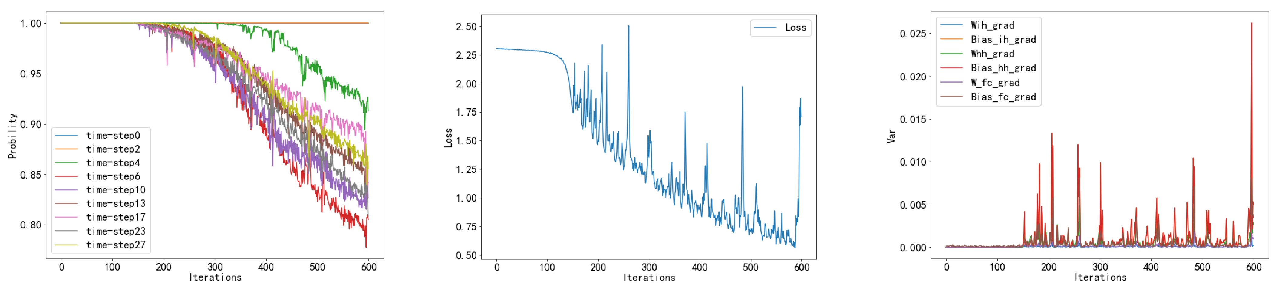
The mechanism behind the gradient problems in RNN models is explored in this article. Firstly, we find that during the model training process, rapid changes in statistical variables of weight gradients such as mean and variance often lead to a large number of activations of the model’s activation functions entering the inhibition zone. At the same time, the recurrent structure characteristic of RNN models implies that the hidden layer weights are reused across the time-step dimension, leading to resonance in the variation of statistical weight properties across the time-step dimension. During training, almost synchronous occurrences of gradient explosions and disappearances happen at different time steps (as shown in Figure 1), and there is a significant synchronous effect between the sudden increase in weight gradient variance, a sudden increase in loss value, and a large number of neurons entering the inhibition zone. To suppress gradient problems, we propose a weight gradient normalization method (WGN) that optimizes the statistical parameters of weights such as mean, variance, etc., during the model training process, avoiding abrupt changes in weight distribution characteristics. Through the analysis and derivation of parameters such as covariance between weight initial values and gradients, covariance between weight gradients, learning rate, etc., we demonstrate that the method is effective in ensuring that the mean of the weights and the rate of change of the variance are stable. In experiments, we apply the weight gradient normalization method to LSTM [10] and Simple-RNN models and validate its effectiveness on the MINIST [11], PTB [12], ETTm1 [13], and UCR [14] datasets. Finally, we discuss the applicability and scalability of this method.

The innovation of this paper is as follows:

• From the perspective of the variance and covariance of weight gradients, the phenomenon of gradient explosion and disappearance in recurrent neural networks is explored, to some extent explaining the causes of gradient problems.
• Based on statistics, a weight gradient normalization method is proposed, which can effectively accelerate the training speed while suppressing gradient explosion and disappearance during the training process.
• A quantification method for the degree of gradient anomaly is proposed, providing a basis for evaluating the effectiveness of gradient problem suppression methods.

2. Related Work

As mentioned above, the causes of the gradient vanishing and exploding phenomenon in deep learning are explained by two categories: gradient cumulative multiplication and neuron inhibition. Specifically, in the case of recurrent neural network (RNN) models, due to their unique architecture and weight reuse, the model is more prone to encountering gradient issues during the training process.

As early as the 1990s, Yoshua Bengio and others argued that training neural network models over long time periods was difficult due to the phenomenon of gradient vanishing in models like RNNs [15]. Bengio used a model structure with only a single recurrent neuron as an example to illustrate that, as the model was trained, the partial derivatives of the model’s objective function with respect to the model’s recurrent layer weights would decrease and even vanish as the model’s time period increased. Later, in 2012, Razvan Pascanu and others discovered that under different weight initialization conditions, model training could also lead to situations where the partial derivatives of the objective function with respect to the weights increased and approached infinity as the time period progressed, a phenomenon termed gradient explosion [16]. With the rise of deep learning, numerous researchers found that gradient vanishing or explosion phenomena could also occur when training deep feedforward neural networks [17]. Compared to RNN-like models, the structure of feedforward neural network models is relatively simpler, and by adjusting hyperparameters reasonably, gradient problems can be easily suppressed and resolved.

There are multiple existing solutions to gradient problems, broadly classified into three categories: model transformation, gradient clipping, and normalization.

Model transformation methods include altering neuron functions, converting neuron functions to gate structures, and employing residual structures such as ResNet. Changing neuron functions involves replacing traditional Sigmoid [7] or Tanh [8] functions of Simple-RNN recurrent layers with novel functions like ReLU [9], SeLU [18], or ELU [19]. These novel neuron functions effectively expand the activation range of neuron functions compared to traditional sigmoid and tanh functions, preventing individual neurons from falling into inhibition zones and losing learning capability. Additionally, replacing neuron functions of recurrent layers with gate structures can significantly enhance the memory capacity of RNN models. Commonly optimized RNN models with gate structures include LSTM [20] and GRU [21]. These approaches address the gradient problem by transforming the neuron function into a threshold function. They are commonly employed in the processing of time-series signals and causal data due to their capacity to mitigate the occurrence of gradient vanishing or exploding during model training to a certain extent. Nevertheless, the necessity to maintain and update multiple threshold structures in LSTM models renders them more computationally expensive and difficult to parallelize effectively. Consequently, models with very long sequences remain susceptible to the gradient problem. Related studies [22] indicate that compared to gradient explosion, models like LSTM are better at suppressing gradient vanishing. These methods are empirical techniques that do not fundamentally solve gradient problems mechanistically, and effective mathematical explanations for gradient problems in RNN models are still lacking.

Gradient clipping [23] is currently a common technique used in training neural networks, the core idea of which is to limit the gradient value before the gradient is updated. In the event that the magnitude of the gradient exceeds a pre-established threshold, it is scaled to fall within the specified range. Two principal methods of gradient clipping exist: gradient paradigm clipping, which preserves the direction of the gradient vector while reducing its length, and gradient value clipping, which may alter the direction of the gradient vector but ensures that the absolute value of the gradient remains within a reasonable range. Although gradient clipping plays an important role in preventing gradient explosion, it has two main limitations. Firstly, gradient clipping can only be used to prevent gradient explosion, and for another common problem, gradient vanishing, where the gradient values are too small for the model to effectively learn, gradient clipping does not provide a direct solution. Secondly, gradient clipping requires repeated experiments and manual adjustment of thresholds to achieve satisfactory results. This is because the appropriate clipping threshold often depends on the specific model structure and dataset without a universal standard, requiring researchers or engineers to determine the optimal clipping level through continuous experimentation.

Normalization methods, represented by batch normalization (BN), are one type of these approaches. BN normalizes the values within a batch for the inputs of neuron functions, ensuring that the model can continue learning with less internal covariate shifting and input distribution during training, thereby accelerating the process. In addition, the batch normalization method can stabilize the activation values of the network throughout the training process, thereby reducing the gradient problem that arises due to changes in data distribution. However, the batch-normalization method is susceptible to alterations in the batch size setting. In instances where the batch size is relatively small, the estimation of the mean and variance of the samples within the batch may not be sufficiently accurate. Furthermore, the forced scaling of the input data may result in the destruction of the feature distribution of the original data. BN has shown good performance in conventional deep neural networks, but there is relatively less research on its application in RNN-type networks, and some conclusions are contradictory: César Laurent found in their study [24] that horizontal BN had a detrimental effect, while vertical BN could accelerate parameter convergence. Dario Amodei’s research also reached the conclusion that the horizontal BN has a detrimental effect and additionally found that if the depth of the vertical direction network is not deep enough, vertical BN would also have a detrimental effect [25]. However, Tim Cooijmans overturned the aforementioned conclusion [26], proving that horizontal BN can simultaneously accelerate training convergence and improve model generalization. He believed that the reason why BN does not perform well in the horizontal direction in the first two works is likely due to the improper setting of the scale parameter of the BN. Subsequently, Tahmina Zebin introduced BN into LSTM models [27], achieving human activity recognition on smartphones, thus validating the feasibility of BN in RNN-type models. These normalization methods are widely used in feedforward neural network models, showing good performance in handling image data, but there is a lack of research on their effectiveness in RNN models.

In conclusion, while these three categories of methods are effective to some extent in mitigating the gradient explosion and vanishing issues in RNN-type models, there still exist limitations such as slow convergence speed, complex hyperparameter tuning, and a lack of effective mathematical explanations. Therefore, this paper proposes a novel weight-gradient normalization method tailored for RNN models.

3. WGN for RNNs

3.1. Experimental Model

In this paper, the analysis primarily focuses on time-series models such as RNNs and LSTMs. RNNs (as shown in Figure 2) are a type of recurrent neural network with a structure that incorporates temporal feedback, enabling the modeling of sequential data. Denoting time step t and given an input vector ($x^1$, $x^2$, $...$, $x^t$), the generation of a hidden state vector ($h^1$, $h^2$, $...$, $h^t$) is defined as Equation (1):

$$h^t=\varnothing (W_{hh}\times h^{t-1}+W_{ih}\times x^t)$$

(1)

where $W_{hh}$ denotes the weights between neurons at different time steps, $W_{ih}$ denotes the weights between inputs and neurons, and the ∅ function is the activation function.

LSTM is an improved network structure based on RNNs, which effectively addresses the issue of long-term dependencies. The core of LSTM is the memory cell, which can store information and retrieve it when needed. Information within the memory cell can be added, deleted, or updated through gate control, thereby achieving the effect of long-term memory. The structure of LSTM includes input gates, forget gates, and output gates, corresponding to controlling the flow of input information, controlling the flow of forget information, and controlling the flow of output information, respectively. These gates can be adjusted in their open or closed states through learning.

$$\left(\begin{array}{c}\widetilde{f_t}\\ \widetilde{i_t}\\ \widetilde{o_t}\\ \widetilde{g_t}\end{array}\right)=W_h\times h_{t-1}+W_x\times x_t+b$$

(2)

$$c_t=\sigma \left(\widetilde{f_t}\right)\odot c_{t-1}+\sigma \left(\widetilde{i_t}\right)\odot tanh\left(\widetilde{g_t}\right)$$

(3)

$$h_t=\sigma \left(\widetilde{o_t}\right)\odot tanh\left(c_t\right)$$

(4)

where $\widetilde{f_t}$ denotes the forget gate, $\widetilde{i_t}$ represents the input gate, $\widetilde{o_t}$ signifies the output gate, $\widetilde{g_t}$ stands for the new memory gate, $c_t$ denotes the cell state, $h_t$ represents the hidden layer output at time step t, $W_h$ represents the weight matrix of neuron connections, $W_x$ is the input weight matrix, $x_t$ stands for the input, and b represents the biases of the respective gates.

3.2. Proposed Weight Gradient Normalization

When using recurrent neural networks, differences in the gradient magnitudes across different time steps and batches can lead to instability in parameter updates if the gradient values at certain time steps are too large, causing model oscillation or failure to converge. Conversely, if gradient values are too small, parameter updates may be negligible, resulting in slow or stagnant convergence and thus affecting the model’s convergence speed and performance. In conventional training processes, models continuously update parameters to minimize the loss function by computing gradients of the loss function with respect to model parameters using gradient descent algorithms. This paper proposes a novel weight update method, weight gradient normalization (WGN), whose specific implementation formula is shown in Equation (5):

$$params=params-\eta \times {\displaystyle \frac{params.grad-params.grad\_mean}{params.grad\_std+\delta }}$$

(5)

where $params$ denotes the parameter weights, $params.grad$ represents the weight gradients, $params.grad\_mean$ stands for the mean of the weight gradients, $params.grad\_std$ signifies the variance of the weight gradients, $\delta$ denotes the bias correction value, and $\eta$ represents the scaling factor.

In our formula, we normalize the gradients of each weight, standardize the mean and variance of gradients for each training iteration, and utilize parameters to control the contribution of this normalization, making WGN applicable to most datasets. During experimentation, different values are set for various datasets, and the range of loss variations can be effectively and stably controlled by adjusting the hyperparameters to speed up the convergence process of the model. Experimentation indicates that the range of $\eta$ between 0.005 and 0.0001 is most effective. The parameter is used to maintain a steady change in the variance of the weights, which is a linear change about t.

Traditional gradient update methods such as stochastic gradient descent (SGD) and momentum gradient descent (Adam) do not account for the gradient correlation between consecutive time steps and overall information. By employing the gradient update approach of weight gradient normalization (WGN), both the first- and second-moment estimates of the gradients are combined, enabling the gradients of individual dimensions of a parameter to share information with each other. This adjustment in the magnitude of gradients ensures that the mean of gradients approaches zero and the variance approaches one. Within the parameter space, the WGN method not only considers information from individual points but also aggregates information from neighboring points, facilitating a more robust search in a complex structured parameter space. As gradients flow through the forward updates and backward propagation, the WGN method continuously normalizes the gradients, ensuring smooth changes in gradients throughout the training process and consequently steady increments in weights.

Compared to the original stochastic gradient descent, the WGN algorithm achieves a refined improvement in gradient updating by performing an additional mean and standard deviation calculation step on the gradient. Although WGN significantly improves the stability of the weight updating process, it also inevitably brings about an increase in the time complexity, which is $\mathrm{O}(N\times train\_num\times epoch\_num)$, where N is the size of the weights, $train\_num$ is the total number of samples for training, and $epoch\_num$ is the total number of training rounds. After quantitative analysis, we can find that the time complexity of WGN belongs to the same order of magnitude as that of SGD, but the time complexity of WGN is increased by about seven to eight times more complexity than SGD. Considering that WGN does not change the main order of magnitude of the algorithm and its improvement in the overall performance of the model, we consider this increment to be within acceptable limits.

3.3. Mathematical Explanation of the WGN

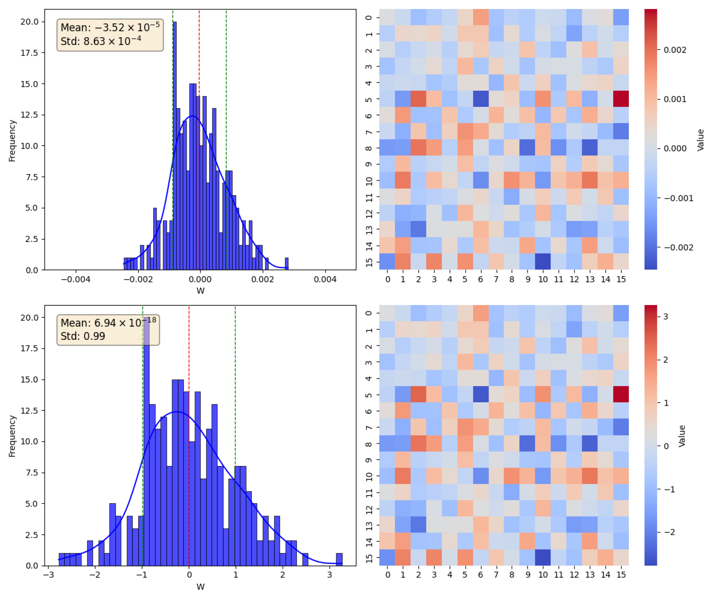
In this section, taking the simple RNN as an example, we analyze the WGN method mathematically. According to the model training process, after normalization, the sparsity of the weight gradient matrix decreases, and the variance approaches 1. The distribution of the weight gradient matrix before and after normalization is shown in Figure 3.

The formula for weight update is shown in Equation (6):

$$w^{iter}=w^{iter-1}-\Delta w^{iter}=w^0-\sum _{i=1}^{iter}\eta \Delta w^i,iter=0,1,\dots ,n$$

(6)

$$\Delta w^i={\displaystyle \frac{\Delta w^i-E\left(\Delta w^i\right)}{\sqrt{Var\left(\Delta w^i\right)}+\delta }}$$

(7)

where w denotes the weight of the model, $w^{iter}$ represents the weights at the iter-th iteration of training, $w^0$ denotes the model’s initialized weights, $\eta$ stands for the learning rate, and $\Delta w^i$ denotes the normalized gradient. Taking the mean on both sides of Equation (6) and considering $E(\eta \Delta w^i)=0$, we obtain Equation (8). After normalization, the mean of the weights remains in a good initial state.

$$E\left(w^{iter}\right)=E\left(w^0\right)$$

(8)

Solving for the variance of both sides of the Equation (6) yields Equation (9):

$$Var\left(w^{iter}\right)=Var\left(w^0\right)+{\eta }^{2}Var\left(\sum _{i=1}^{iter}\Delta w^{\mathrm{i}}\right)-2cov\left(w^0,\eta \sum _{i=1}^{iter}\Delta w^i\right)$$

(9)

Expanding ${\eta }^{2}Var({\sum }_{i=1}^{iter}\Delta w^i)$ yields Equation (10):

$${\eta }^{2}Var\left(\sum _{i=1}^{iter}\Delta w^i\right)={\eta }^2\left(Var\left(\Delta w^1\right)+Var\left(\sum _{i=2}^{iter}\Delta w^i\right)+2cov\left(\Delta w^1,\sum _{i=2}^{iter}\Delta w^i\right)\right)$$

(10)

Since Var$(\Delta w^i)$ is constant at 1 after normalization, and so on, the simplification leads to Equation (11).

$${\eta }^{2}Var\left(\sum _{i=1}^{iter}Var\left(\Delta w^i\right)\right)={\eta }^2\left(iter+2\sum _{i=1}^i\sum _{j=i+1}^{iter}cov\left(\Delta w^i,\Delta w^j\right)\right)$$

(11)

Expanding $cov(w^0,\eta {\sum }_{i=1}^{iter}\Delta w^i$) yields Equation (12).

$$cov\left(w^0,\eta \sum _{i=1}^{iter}\Delta w^i\right)=E\left(\left(w^0-E\left(w^0\right)\right)·\left(\left(\sum _{i=1}^{iter}\eta \Delta w^i\right)-E\left(\sum _{i=1}^{iter}\eta \Delta w^i\right)\right)\right)$$

(12)

Since the values of $E({\sum }_{i=1}^{iter}\eta \Delta w^i)$ and $E(\eta \Delta w^i)$ are 0, the further expansion of $E(w^0·\Delta w^i)$ leads to Equation (13).

$$cov\left(w^0,\sum _{i=1}^{iter}\Delta w^i\right)=\eta \sum _{i=1}^{iter}cov\left(w^0·\Delta w^i\right)$$

(13)

Thus, Equation (9) can be summarized as Equation (14).

$$Var\left(w^{iter}\right)=Var\left(w^0\right)+{\eta }^2·iter+2{\eta }^2·\sum _{i=1}^{iter}\sum _{j=i+1}^{iter}cov\left(\Delta w^i,\Delta w^j\right)-2\eta \sum _{i=1}^{iter}cov\left(w^0·\Delta w^j\right)$$

(14)

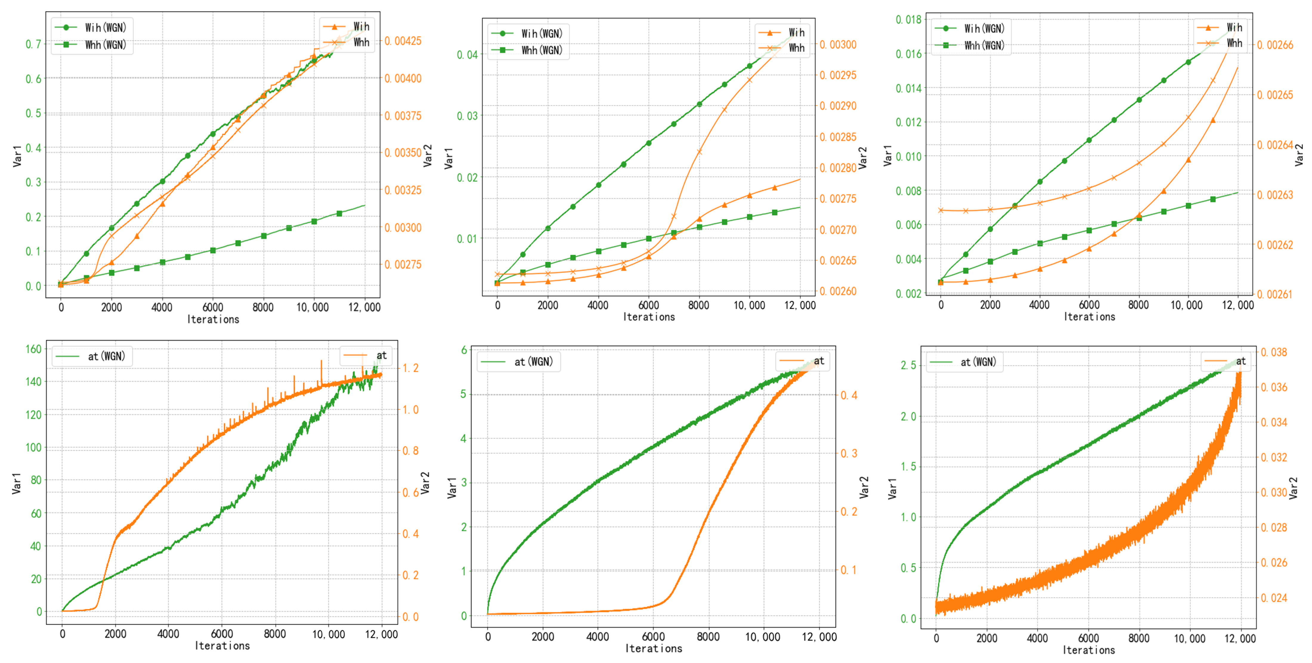
By summing up the last two terms of Equation (14), the sum is found to be close to 0 when choosing a suitable value of $\eta$. There are two cases: one is that $\eta$ is 0, which is obviously impossible, and the other is that $\eta$ satisfies the case as in Equation (15), and there still exists a residual term about iter, and $Var\left(w^{iter}\right)$ can be made roughly linear with iteration, as shown specifically in Figure 4.

$$\left\{\begin{array}{c}\eta ={\displaystyle \frac{2\eta {\sum }_{i=1}^{iter}cov\left(w^0·\Delta w^i\right)}{{\sum }_{i=1}^{iter}{\sum }_{j=i+1}^{iter}cov\left(\Delta w^i,\Delta w^j\right)}}\hfill \\ Var\left(w^{iter}\right)=Var\left(w^0\right)+{\eta }^{2}iter\hfill \end{array}\right.$$

(15)

Equation (16) was used to express the cyclic layer structure of the Simple RNN model.

$$a^t=\sum _{i=1}^{n_I}{w}_{ih}{x}^t+\sum _h^{n_H}{w}_{hh}{h}^{t-1},\forall t,h^t=\theta \left(a^t\right)$$

(16)

where $a^t$ denotes the input of a neuron, $h^{t-1}$ denotes the output of the previous neuron, and $w_{ih}$ and $w_{hh}$ are the parameter weights. Solving for the variance on both sides of the Equation (16) yields Equation (17).

$$Var\left(a^t\right)=Var\left(\sum _{i=1}^{n_I}{w}_{ih}{x}^t+\sum _h^{n_H}{w}_{hh}{h}^{t-1}\right)$$

(17)

Expanding on Equation (17) is more complicated, and we experimentally verified that the neuron outputs of the model under our gradient normalization approach show a more stable upward trend compared to the unnormalized approach, a few cases of which are shown in Figure 4.

During the theoretical derivation, we calculate the covariance of the model weights and their weight gradients, which can be obtained with a small order of magnitude. By comparing the normalized and unnormalized weight variance, it can be found that the parameter variance under the normalized approach changes steadily, which will make the neuron’s output also change steadily, and thus the neuron’s activation probability will not change drastically. In this case, the model can learn the relevant information faster and more steadily. Since the neuron output can stably discard some useless information when passing through the activation function, this leads to a model that is less prone to the gradient explosion and gradient vanishing problems.

4. Dataset

We utilized four datasets, namely the MINIST dataset [11], the PTB dataset [12], the ETTm1 dataset [13], and the UCR dataset [14]. The MINIST dataset comprises 60,000 samples, with 50,000 in the training set and 10,000 in the test set. It is a classic handwritten digital image dataset commonly employed in image classification tasks in machine learning.

The PTB dataset, short for the Penn Treebank dataset, is a classic language model dataset collected and curated by the linguistics department at the University of Pennsylvania as part of the Penn Treebank project. Widely used in language modeling, natural language processing, and other related fields of research, the PTB dataset consists of three text files serving as training, validation, and test sets, containing 929 k, 73 k, and 82 k words, respectively.

The ETT (Electricity Transformer Temperature) dataset collects transformer data from two independent counties in China over two years. We selected the ETTm1 dataset at a 15-min granularity, totaling 69,680 data points, each comprising the target variable “oil temperature” and six power load features. Through sliding windows (which transform time series data into supervised learning datasets), we partitioned it into 48,627 training, 10,303 validation, and 10,303 test instances, training for a total of 20 epochs.

The UCR (Univariate Time Series Classification Archive) serves as an open resource for storing and sharing time series classification datasets. Encompassing various domains and applications such as medicine, finance, and engineering, each dataset contains a set of labeled univariate time series samples, which are categorized based on their time series shapes and features. We selected three datasets from the UCR dataset, coffee, computer, and ECG 500, for training evaluation.

5. Experiment

In the subsequent experiments, we contrasted single-layer and two-layer RNN and LSTM models, with and without weight gradient normalization (WGN), using four different datasets. To emphasize the contribution of WGN, and assuming the program operates normally, we aimed to maintain the original recurrent network models in their simplest configurations possible. Through comparative experiments, specifically contrasting with mini-batch stochastic gradient descent, our objective was to elucidate the performance advantages of the WGN method over traditional approaches. These datasets span multiple domains, enabling a comprehensive evaluation of model performance variations across different data contexts.

5.1. Ablation Experiment

Ablation experiments were conducted using the WGN method on the MINIST dataset, with the parameters $\eta$ set to 0.001 and $\delta$ set to 1 × 10⁻⁵. As illustrated in

Table 1. Comparison of accuracy in WGN ablation experiments.

Method	RNN (1 Layer)	LSTM (1 Layers)
WGN($W_{ih}$)	98.05	98.44
WGN($W_{hh}$)	97.66	98.59
WGN($W_{fc}$)	97.01	98.16
WGN($W_{ih}$) + WGN($W_{hh}$)	98.07	98.56
WGN($W_{hh}$) + WGN($W_{fc}$)	97.84	98.60
WGN($W_{ih}$) + WGN($W_{fc}$)	98.01	98.12
WGN($W_{ih}$) + WGN($W_{hh}$)+WGN($W_{fc}$)	98.04	98.80

, the RNN model is optimally implemented by employing the WGN method on both the $W_{ih}$ and $W_{hh}$. Conversely, the LSTM model is most effectively normalized by applying the WGN method to all weights. Experiments have shown that in some cases, combining gradient normalization for specific weights is more effective than using the WGN method for a particular weight alone. The combination of WGN($W_{hh}$) and WGN($W_{fc}$), as well as the combination of WGN($W_{ih}$) and WGN($W_{hh}$), has been observed to result in a notable enhancement in model performance when compared to their individual normalizations. However, the combination of WGN($W_{ih}$) and WGN($W_{fc}$), when compared to their individual normalizations, has been observed to result in a decline in model performance. It can thus be proposed that a single WGN strategy may not be applicable to all weighty optimization requirements and should be adapted to the specific model structure and task requirements.

5.2. Hyperparametric Sensitivity Analysis

To optimize the model and determine the effective hyperparameter settings for the WGN method in neural networks, a sensitivity analysis of WGN for single-layer neural networks on the MINIST dataset was performed. As illustrated in Table 2, the WGN method yields notable outcomes for RNN neural networks when the value of the parameter $\eta$ is within the range of 0.0001 to 0.001. In the case of LSTM neural networks, the effective range is observed to extend from 0.0001 to 0.005. Furthermore, within the aforementioned effective ranges, an increase in the parameter $\eta$ typically results in enhanced accuracy. In particular, the RNN model attains the highest level of accuracy when the value of $\eta$ is 0.001 and $\delta$ is 1 × 10⁻⁵, whereas the LSTM model demonstrates optimal performance when $\eta$ is 0.005 and $\delta$ is 1 × 10⁻⁴.

The results of our experiments demonstrate that the parameter $\eta$ exerts a more pronounced influence on the WGN method than the parameter $\delta$. Consequently, the selection of suitable hyperparameter values can markedly enhance the optimization of the WGN method, whereas the inappropriate choice of hyperparameters may result in a decline in performance.

Table 2. Comparison of the accuracy of WGN with different combinations of hyperparameters.

	$\mathit{\delta }$	1 × 10−7		1 × 10−6		1 × 10−5		1 × 10−4
$\mathit{\eta }$		RNN	LSTM	RNN	LSTM	RNN	LSTM	RNN	LSTM
0.0001		95.09	96.75	95.35	97.29	94.81	97.18	95.45	96.86
0.0005		97.83	98.28	97.8	98.36	97.74	98.48	97.93	97.98
0.001		97.96	98.60	98.02	98.60	98.04	98.64	97.94	98.63
0.005		58.44	98.88	66.85	98.76	64.75	98.81	48.38	98.91
0.01		11.35	78.29	28.91	97.03	31.06	97.64	10.28	98.90
0.05		9.74	31.95	10.32	28.87	9.82	49.42	10.1	51.06

Table 2. Comparison of the accuracy of WGN with different combinations of hyperparameters.

	$\mathit{\delta }$	1 × 10−7		1 × 10−6		1 × 10−5		1 × 10−4
$\mathit{\eta }$		RNN	LSTM	RNN	LSTM	RNN	LSTM	RNN	LSTM
0.0001		95.09	96.75	95.35	97.29	94.81	97.18	95.45	96.86
0.0005		97.83	98.28	97.8	98.36	97.74	98.48	97.93	97.98
0.001		97.96	98.60	98.02	98.60	98.04	98.64	97.94	98.63
0.005		58.44	98.88	66.85	98.76	64.75	98.81	48.38	98.91
0.01		11.35	78.29	28.91	97.03	31.06	97.64	10.28	98.90
0.05		9.74	31.95	10.32	28.87	9.82	49.42	10.1	51.06

5.3. MINIST Classification

In this paper, we evaluated our models using the MINIST image classification task. For the RNN model, we employed one or more recurrent units with the hyperbolic tangent (tanh) function as the activation function. In the output layer, we extracted the hidden state of the last time step in the sequence and mapped it to the output category dimension through a linear transformation. The LSTM model was similar to the RNN model, and we used the cross-entropy loss function to compute the loss between the model output and the original labels.

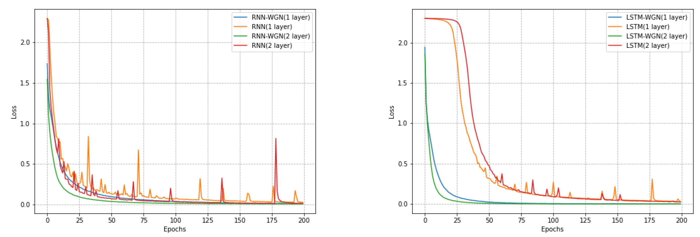
During training, we compared stochastic gradient descent with our own WGN gradient update method, as shown in Figure 5, and the final accuracy comparison is shown in Table 3. Our model featured a recurrent network with 28 time steps, capable of handling information with long-term temporal dependencies. The dimension of the input feature was similarly set to 28. Every 28 × 28 picture was viewed as a sequence in which the order of scanlines was followed to process each row, which represented a row of pixel values in the image. Using a batch size of 1000, a learning rate of 0.05 in the classic gradient descent approach, and 200 training epochs, we selected 128 recurrent hidden units. In the WGN algorithm, we used a scaling factor of 0.001, a bias correction factor of 1 × 10⁻⁵, and the other parameters remained consistent.

5.4. Language Model

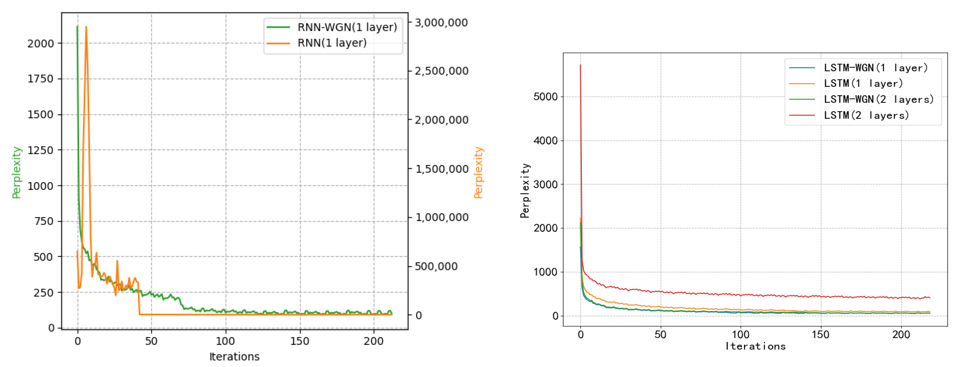
We assessed the models using the PTB dataset at the word level. Our baseline models are LSTM or RNN models with 200 hidden units in each layer. Tanh served as the activation function, and all weight matrices were initialized using a uniform distribution. We used a variable learning rate technique for the unnormalized method: the learning rate (lr) was divided by 4.0, starting at 20 if the current validation loss did not exceed the best validation loss. There are 55 epochs of training in total. The large vocabulary of the PTB dataset may cause serious gradient problems in the RNN network, which could result in program failure. As a result, gradient clipping with a 0.25 clipping coefficient was applied prior to gradient updates. The normalization approach employed a fixed learning rate of 0.0001, while all other parameters stayed the same. As seen in Figure 6, we found that utilizing WGN improved the model’s convergence time even if gradient explosion happened less frequently in LSTM. The final accuracy comparison is shown in Table 4.

5.5. Time Series Prediction Task

In the time series forecasting task, we use the sliding window technique to divide the ETTm1 dataset with an observation window with a length of 126 to obtain a dataset of the new size. We use the mean squared error as a loss function to measure the difference between the predictions and the true values. The task is the multivariate prediction of multivariate, and the model outputs seven dimensions after inputting seven dimensions.

In the recurrent neural network model with 128 hidden units per layer, ReLU was used as the activation function to introduce non-linear relationships. Two predictions were made, one to predict the data for the next 24 time steps and the other to predict the data for the next 96 time steps.

During the training process, the same random seed of 1029 was set, and we divided the data into batches, each of which had a size of 64. We chose the stochastic gradient descent method for the original model without WGN, with the learning rate set to 0.05 to control the magnitude of the model’s update of the weights in each training step, while the learning rate of the normalization method was 0.0001. When we compare the loss variation in Figure 7 to the original baseline, we can see that the WGN significantly improves the RNN model and provides a decent training curve for the LSTM model. The final accuracy comparison is shown in Table 5 suggests that WGN has a good potential to improve the performance and efficiency of models in time series prediction tasks.

5.6. Time Series Classification Task

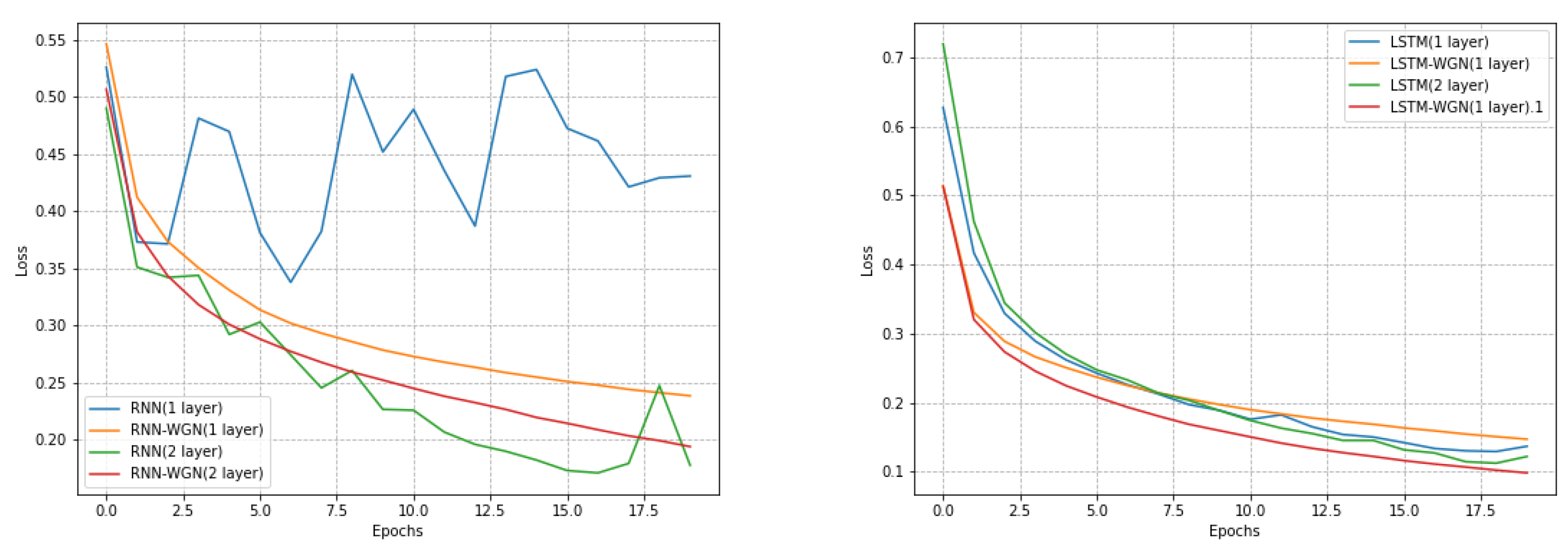
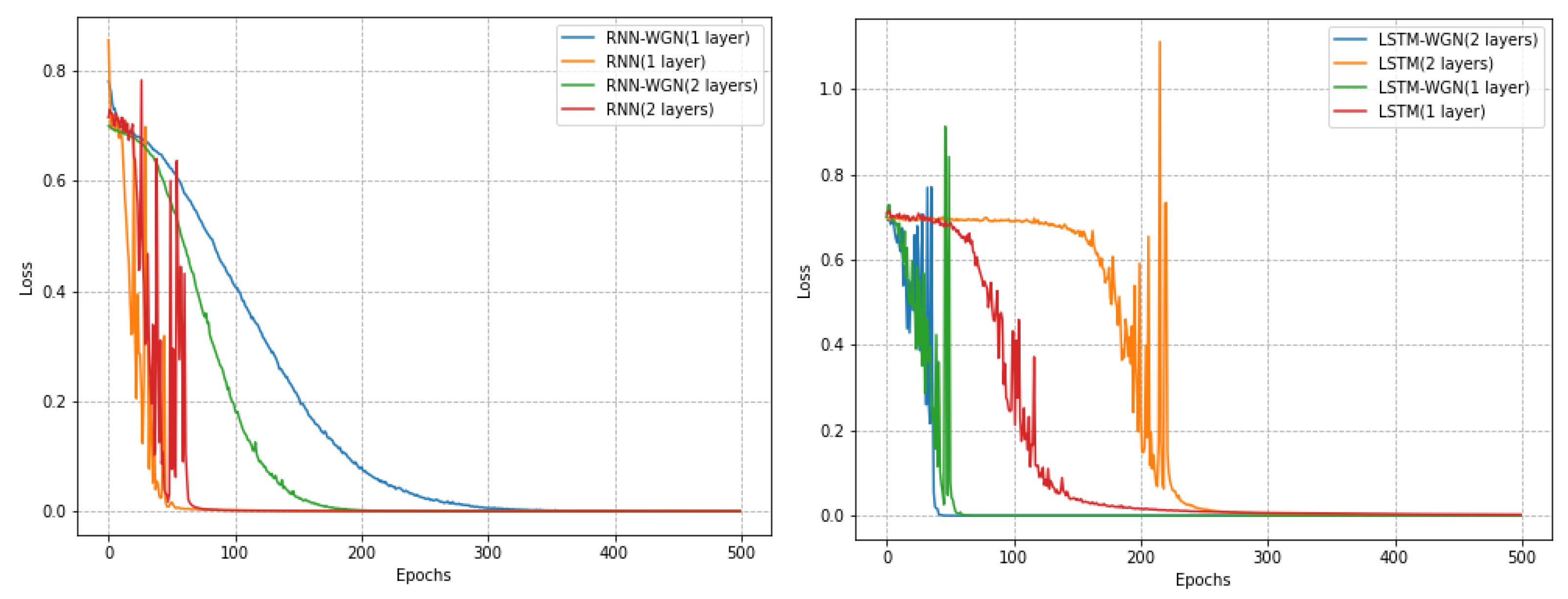
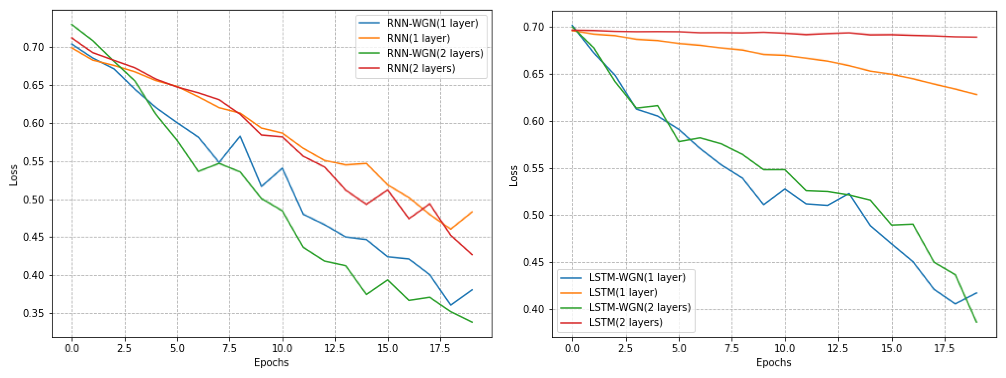
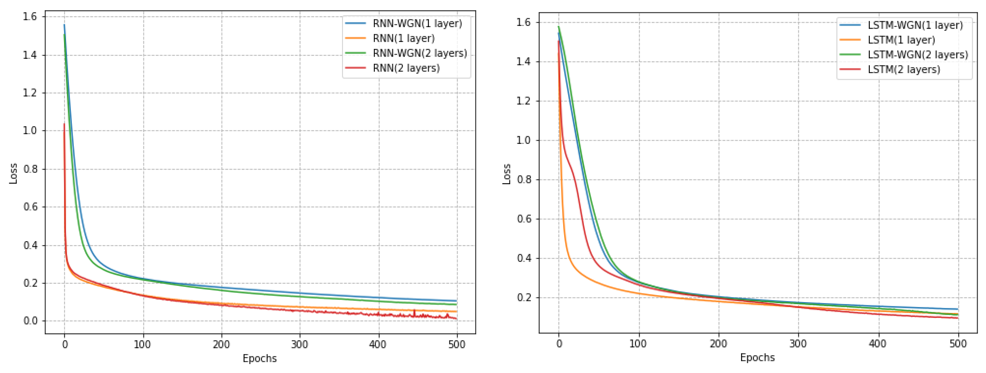
In our time series classification task, we selected three datasets from the UCR dataset. With the same stochastic seed, these three datasets have a smaller sample size, a learning rate of 0.05 for stochastic gradient descent, and a learning rate of 0.0001 for the WGN method. For the Coffee and ECG5000 datasets, we trained a total of 500 epochs, while for the Computers dataset, we trained only 20 epochs. We found that on the Computers dataset, the model achieved better performance with fewer training rounds.

Notably, on the Coffee dataset, the RNN model using the WGN method exhibited a smoother learning process, while the LSTM model demonstrated faster convergence. Although the WGN method did not effectively solve the gradient problem in the Computers dataset, it still accelerated the convergence of the models. In the ECG5000 dataset, the WGN method was not as effective but still improved the best accuracy by about 0.4 percent. As shown in Figure 8, Figure 9 and Figure 10 and Table 6, our experimental results indicate that different datasets may require different optimal training strategies. The WGN method exhibits a smooth learning process and faster convergence in most cases, showing the potential to improve the performance of time series classification.

6. Metric

We designed a metric LOE to measure the gradient problem, where $los{s}_t$ denotes the loss value at moment t, epoch denotes the current training round, and total_epoch denotes the total number of training rounds.

$$\mathrm{LOE}=\left|{\displaystyle \frac{{loss}_t-{loss}_{t-1}}{{loss}_{t-1}+\alpha }}\right|·e^{{\displaystyle \frac{\rho ·\mathrm{epoch}}{\mathrm{total}\_\mathrm{epoch}}}}$$

(18)

As training proceeded, we noticed that the negative impact of the gradient problem on model training gradually increased in the later stages of training. In order to quantify this, we designed a correction mechanism containing an exponential term for correcting the severity of the gradient problem. In the index we designed, the parameter LOE represents the degree of impact of the gradient problem on training, with larger values indicating a more significant impact of gradient explosion. Specifically, we first calculated the proportion of the increase in loss at each time node relative to the previous time node; this proportion requires an absolute value operation because both gradient vanishing and gradient explosion can occur. We then multiplied this proportion by an e-exponential correction term, where the value of the exponent is related to the number of training rounds and model parameters. By introducing such a correction mechanism, we can more accurately visualize the extent to which the model is experiencing gradient problems and can effectively improve the model based on these indicators. The performance comparison of the models using WGN and without WGN method is shown in Table 3, Table 4, Table 5 and Table 6 and the performance comparison of using the WGN method with gradient clipping and the GRU model is shown in

Table A1. Comparison of the WGN method with gradient clipping and the GRU method on the MINIST dataset. Bolded values are for best performance.

Metric	RNN-CLIP		LSTM-CLIP		GRU		LSTM-WGN
	1 Layer	2 Layers	1 Layer	2 Layers	1 Layer	2 Layers	1 Layer	2 Layers
Accuracy	98.09	98.30	98.07	98.42	98.35	98.71	98.80	99.11
LOE	68.05	97.27	46.44	40.50	66.36	49.62	55.15	25.90

and

Table A2. Comparison of the WGN method with gradient clipping and the GRU method on the PTB dataset. Bolded values are for best performance.

Metric	LSTM-CLIP		GRU-CLIP		LSTM-WGN
	1 Layer	2 Layers	1 Layer	2 Layers	1 Layer	2 Layers
PPL	110.76	109.49	119.30	127.72	118.58	110.89
LOE	55.12	55.59	54.88	56.05	55.15	54.78

. Their experimental configurations are all the same as those described in the previous experimental section.

Table 3. Best metric on the training and development sets on MINIST. Bolded values are for best performance.

Metric	RNN		RNN-WGN		LSTM		LSTM-WGN
	1 Layer	2 Layers	1 Layer	2 Layers	1 Layer	2 Layers	1 Layer	2 Layers
Accuracy	98.07	98.21	97.91	98.04	97.94	98.42	98.80	99.11
LOE	57.63	132.49	9.39	16.42	27.62	17.22	55.15	25.90

Table 3. Best metric on the training and development sets on MINIST. Bolded values are for best performance.

Metric	RNN		RNN-WGN		LSTM		LSTM-WGN
	1 Layer	2 Layers	1 Layer	2 Layers	1 Layer	2 Layers	1 Layer	2 Layers
Accuracy	98.07	98.21	97.91	98.04	97.94	98.42	98.80	99.11
LOE	57.63	132.49	9.39	16.42	27.62	17.22	55.15	25.90

Table 4. Best metric on training and development sets on Peen Treebank. Bolded values are for best performance.

Metric	RNN		RNN-WGN		LSTM		LSTM-WGN
	1 Layer	2 Layers	1 Layer	2 Layers	1 Layer	2 Layers	1 Layer	2 Layers
PPL	383.20	972.38	144.97	141.02	125.27	293.15	118.58	110.89
LOE	37.77	104.59	58.05	54.52	53.14	55.62	55.15	54.78

Table 4. Best metric on training and development sets on Peen Treebank. Bolded values are for best performance.

Metric	RNN		RNN-WGN		LSTM		LSTM-WGN
	1 Layer	2 Layers	1 Layer	2 Layers	1 Layer	2 Layers	1 Layer	2 Layers
PPL	383.20	972.38	144.97	141.02	125.27	293.15	118.58	110.89
LOE	37.77	104.59	58.05	54.52	53.14	55.62	55.15	54.78

Table 5. Best metric on training and development sets on ETTm1. Bolded values are for best performance.

Metric		RNN		RNN-WGN		LSTM		LSTM-WGN
		1 Layer	2 Layers	1 Layer	2 Layers	1 Layer	2 Layers	1 Layer	2 Layers
len = 24	MAE	0.806	0.943	0.978	0.886	0.802	0.866	0.778	0.902
	LOE	34.62	81.15	8.28	13.85	23.78	32.58	15.29	24.00
len = 96	MAE	0.635	0.733	0.592	0.678	0.681	0.685	0.704	0.790
	LOE	9.94	17.58	6.38	11.83	20.03	27.33	14.63	21.95

Table 5. Best metric on training and development sets on ETTm1. Bolded values are for best performance.

Metric		RNN		RNN-WGN		LSTM		LSTM-WGN
		1 Layer	2 Layers	1 Layer	2 Layers	1 Layer	2 Layers	1 Layer	2 Layers
len = 24	MAE	0.806	0.943	0.978	0.886	0.802	0.866	0.778	0.902
	LOE	34.62	81.15	8.28	13.85	23.78	32.58	15.29	24.00
len = 96	MAE	0.635	0.733	0.592	0.678	0.681	0.685	0.704	0.790
	LOE	9.94	17.58	6.38	11.83	20.03	27.33	14.63	21.95

Table 6. Best metric on training and development sets on UCR. Bolded values are for best performance.

Metric		RNN		RNN-WGN		LSTM		LSTM-WGN
		1 Layer	2 Layers	1 Layer	2 Layers	1 Layer	2 Layers	1 Layer	2 Layers
ECG5000	Accuracy	0.935	0.932	0.939	0.939	0.935	0.933	0.930	0.925
	LOE	192.791	2446.467	29.486	52.538	56.822	86.378	25.096	63.990
Coffee	Accuracy	0.964	0.964	0.964	0.964	1.000	1.000	1.000	1.000
	LOE	35.237	68.573	67.513	27.677	35.013	64.383	86.321	25.374
Computers	Accuracy	0.600	0.524	0.556	0.572	0.652	0.600	0.624	0.660
	LOE	18.627	27.378	27.817	23.865	3.876	0.543	20.221	26.314

Table 6. Best metric on training and development sets on UCR. Bolded values are for best performance.

Metric		RNN		RNN-WGN		LSTM		LSTM-WGN
		1 Layer	2 Layers	1 Layer	2 Layers	1 Layer	2 Layers	1 Layer	2 Layers
ECG5000	Accuracy	0.935	0.932	0.939	0.939	0.935	0.933	0.930	0.925
	LOE	192.791	2446.467	29.486	52.538	56.822	86.378	25.096	63.990
Coffee	Accuracy	0.964	0.964	0.964	0.964	1.000	1.000	1.000	1.000
	LOE	35.237	68.573	67.513	27.677	35.013	64.383	86.321	25.374
Computers	Accuracy	0.600	0.524	0.556	0.572	0.652	0.600	0.624	0.660
	LOE	18.627	27.378	27.817	23.865	3.876	0.543	20.221	26.314

In the language models, the perplexity of the models utilizing WGN is typically lower than that of the models not employing WGN. Moreover, both the perplexity and the LOE of the models utilizing WGN demonstrated a decline as the number of layers increased. The perplexity reached a minimum in the two-layer LSTM model with WGN, and the LOE was found to be average. In the context of the image dataset classification, the highest accuracy was observed when the WGN method was employed with a network comprising two layers, utilizing either the RNN or the LSTM model. Furthermore, the incorporation of the WGN method into the RNN model resulted in a significant reduction in the LOE. In contrast, the introduction of WGN into the LSTM model led to a notable enhancement in accuracy, although this was accompanied by an increase in LOE. For the prediction task of the ETTm1 dataset, we observed that the performance of recurrent neural networks or LSTM models with different numbers of layers combined with the WGN method varied under different prediction length conditions. Firstly, at a prediction length of 96, the two-layer RNN-WGN model exhibited the lowest mean absolute error, while the single-layer RNN-WGN model demonstrated the lowest LOE. Conversely, at a prediction length of 24, the one-layer LSTM-WGN model exhibits the most favorable outcomes, while the one-layer RNN-WGN model demonstrates the lowest LOE. This indicates that the utilization of the WGN approach is an effective method for optimizing model performance and achieving optimal values in different settings. It can be observed that the model with WGN exhibits markedly elevated accuracy and markedly reduced LOE in the ECG5000 dataset. In the Coffee dataset, the two-layer LSTM-WGN model demonstrates the optimal LOE, although the accuracy is not significantly enhanced. In the Computer dataset, the two-layer LSTM-WGN model attains the highest accuracy.

7. Conclusions

This paper presents an analysis of the causes of the gradient problem from the perspectives of gradient variance and covariance. It also proposes a new gradient updating method and an evaluation metric to quantify the gradient problem based on statistical theory. The efficacy of the WGN method in alleviating the gradient problem in deep neural networks, particularly recurrent neural networks and networks with long time-dependent characteristics, has been demonstrated through experimentation on multiple public datasets. In addition to suppressing the gradient problem, the WGN method has been shown to accelerate model convergence and improve accuracy. Furthermore, it is our contention that the WGN algorithm requires further examination in the following instances:

(1) Our findings indicate that the implementation of the WGN method in a single-layer RNN neural network does not result in a notable enhancement in the accuracy rate. However, the LOE index of the model exhibits a considerable improvement. This is due to the monotonous structure of the single-layer Simple-RNN, which produces a permutation effect on the LOE metrics and accuracy.

(2) In some cases, the use of the gradient normalization method has been observed to occasionally result in a decrease in accuracy or an increase in LOE metrics when applied to smaller datasets. This is primarily attributable to the fact that the batch size is constrained when the dataset is limited in size. This results in an incomplete representation of the overall sample probability within the sample space corresponding to each batch, which in turn gives rise to an increase in the discrepancy between the batches and affects the robustness of the training process. In small-scale datasets where the variability of samples is stronger, the use of gradient normalization may result in an over-adjustment of the gradient, which in turn affects the overall performance of the model. In contrast, in large-scale corpus datasets, the WGN method is more likely to capture the overall characteristics of the gradients and effectively balance the gradient differences between different samples.

(3) The necessity for the additional computation of the mean and variance of the gradient for each batch inherent to the gradient normalization method also results in an increase in time complexity. It is therefore not recommended that the gradient normalization method be employed in scenarios where there is a high requirement for real-time processing and a low requirement for accuracy.

In general, the models incorporating WGN appear to yield the most favorable outcomes across a range of tasks. This suggests that the WGN approach has broad applicability and can provide effective support for the training of diverse types of models. In future research, we will continue to investigate the efficacy of WGN and apply it to a broader range of models, including GRU and Transformer.