Article

The Geographic Automata Tool: A New General-Purpose Geosimulation Extension for ArcGIS Pro

by
Alysha van Duynhoven
* and
Suzana Dragićević
Spatial Analysis and Modeling Laboratory, Department of Geography, Simon Fraser University, 8888 University Drive, Burnaby, BC V5A1S6, Canada
*
Author to whom correspondence should be addressed.
Appl. Sci. 2024, 14(15), 6530; https://doi.org/10.3390/app14156530
Submission received: 12 June 2024 / Revised: 11 July 2024 / Accepted: 11 July 2024 / Published: 26 July 2024
(This article belongs to the Special Issue Geospatial Technologies in Spatial and Environmental Planning)

Abstract

:
The theoretical paradigm of geographic automata systems (GAS) underpins a wide range of studies to represent dynamic complex geospatial phenomena. Specifically, cellular automata (CA) were used extensively over the past 40 years for geospatial applications, though primarily for modeling urban growth. Currently, the hyper-specialized and fragmented geospatial technology ecosystem supporting CA model implementation often necessitates programmed solutions or use of disconnected programs with graphical user interfaces (GUIs) separate from common geographic information systems (GIS) software. Therefore, the main goal of this study is to present a general-purpose, GIS-based CA modeling framework and extension for Esri’s ArcGIS Pro software environment. The methodological approach centered around (1) developing generic functions for building binary or multi-class CA models to capture various spatiotemporal systems and (2) enabling end-to-end CA modeling projects that can incorporate built-in functionality available in ArcGIS Pro versions 3.1 and newer. Two case studies demonstrate the add-in capabilities to support geosimulation model-building activities and exploration of new hybrid models. This research contributes to advancing flexible, transparent spatiotemporal modeling tools within existing GIS software. The proposed approach addresses the lack of streamlined geospatial technologies capable of simulating numerous dynamic geospatial phenomena, exploring human and environmental processes, and examining possible futures with CA in research, decision making, or educational settings.

1. Introduction

Geographic automata systems (GAS) are a longstanding theoretical framework used to represent and model complex dynamic geospatial phenomena [1]. Since its introduction, this spatiotemporal modeling paradigm continues to be an important research theme within the domain of geographic information science (GIScience) [2]. By portraying local-level processes and interactions, GAS models support investigation of change mechanisms that produce larger-scale patterns [3]. Additionally, their capacity to depict complex systems behaviors like non-linearity, emergence, and feedback loops offers benefits over top-down statistical modeling strategies [4]. Within the GAS paradigm, cellular automata (CA) and agent-based modeling (ABM) approaches are used for simulating local and individual dynamics, respectively, from the bottom up [1]. Of the two strategies, CA modeling is utilized extensively due to lower technical barriers, less stringent data requirements, flexibility of expression, and theoretical simplicity [5]. Such characteristics also make the paradigm more accessible to multi-disciplinary researchers beyond the field of geography.
Geographic CA extends traditional elements of CA conveyed in earlier studies [6,7] to include grids of regularly or irregularly spatially tessellated cells, discrete cell states, neighborhood functions, transition rules, and discrete increments of time [8,9,10,11]. Simple transition rules capturing local interactions are used to simulate the behaviors of geospatial systems [12], examine processes [10], explore “what-if” scenarios [13], assist in spatial and environmental planning endeavors [14], and support spatial decision-making practices [15]. The nature of CA also allows seamless integration of geospatial data acquired from remote sensing (RS) imagery or raster GIS datasets [16,17]. Although adjustments to essential model elements can facilitate representation of innumerable real-world systems [6], studies leveraging the geographic CA paradigm mainly focus on land change simulation [2,18], especially urban growth [3,19,20]. Even so, CA were successfully used to model a range of geospatial phenomenon like human epidemics [21], deforestation [22], forest fires [23], insect infestation [24,25], snow cover extent [26], seismicity [27], sand dune dynamics [28], and avalanches [29]. However, the commonality among the listed pursuits is their programmed implementations.
Whether code for each study is openly available or not, programming is a recurring barrier in developing CA models that are explicitly spatial and compatible with geospatial data. Several efforts to create standalone and integrated geographic CA modeling tools equipped with graphical user interfaces (GUIs) sought to expediate model implementation and reduce technical obstacles. Reflecting the dominant usage of geographic CA models in urban land change applications, numerous GUI-based CA software applications specialized for this phenomenon have included SLEUTH [30], DUEM [31], UrbanSim [32], Metronamica [33], and FLUS [34]. However, standalone CA tools typically encapsulate fragments of model-building activities, requiring tasks like data preparation, geospatial analyses, and cartography to be conducted using other solutions [35]. For example, previous studies employed ad hoc model-building procedures spanning multiple software and programmatic solutions [36,37,38].
To alleviate tool-switching bottlenecks, studies proposed new extensions or “add-ins” created for familiar GIS software environments. An early example of this is SimLand, which was created to extend Esri’s ArcInfo software [39]. Since then, several works offered specialized extensions for Esri’s ArcGIS Desktop software such as iCity [35], GeoSOS [40], BNID-CA [41], and WDUNE [28]. Other CA add-ins extended functionality of Idrisi Kilimanjaro [42] and QGIS [43] for modeling forest fires and land change, respectively. Nevertheless, both standalone and add-in tools routinely exhibit limited capacity to represent other geospatial systems and are often not updated for use in newer GIS software environments. Additionally, fundamental components of geographic CA models like neighborhood functions or transition rules are repeatedly disconnected from theoretical terminology, lack flexibility, are entirely hard-coded, or are replaced with black-box mechanisms that impede transparency necessary for supporting real-world decision making. Consequently, the rigidity and black-box nature of many specialized GUI-based CA modeling tools alienate multi-disciplinary researchers who may have benefited from even basic model-building functionality.
To address the hyper-specialized, fragmented, and programmer-centric nature of modern geospatial technologies and workflows supporting CA, the main goal of this study is to develop a general-purpose, user-friendly geosimulation modeling tool accessible in a contemporary GIS software environment. The proposed framework and add-in functions should support end-to-end CA model-building activities, which include data pre-processing, model parameterization, model execution, model evaluation, and visualization of simulation outcomes. To meet the primary objective, this research describes the design and development of the Geographic Automata add-in. The add-in is compatible with ArcGIS Pro 3.1 and newer versions. The proposed framework and features aim to (1) provide generic functions for creating binary or multi-class representations of various geospatial systems and (2) facilitate end-to-end model-building workflows that can be entwined with ArcGIS Pro functionality. The utility and capabilities of the Geographic Automata add-in are demonstrated via two case studies involving hypothetical and real-world geospatial datasets. The first case study focuses on multi-class insect infestation modeling encoded with previously reported behaviors, while the second case study introduces the inaugural use of automated machine learning (AutoML) with CA to inform urban growth allocations.

2. Brief Overview of Geographic CA Modeling and Tools

The essential function of geographic CA modeling tools is to support flexible configuration of five key elements (grids of cells, cell states, neighborhood functions, transition rules, and discrete time). In general, a CA can be expressed as follows [17]:
S T + 1 = { S T ,   N T ,   F T , T }
where the new cell state ( S T + 1 ) at time T + 1 depends on cell state S T at the initial time T , the cell’s neighborhood ( N T ), the transition rules ( F T ), and the discrete time represented by the temporal interval corresponding with one iteration of the model ( T ). A CA model is run in a stepwise manner, where the grid of cells, cell states, neighborhood functions, and transition rules that generate or limit changes are stored in an intermediate data layer [44]. At the end of an iteration, intermediate cell states are added to the output data layer together [45,46]. A geographic CA is spatially explicit because it is directly linked to georeferencing principles that determine the location of the cells and their connection to Earth’s physical surface. As such, it innately links geospatial data as raster GIS data layers that govern the cell states. Each iteration output can then be represented as a map generated from the spatiotemporal model simulation.

2.1. Typical CA Transition Rule Mechanisms

Transition rules combine key geographic CA elements—the structural grid of cells, possible cell states, and neighborhood compositions—to mechanize geospatial processes that generate changes over time [8]. However, transition rules seldom rely exclusively on a cell’s current state and those of its neighbors for propagating changes [47]. Instead, change events are typically produced or constrained based on current cell states, neighborhood characteristics, outcomes of other spatial or aspatial analyses, or global-level settings [11,48,49]. One now-ubiquitous strategy in geographic CA modeling is to integrate products of other spatial or aspatial analyses in transition mechanisms. For instance, studies have guided transition rule behaviors with suitability or susceptibility maps outputted by techniques like multi-criteria evaluation (MCE) [48,49], or probability maps produced by machine learning (ML) classifiers [20,38,50]. Other studies involved estimated values produced with geographically weighted regression (GWR) to influence allocation of new changes [51]. Likewise, simply adding stochasticity to CA rule mechanisms was used to produce non-deterministic simulation outcomes [10,44,52], to portray the inherent uncertainty of real-world processes and anthropogenic activities [53], and to accommodate lack of complete information about system behaviors [9]. Alongside suitability maps and stochastic terms, global limits on the number of changes were also set to constrain a model’s behavior [50,54,55] and used to implement “what-if” scenarios [37]. Other studies set spatial constraints to prevent changes within certain locations [55] and to examine the effects of policies [56]. Therefore, a general-purpose modeling tool should support implementations of CA transition rule extensions without requiring users to abandon transparency unless they choose to.

2.2. Previous General-Purpose CA Modeling Tools

Currently, there are few general-purpose, explainable CA modeling tools usable for representing various geospatial phenomena. One example is SpaSim [57], a spatial modeling tool developed to overcome requirements of programming skills and the specialization of CA tooling already observed thirty years ago. Since then, the Dinamica Geoprocessing Objects (EGO) software [45] was presented as an openly available geosimulation modeling solution with phenomena-agnostic functionality. However, the introductory documentation, expansive and jargon-filled functor list, and interface design pose difficulties for users unacquainted with GIS analysis terminology or other GIS software. CA model-building workflows are also possible within the TerrSet 2020 GIS software [58] using the Macro Modeler, CELLATOM module, and the experimental (and problematic) CA-Markov module [59]. For example, the Macro Modeler supported CA model implementation of landslides [49] and insect infestation scenarios [60]. Still, the TerrSet GIS software is challenging for users who are unfamiliar with performing raster GIS operations, preparing data for use in different GIS software environments, resolving ambiguous and often undocumented errors, and navigating the legacy UI design. Furthermore, initial hands-on model-building experiences are often negatively impacted by the disconnection of rote implementation and theory of geographic CA. When scientific procedures are predominately composed of memorized, unintuitive procedures, beginners avoid experimenting beyond the guiderails they were taught [61]. Hence, geographic CA modeling tools directly linked to key terminology and integrated within existing GIS software environments would better support users of all skill levels.

2.3. Essential Elements of GUI-Based Geographic CA Modeling Tools

To build and implement a geographic CA model in a GIS software environment, add-in tools must have facilities for defining neighborhood functions, a structure for specifying transition rules, and a means of applying transition rules in a synchronous [62] or asynchronous manner [63]. Previous studies also outlined CA modeling tool requirements such as input and output specification options [10], interactivity [64], and user-friendly GUIs [42]. Though earlier GUI-based standalone applications had functions for displaying previously simulated timesteps [57] or recreated basic GIS functionalities to support CA modeling workflows [45], development endeavors that extend existing GIS software benefit from the built-in data visualization, input, storage, and processing functions. As such, programming efforts can be solely focused on creating CA modeling tools. In addition to implementing CA model elements, GUI-based tools often support model evaluation adhering to the broader tradition of comparing simulated outcomes and real-world data [65]. For example, prior CA modeling tools supplied small sets of map comparison metrics including overall accuracy, various Kappa metrics, and the Figure of Merit (FOM) [34,43]. Overall, a general-purpose add-in should support users in configuring key model elements, executing model routines, and conducting basic model evaluation to facilitate end-to-end model-building activities within an established GIS software environment.

3. Methodology

The Geographic Automata add-in was developed using the C# programming language [66] and the ArcGIS Pro Software Development Kit (SDK) for .NET [67]. In the balance between generality, realism, and precision [68], the add-in implementation aimed to maximize generalization of essential modeling functionality outlined in Section 2. The main operations are implemented in three tool groups called Model Parameterization, Model Execution, and Model Evaluation (Figure 1a). The functions support end-to-end binary (Figure 1b) and multi-class CA modeling workflows (Figure 1c).

3.1. Model Parameterization

The Model Parameterization tool group hosts functions for defining neighborhoods and transition rules. These simple elements underpin the built-in parameterization options in the Basic CA tool and serve as “building blocks” for customizing Advanced CA model behavior.

3.1.1. Specifying Neighborhood Functions

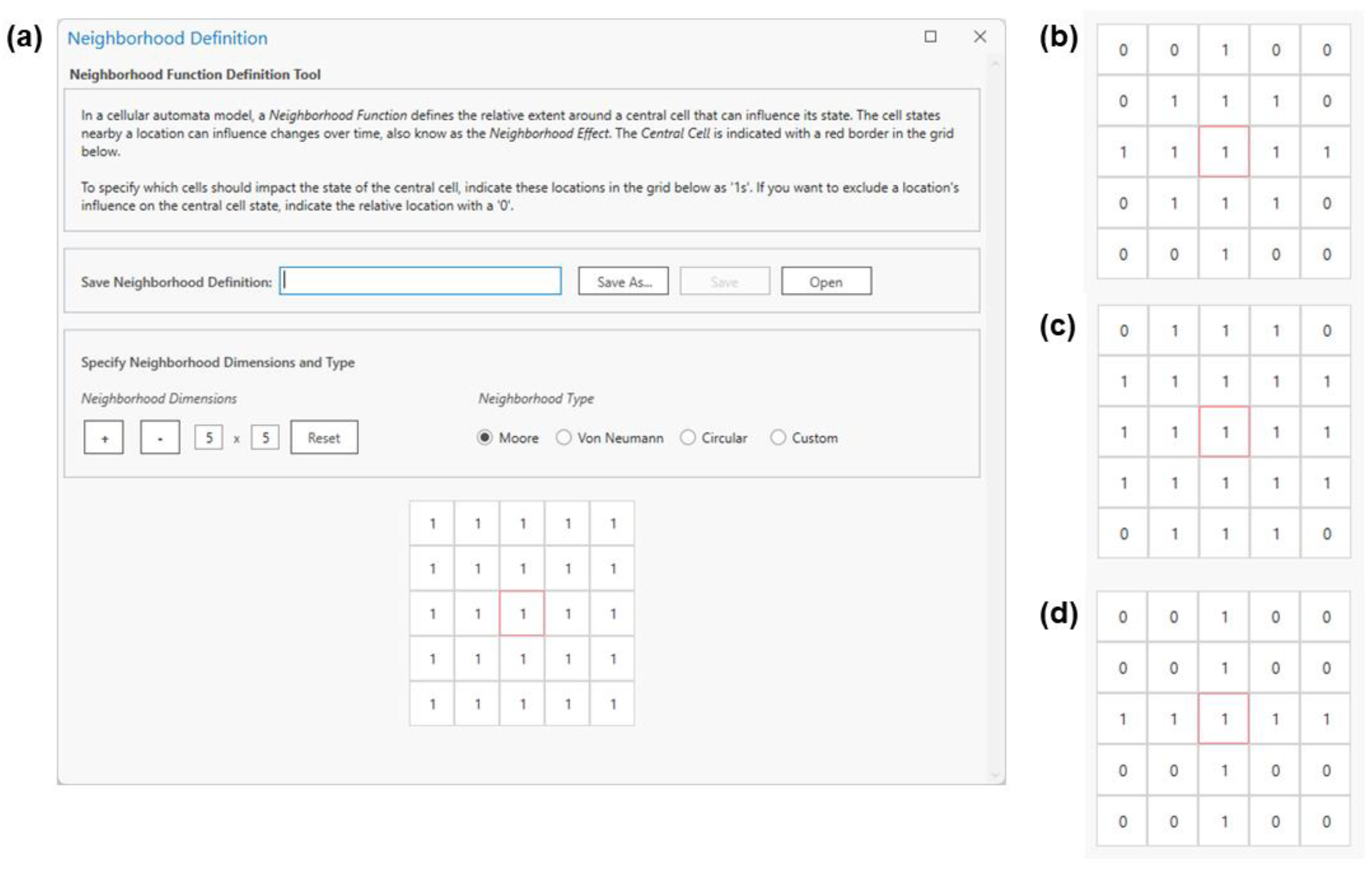
The Neighborhood Definition tool supports GUI-based neighborhood function specification (Figure 2a). The most common neighborhood configurations—Moore, Von Neumann, and circular [53]—are available as preset options. Additionally, a Custom neighborhood option supports manual specification of alternatives like linear [69], ring-shaped [70], and simple directional configurations [25] (Figure 2d). Neighborhood functions are saved as Neighborhood Definition files (*.nb) for use in transition rule definitions described in the next section.

3.1.2. Specifying Transition Rules

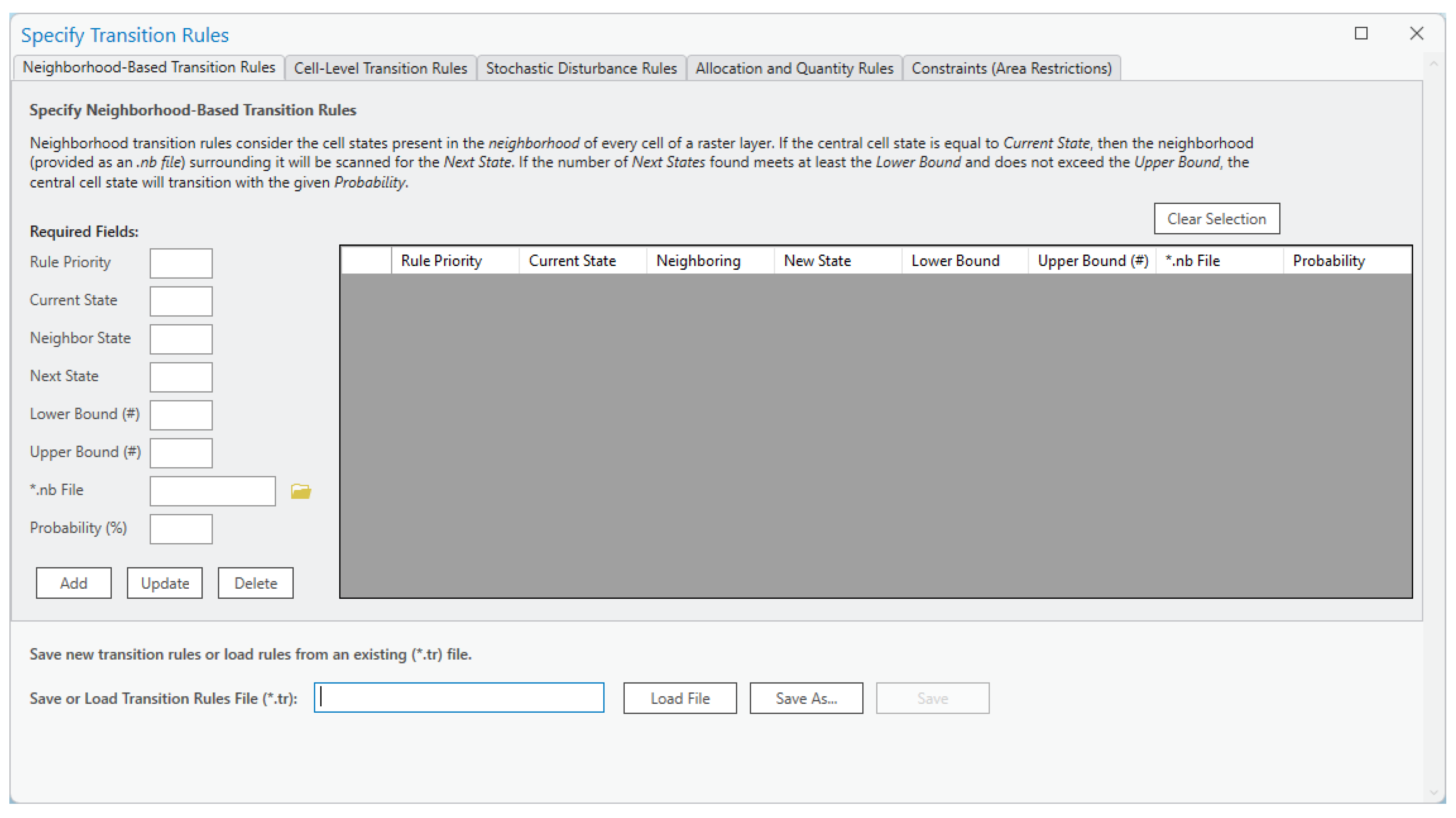
The Specify Transition Rules tool was developed to facilitate specification of explainable rule tables. Through a rule table structure [71], users can trace rule mechanisms that generate larger-scale patterns. The tool interface supports typical “create, read, update, and delete” (CRUD) operations applied to Transition Rule files (*.tr) produced by the tool. There are no limits to the number of rules users can specify in Transition Rule files. Once a Transition Rule file is specified, it can be provided to the Advanced CA tool described in Section 3.2.
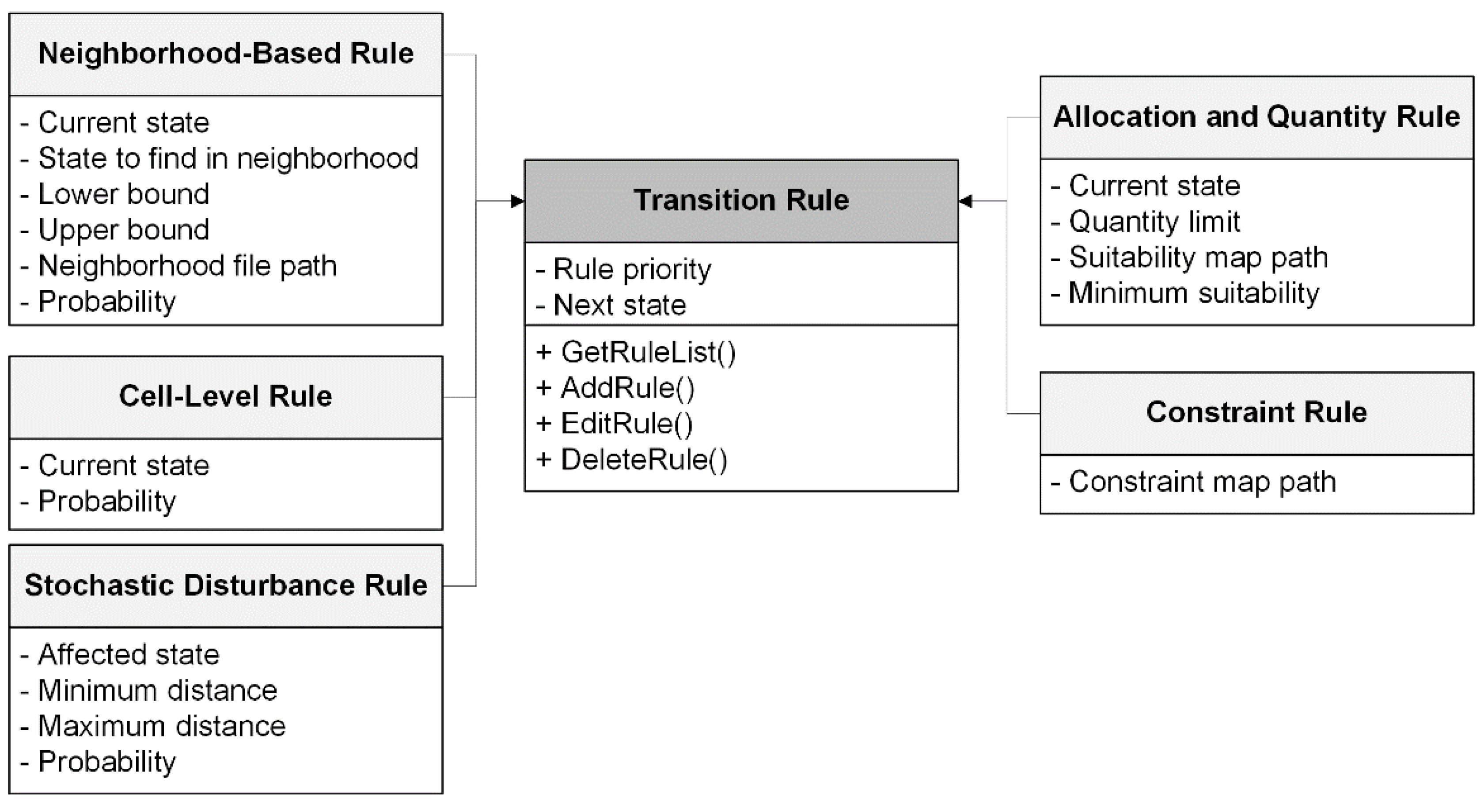
The initial version of the Geographic Automata add-in supports five basic transition rule types that either generate or limit potential transitions based on previous works (Section 2.1). Generative rules include Neighborhood-Based, Cell-Level, and Stochastic Disturbance rules, while Allocation and Quantity and Constraint rules limit propagation of changes (Figure 3). Figure 4 presents the UML diagram of Transition Rule objects, which require a current state, the next state, and rule conditions. The generative rule types also offer a Probability parameter that can be set to 100% to ensure deterministic behaviors. All rule types operate by modifying an intermediate raster grid before producing the outcome for the model iteration or timestep.

Neighborhood-Based Rules

A Neighborhood-Based rule is used to propagate changes based on neighborhood conditions. Rules of this type require a current state ( S T ), the possible next state ( S T + 1 ), the cell state to search for within each cell’s neighborhood ( S T N ), a neighborhood function ( N T ) provided as an *.nb file, neighborhood composition conditions ( min S T N m a x ), and the likelihood of the transition to occur ( Ρ ). Numerous Neighborhood-Based rules can be specified to represent behaviors for each cell state or class [72], to capture varying influences at different neighborhood extents [31], or to set separate transition probabilities for specific neighborhood conditions [11]. Additionally, the next state ( S T + 1 ) is not required to be the same as the cell state being searched for in the cell’s neighborhood ( S T N ). This supports portrayal of behaviours like “road-influenced growth” [30,73], varying urban expansion patterns depending on nearby land use types [74], or presence of snow cover nearby [75].

Cell-Level Rules

A Cell-Level rule is used to instigate changes based exclusively on a cell’s current state. Rules of this type require a current state ( S T ), the possible next state ( S T + 1 ), and the likelihood of the transition to occur ( Ρ ). A Cell-Level rule can implement cell-level changes such as eventual plant death or exhaustion of resources [76], wildfire progression from newly burning, growing, to extinguished [77,78], or spontaneous urban growth without proximity requirements [73].

Stochastic Disturbance Rules

While modeling some phenomena may benefit from global random disturbance mechanisms, propagation of change is more often driven by nearby conditions [64]. A Stochastic Disturbance rule is used to generate changes at locations featuring some “affected state” ( S T a ) within some cell distance ( d m i n , d m a x ) from an “emitter state” ( S T e ) with a given probability ( Ρ ). The possible next state of an affected cell is equivalent to S T + 1 = S T e . Each “edge cell” of the emitter state is permitted to propagate one stochastic disturbance if the probability mechanism is satisfied and if the potential change does not violate the minimum distance requirement of other emitter cells. A Stochastic Disturbance rule can be used to implement behaviors like forest fire spotting [23] or invasive plant species propagation [76].

Constraint Rules

Constraint rules prevent transitions related to a specific cell state from occurring within restricted areas. Rules of this type require a potential next state ( S T + 1 ) and a binary raster map indicating where cells are barred from becoming S T + 1 [48]. With Constraint rules, users can easily add, swap, or delete areal restrictions to explore different scenarios or spatial policies [56].

Allocation and Quantity Rules

Allocation and Quantity rules guide the location and amount of specific from-to transitions through suitability maps and quantity limits. With this rule type, prospective changes can be limited to the most suitable or susceptible locations identified using analyses like MCE [79], or those corresponding to locations with higher probabilities outputted by ML classifiers [55]. Allocation and Quantity rules require users to specify a cell’s current state ( S T ) and the potential next cell state ( S T + 1 ). Unlike other rule types, Allocation and Quantity rules have three modes (Table 1). Optional fields for each mode include a minimum suitability threshold ( m i n m ), a path to a suitability, susceptibility, or probability map ( M ), and an integer ( Q ) indicating the maximum quantity of cells permitted to transition at each discrete timestep or model iteration ( T ).

Rule Priority Scheme

With the Rule Priority field, users can override the default order of generative rule execution at each model iteration (Figure 5). The purpose is to support prioritization of change mechanisms and to maintain explainable model behavior, especially in multi-class model implementations. For example, a less common but important transition occurring in specific situations could be eliminated by competing rules that propagate more widespread or probable change behaviors.

3.2. Model Execution

3.2.1. Basic and Advanced CA Modeling Tools

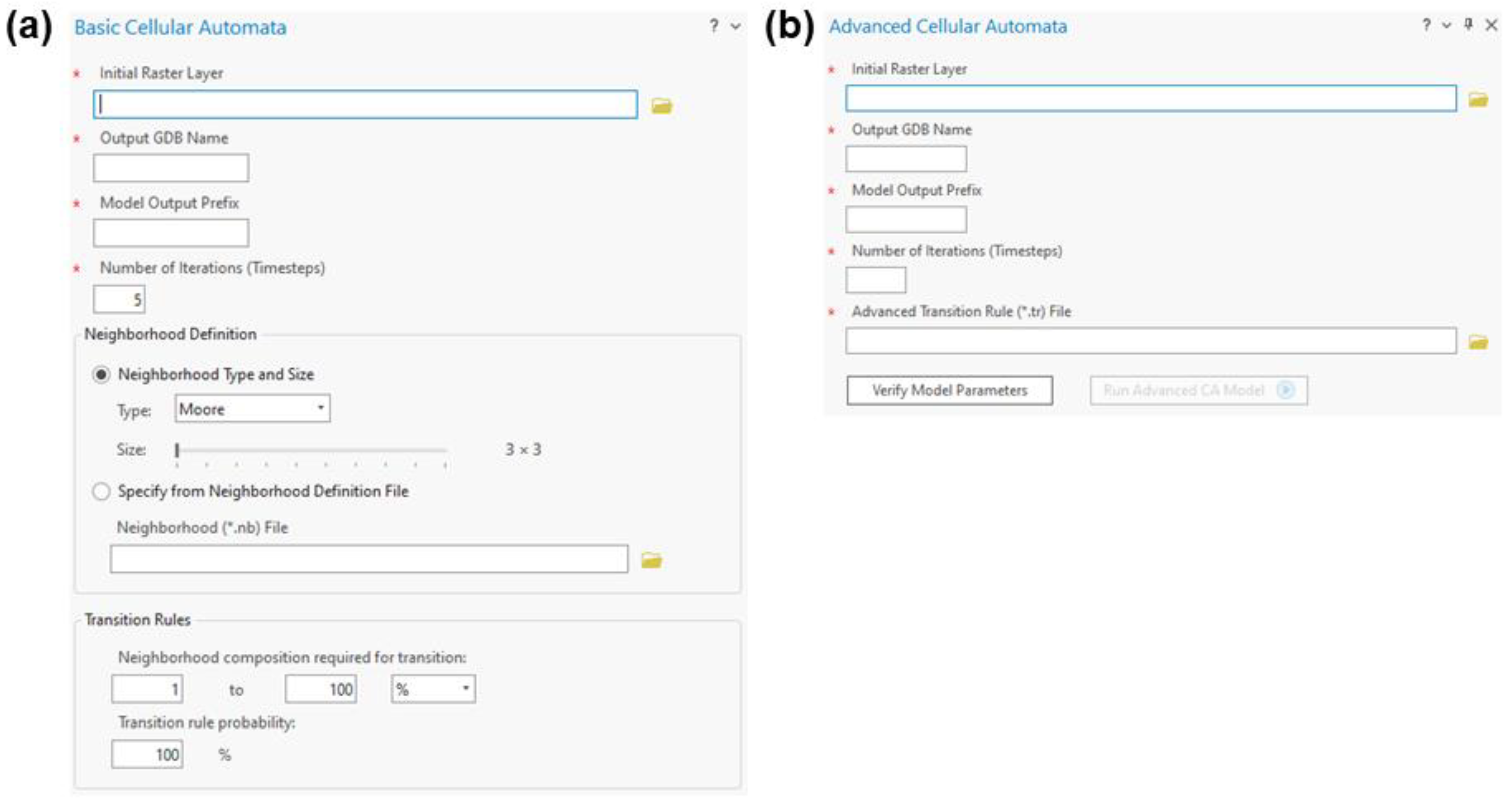
The Model Execution tool group contains the Basic CA and Advanced CA tools (Figure 6), with key differences outlined in Table 2. The Basic CA tool supports rapid implementation of binary models by including nested Model Parameterization functions within a single ArcGIS DockPane (Figure 6a). The Advanced CA tool supports binary or multi-class models, relying on a Transition Rule file to parameterize simple to complex model behaviors (Figure 6b). Each time a Basic or Advanced CA modeling tool is run, a Model Parameter Report is generated and saved to the output directory. The Model Parameter Report supports interpretation and communication of model behavior. The report includes information about model execution time, datasets used, output directory information, the number of timesteps, and a table of linguistic transition rule explanations that can be copied or modified for scientific communications.

3.2.2. Transition Rule Execution

Given that fully probabilistic framing often impedes model transparency given the manifold interpretations for why the pattern emerged [80], transition rules are applied as a series of basic IF–THEN conditions to maintain model explainability in support of real-world spatial planning and decision-making practices. With obvious computational costs, it is necessary to process subsets or “blocks” of raster layers in parallel, as articulated in previous work [81]. For Cell-Level, Allocation and Quantity, and Constraint rules, data subsets are easy to assign to worker threads because blocks do not require information about states of nearby locations. Conversely, Neighborhood-Based and Stochastic Disturbance rules with proximal or distance-based operations require overlapping subareas or block “halos” to be delegated to worker threads [82]. The default number of worker threads is currently limited to half the number of threads available on the computing hardware.

3.3. Model Evaluation

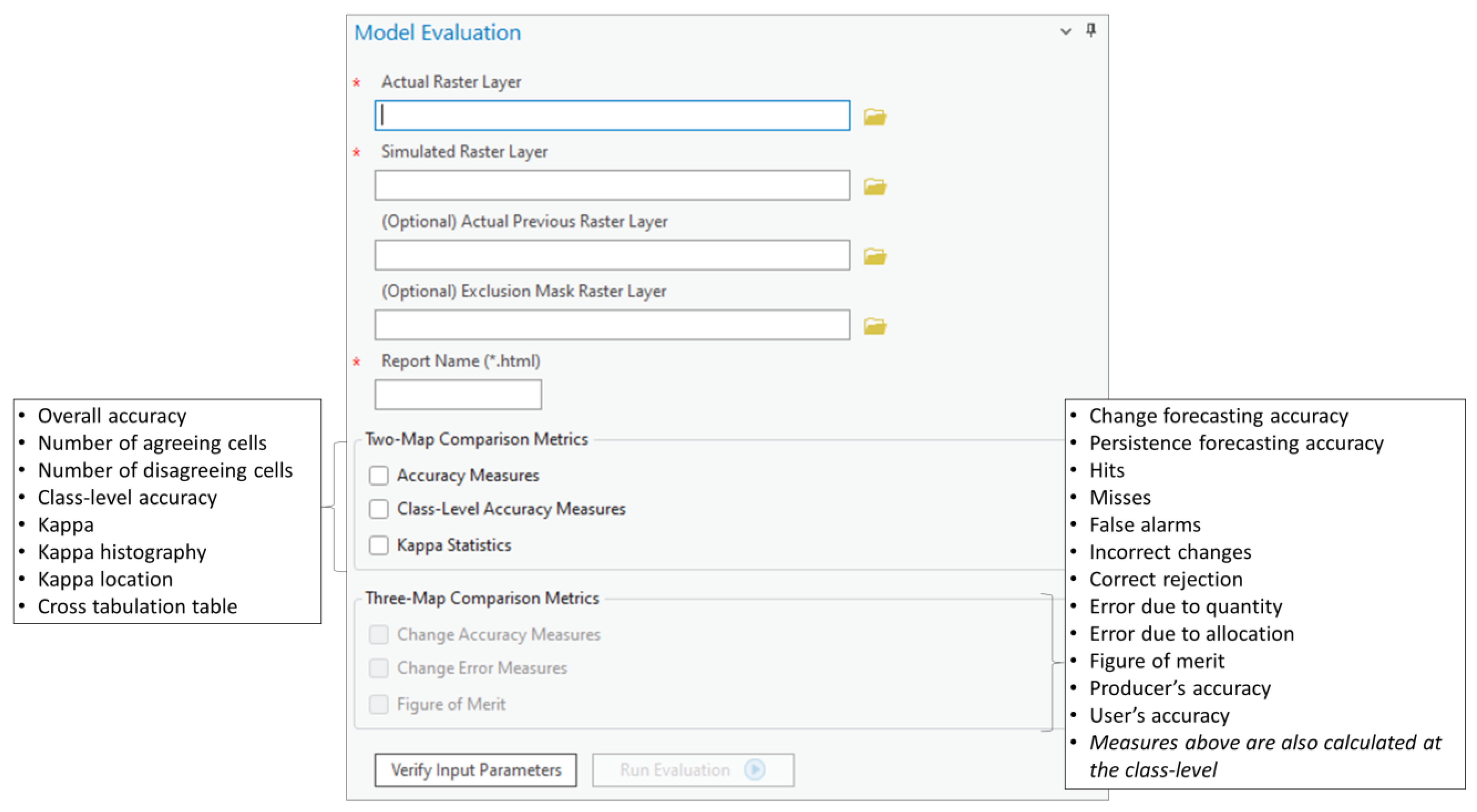
The Model Evaluation tool provides a selection of two- and three-map comparison metrics (Figure 7) and outputs an HTML file containing the calculated values. Two-map comparison measures are typically used to quantify the cell-by-cell agreement between a real and simulated map, while three-map comparisons emphasize agreement of changed locations [83]. In the Model Evaluation tool, two-map comparison metrics include overall accuracy measures [34], cross-tabulation matrices [84], disagreements of quantity and allocation [85], and Kappa statistics [86]. The three-map comparison metrics implemented include change error measures [87], figure of merit (FOM) [83], and class-level change metrics [88].

4. Implementing Models with the Geographic Automata Add-In: Two Case Studies

Two case studies are developed to demonstrate the functionality of the Geographic Automata add-in and its application for modeling real-world spatiotemporal phenomena. The first case study simulates forest insect infestation by drawing on documented behaviors to show how increasingly complex spatial patterns can be achieved with the five generic transition rule types explained in Section 3.1.2. The second case study simulates urban growth and compares traditional ML-CA outcomes with a novel AutoML-CA integration. Both case studies were executed on a PC running Windows 11 Pro and ArcGIS Pro version 3.2. The PC was equipped with an i7-13700K CPU, 64 GB of RAM, and an NVIDIA GTX 1080Ti GPU.

4.1. Case Study 1: Multi-Class CA Modeling of a Forest Insect Infestation

The purpose of this case study is to show how any number of rules of each rule type can be encoded and executed using the Advanced CA tool workflow from the Geographic Automata add-in. In this case study, five scenarios were developed to illustrate how increasingly complex behavior of forest insect infestation is realized with the generic transition rule types. That is, rule lists for each scenario show the effects of layering different transition rules and rule types to generate more realistic or nuanced outcomes. While the scenarios are hypothetical, they are implemented using real-world geospatial datasets related to a Mountain Pine Beetle (MPB) infestation. Transition rule mechanisms are based on previous CA models of MPB infestations [55,89], where changes are generated or limited based on neighborhood conditions, infilling settings, distance dispersal length, susceptibility maps, quantity limits, and spatial constraints.

4.1.1. Study Area and Datasets

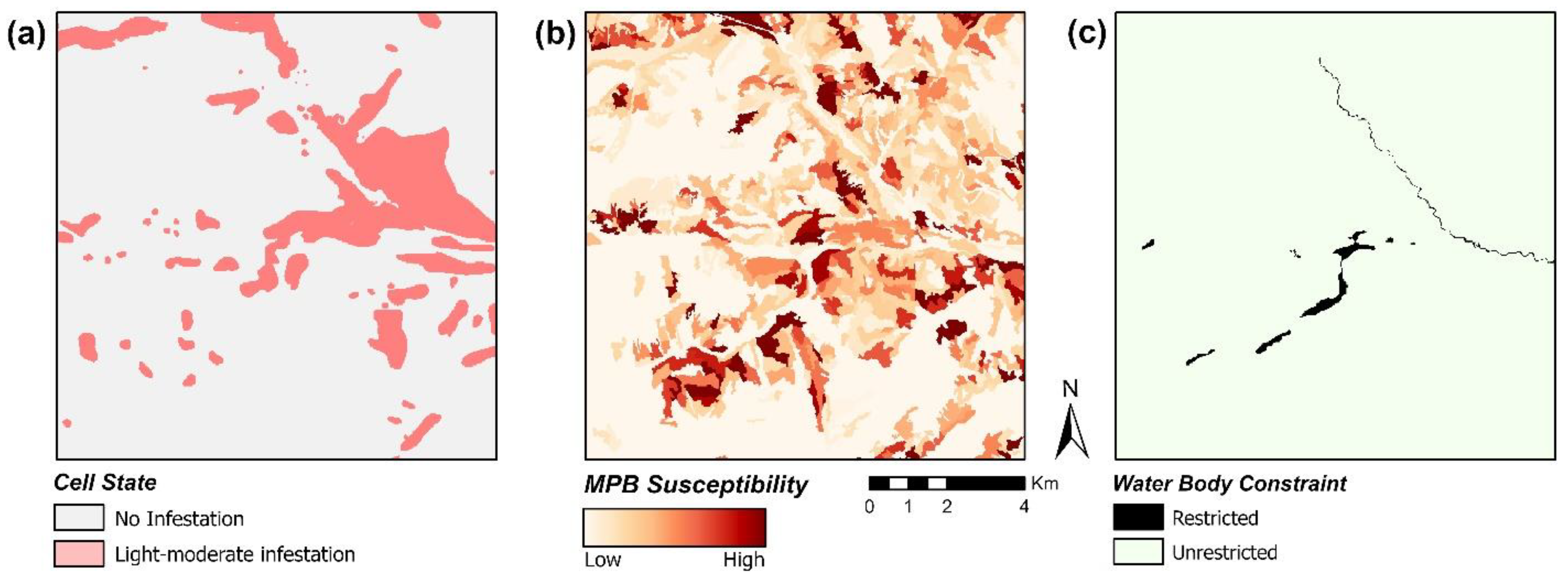
This case study focuses on a location spanning 130.29 km2 within Manning Provincial Park, situated in the Cascade Mountains of British Columbia, Canada. To initialize the model scenarios configured with the Geographic Automata add-in tooling, real-world datasets were acquired from the BC Data Catalogue [90]. These include an initial infestation map of the infested areas in 2004 [91], MPB susceptibility indices [92], and water bodies. The MPB susceptibility indices were obtained from the “Bark Beetle Susceptibility Rating” dataset [92], which contains hazard ratings derived from key factors including basal area, age, density, and location of pine trees. To prepare each dataset for this case study, each of the original vector datasets was clipped to the extent of the study region. Next, the vector datasets were rasterized to a 30 m spatial resolution, each with 384 rows and 377 columns (Figure 8). Maps are displayed with the NAD 1983 UTM Zone 10N projected coordinate system.

4.1.2. Model Implementation

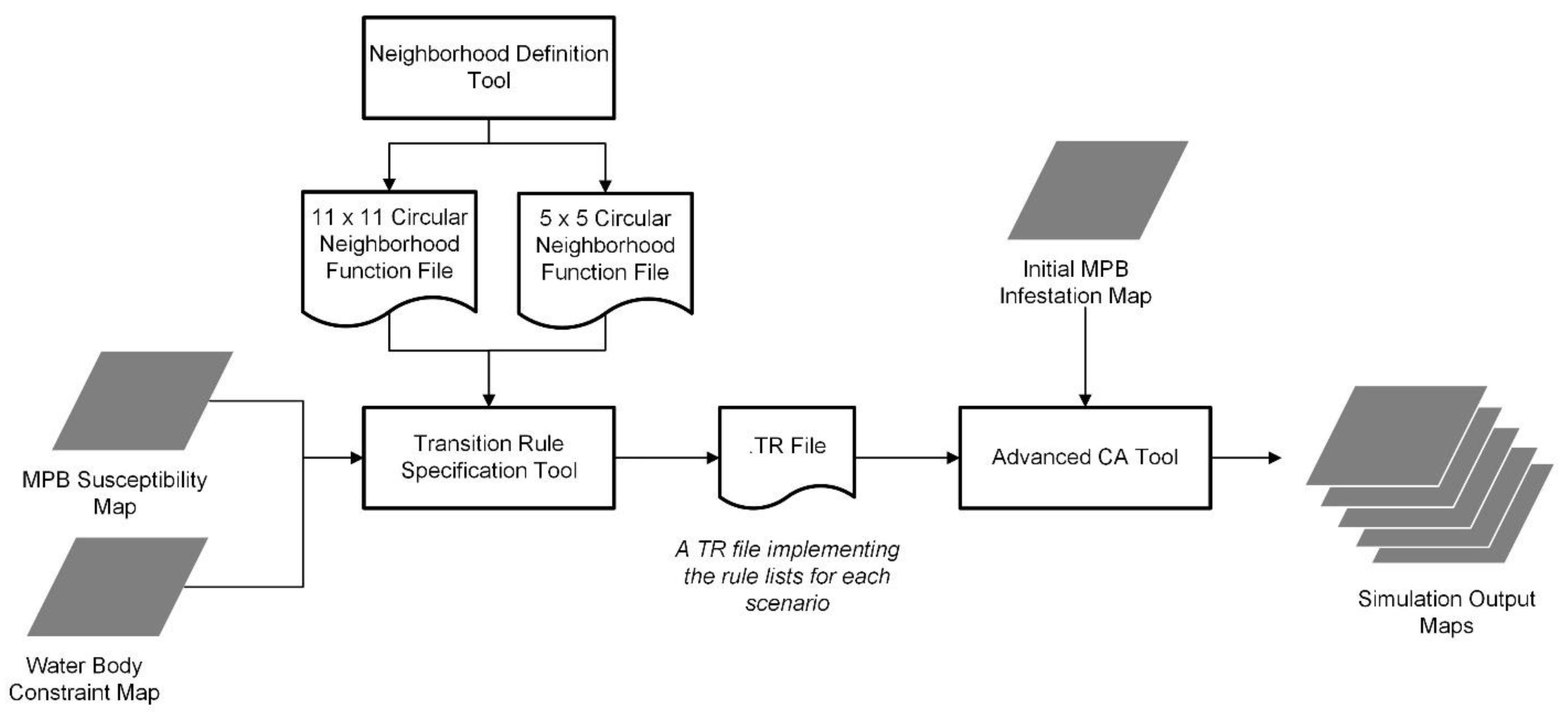
Five scenarios were parameterized and executed to generate outcomes using the procedure shown in Figure 9, which leverages the Neighborhood Definition, Transition Rule Specification, and Advanced CA tools.

Cell States

Three cell states are represented in the hypothetical models: (0) not infested, (1) light–moderate infestation, and (2) severe infestation (30% or more trees in the location recently killed) based on intensity classes from the aerial overview survey used to derive the initial data layer [91].

Scenario Setup and Transition Rules

The scenarios demonstrate increasing complexity of MPB infestation behavior encoded using one or several transition rule types. In this case study, each scenario expands on the rule set implemented in its predecessor. For example, the behavior portrayed in Scenario 1 is augmented in Scenario 2, and so forth. The transition rules and scenario settings are outlined in Table 3.

Model Execution

The Advanced CA tool is used to execute the infestation model with the MPB infestation data for 2004 (Figure 8a) provided as the initial raster layer. The number of iterations is set to five, where each iteration of the model represents one year of MPB dispersal.

4.1.3. Results

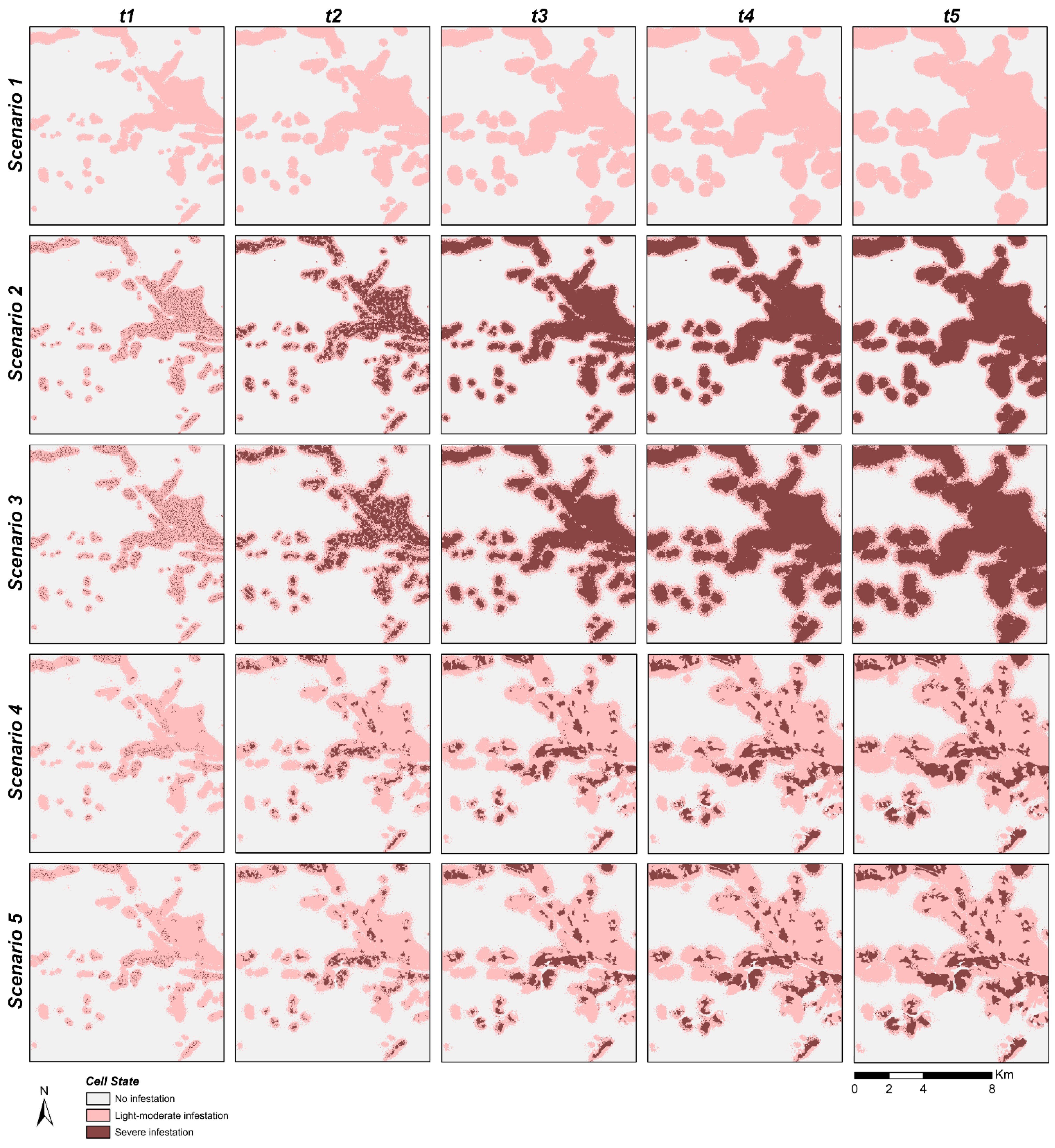
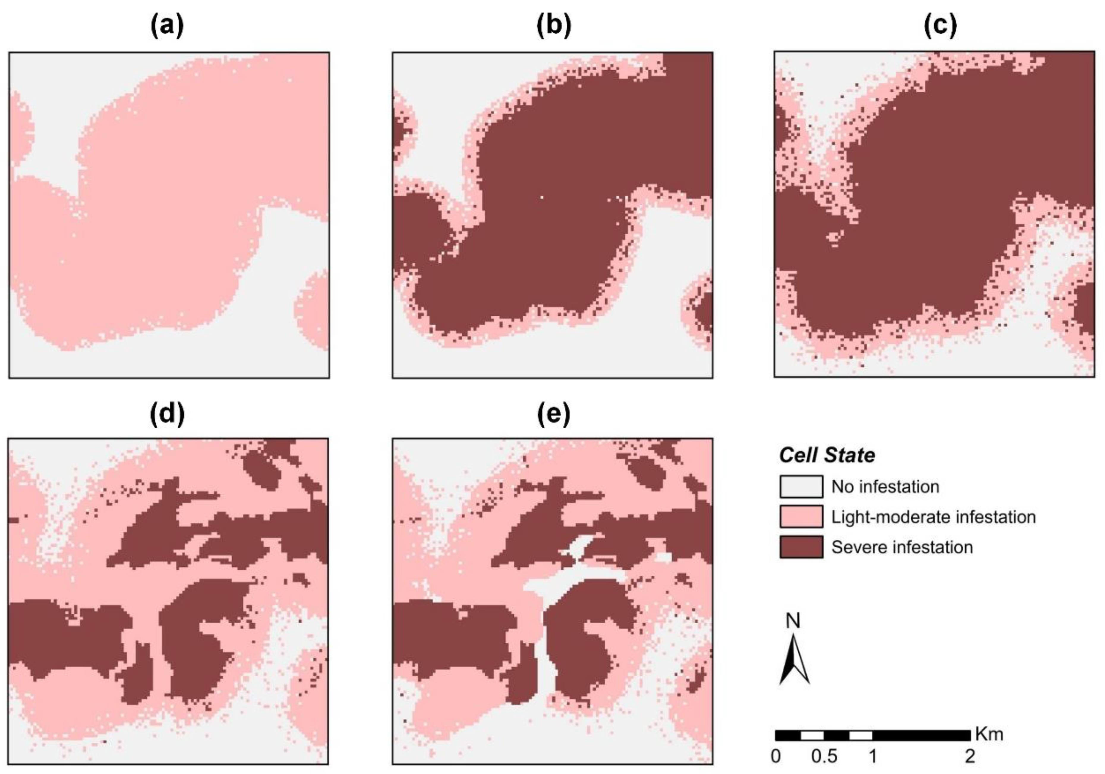
The model execution time for each scenario was 31 to 36 s. The respective outcomes are displayed in Figure 10. Rule types defining Scenarios 1 through 3 are exclusively generative, with hypothetical MPB dispersal and intensification propelled with Neighborhood-Based, Cell-Level, and Stochastic Disturbance rule types. Meanwhile, Scenarios 4 and 5 introduce limiting or refining mechanisms via the Allocation and Quantity and Constraint rules. The simulated outcomes for Scenarios 4 and 5 also present the capacity of the Geographic Automata add-in to incorporate auxiliary datasets like susceptibility maps and constraints during model execution. For instance, the insect infestation simulation outcomes of Scenario 5 are prevented from spreading to locations with water bodies or rivers (Figure 11e). After obtaining model outputs, other data layers pertaining to constraints or other relevant layers can be overlayed with simulation outcomes using ArcGIS Pro’s existing geoprocessing functions. Overall, the visual comparison shows how the Geographic Automata add-in can be used to model multi-class changes, to integrate real-world datasets, and to produce simple to complex spatial patterns of insect infestation through combining and layering rules created from the five basic rule types.

4.2. Case Study 2: Comparing ML-CA Models of Urban Growth

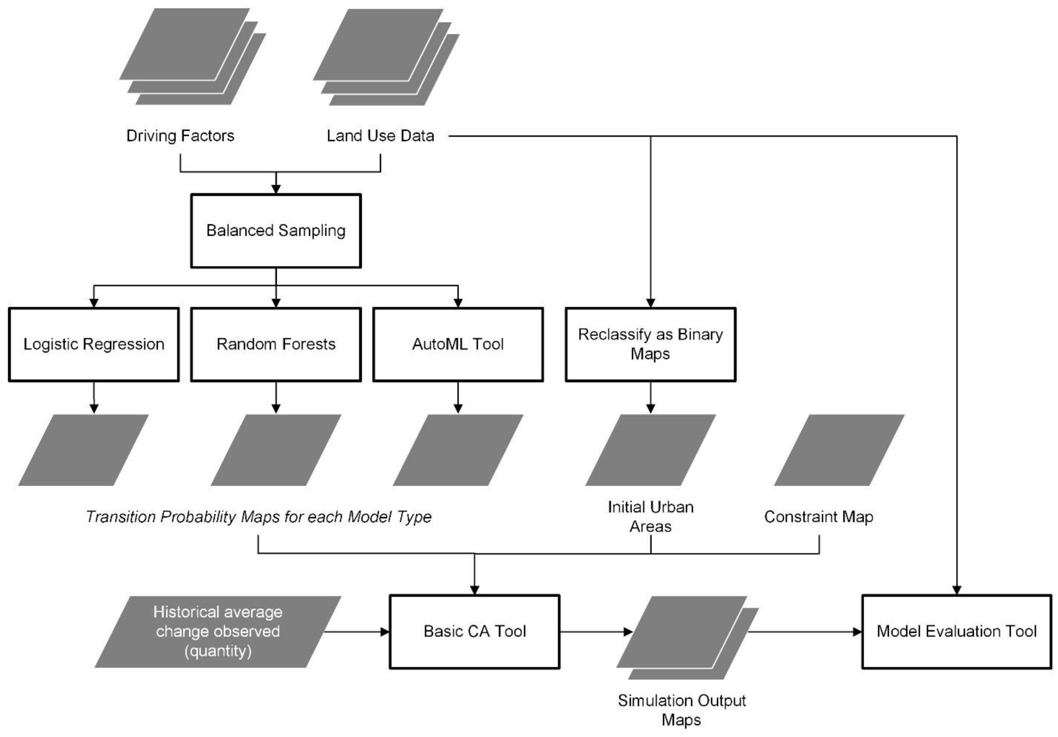
The second case study demonstrates a novel combination of ArcGIS Pro tools and Geographic Automata add-in functionality to execute a comparison of ML-CA models for simulating urban growth (Figure 12). This example compares the effects of using urban growth probabilities outputted by different ML models to inform CA transitions [4] including logistic regression (LR) [50,93] and random forests (RF) [4,38]. The traditional ML-CA approaches are compared with an inaugural implementation of automated machine learning (AutoML) with CA to guide new urban allocations. Although this abridged workflow does not delve into ML model validation, testing, and feature importance analysis details, such operations are possible in the ArcGIS Pro software.

4.2.1. Study Area and Datasets

This case study focuses on modeling urban developments in the Township of Langley, located in the rapidly growing Metro Vancouver Regional District of British Columbia, Canada. Land use datasets were obtained from Agriculture and Agri-Food Canada (AAFC) for years 2000 (T0), 2010 (T1), and 2020 (T2). The auxiliary data layers used as explanatory factors to train the ML models are listed in Table 4. All data processing procedures ensured layers were aligned to the 30 m spatial resolution of the AAFC Land Use datasets. The study area extent covers approximately 317.52 km2, with raster datasets spanning 541 rows and 775 columns to encapsulate the municipality extent. Maps are displayed with the NAD 1983 UTM Zone 10N projected coordinate system.

4.2.2. Model Implementation

Cell States

Binary cell states are specified as follows: (0) non-urban areas and (1) urban areas.

Training ML Models and Generating Change Probability Maps

For the ML subroutine, the training label is created by reclassifying the land use data for 2010 (T1) such that urban areas and non-urban areas are signified by ones and zeros, respectively. Next, the training dataset imbalance is addressed by retaining equal numbers of changed and persistent samples [73]. Of the 352,803 cells comprising the study area, 46,825 cells transitioned to urban between 2000 and 2010. To create the balanced dataset, all changed samples are included in the training dataset, while 46,825 persistent cells are randomly sampled from non-urban unchanged locations. The final training dataset contains 93,650 samples.
The LR and RF models are implemented in an ArcGIS Pro Notebook calling on scikitlearn functionality, while the ensemble model is executed using the graphical AutoML tool available in ArcGIS Pro’s GeoAI toolbox. All models are trained with 80% of the balanced training dataset, while 20% is withheld for ML validation purposes. Next, the LR, RF, and AutoML models are applied to estimate the urban development probability values across the study area.

Model Types and Transition Rule Specification

Four model types are configured using the Basic CA tool: LR-CA, RF-CA, AutoML-CA1, and AutoML-CA2. Each model type differs in the Allocation and Quantity rule implementation shown in Table 5. Additionally, the AutoML-CA2 configuration implements an alternative ML-CA model structure using demand limits instead of setting a minimum suitability value [94].

Model Execution

Using the Basic CA tool, the initial raster layer represents urban areas in the year 2000 (T0). The number of timesteps is set to two, where one iteration represents a 10-year temporal interval. The actual datasets for T1 and T2 are used for CA model calibration and validation, respectively.

Model Evaluation

In CA model calibration, the goal is to adjust model parameters to reduce differences between simulated outcomes and observed data. In model validation, simulated outcomes are compared to real-world data independent from model calibration. Using the Model Evaluation tool, agreement of real and simulated maps is quantified for calibration and validation stages. To calibrate the model in this case study, the FOM value is primarily used to determine agreement of changed locations. This three-map comparison measure requires an initial raster layer, a reference layer, and a simulated layer. Therefore, the tool inputs include the urban areas in the year 2000 as the initial raster layer, the real urban areas in the year 2010 as the reference layer, and first timestep outputted by the model as the simulated layer. To calculate metrics for the validation stage, the initial raster is maintained, while the reference layer is replaced with the layer depicting urban areas in the year 2020 and the simulated layer is the second timestep generated by the model. Cells outside of the township boundary are excluded to ensure the model evaluation results are not obscured. The options selected in the Model Evaluation tool were Accuracy Measures, Kappa Statistics, Change Error Assessment, and Figure of Merit from the GUI options presented in Figure 7.

4.2.3. Results

The Basic CA model execution time was 12, 10, 10, and 30 s for each model type, respectively. The simulated outcomes for years 2010 and 2020 produced by each model configuration are shown in Figure 13, and corresponding metrics obtained from the Model Evaluation tool are presented in Table 6.
In both calibration and validation metrics (Table 6), there is a general upward trend observed from the LR-CA to AutoML-CA2 models. The LR-CA models are associated with the lowest overall accuracy, Kappa, and FOM values for both calibration and validation stages, which adheres to comparative findings reported in other studies [38,50]. This model also produced the most “false alarms”, meaning that there were more new developments forecasted to actual undeveloped locations than the other model types (Figure 14). Measures of agreement and error associated with RF-CA and AutoML-CA1 model outcomes are most similar. Meanwhile, the overall accuracy and Kappa measures related to AutoML-CA2 suggest the quantity limit imposed in Rule D (Table 5) helped to reduce false alarms, which is confirmed in the Change Error Assessment measures graphed in Figure 14. Overall, this abridged ML-CA model comparison showed how real end-to-end model-building procedures can be conducted using a combination of the Geographic Automata add-in and ArcGIS Pro functionality. Once the stages of CA model calibration and validation are completed, the best performing ML-CA model can be used to project urban growth for more iterations to obtain simulated maps of years 2030, 2040, and beyond. In addition, the model can be adapted to explore possible scenarios such as simulating faster or slower urban expansion based on population projections or examining the effects of new forest conservation or urban densification policies for the municipality.

5. Discussion

This study introduces the first version of the Geographic Automata add-in for ArcGIS Pro. The add-in was developed to address the lack of general-purpose GUI-based CA technologies available in contemporary GIS software. Two case studies illustrated how the add-in (1) provides general-purpose functions capable of supporting binary or multi-class CA models of various geospatial systems and (2) facilitates end-to-end model-building activities that can be intertwined with ArcGIS Pro functionality.
In the first case study, five MPB infestation scenarios presented the incremental effects of combining and layering different transition rule types to implement a multi-class CA model. The various scenario settings show the capabilities of the add-in tools to support as many generative or limiting rules as a user decides. For instance, each scenario applied additional rule mechanisms that produced increasingly complex spatial patterns. The outcomes demonstrate the flexibility of transition rule types for use with real-world geospatial datasets and for capturing the characteristics of documented insect infestation behavior. For example, Scenario 3 showed a possible integration of behaviors drawn from previous studies, while Scenarios 4 and 5 exemplified how dispersal could be guided with an expert-derived susceptibility map and real-world physical constraints. Although some previous studies describing CA models of MPB infestation have excluded detailed information about the software or programming required to implement model behaviors described [55], the Geographic Automata add-in tools enable researchers to encode documented dispersal mechanisms or investigate other possible processes that propel changes observed over space and time.
The second case study demonstrates an end-to-end model-building activity involving built-in ArcGIS Pro functionality and Geographic Automata add-in tooling to compare the effects of ML-generated transition potential maps on CA model outcomes. The comparison centered on comparing urban growth forecasts of traditional ML-CA models with those produced by a novel AutoML-CA approach. The simulated outputs of each model type adhered to trends reported in scientific literature using ML-CA routines [38,50]. However, both studies relied on patchworks of software and custom programmed functionality to implement and execute ML-CA routines. For example, Kamusoko and Gamba [38] relied on an assortment of tools including Esri’s ArcMap, the Dinamica EGO software, various ML packages available in R, and the Map Comparison Kit. The methodology presented by Shafizadeh-Moghadam et al. [50] similarly included ArcMap, a standalone NN-based land transformation modeling tool, and other ML models coded with MATLAB, R, and Java. In contrast to the mosaics of disparate tooling described in preceding studies, the second case study demonstrates the capacity of the Geographic Automata add-in to support a simple, streamlined model-building workflow within an established GIS software. The presented workflow shows the capability of the Geographic Automata add-in tools to support researchers in implementing rapid comparisons of CA models enhanced with outcomes of other analyses.
At this point, there are numerous possible trajectories for enhancing and extending the inaugural version of the Geographic Automata add-in. Several enhancements of existing CA functionality could include adding a transition rule fallback routine, implementing support for dynamic variables and rule applications at specific temporal intervals, adding explicit distance decay or weighted neighborhood function options, conducting more rigorous performance benchmarking, expanding model parameter reports and rule tracing options, and improving UI components. As tool development progresses, so should a library of technical resources such as video tutorials and documentation web pages for researchers, educators, and students. Next, the Model Evaluation tool would benefit from an expanded assortment of metrics to support researchers looking to examine different aspects of model outcomes [36]. Possible additions may include Fuzzy Kappa, the Total Operating Characteristic (TOC), or landscape metrics. Another avenue for future upgrades is to emphasize and expand on existing functionality to facilitate explainable CA models. Currently, a potentially debatable but deliberate restriction of this work is that transition rule mechanisms cannot be replaced fully with black-box sub-models. If explainable outcomes are not required, users can use Allocation and Quantity rules to incorporate the outcomes of any statistical analysis technique in their CA model implementation, as demonstrated in the second case study. Lastly, the Geographic Automata add-in naming was intentional and preserves opportunities to extend CA modeling capabilities and to support other GA models. For example, functionality can be expanded to provide generalized functions for implementing ABMs and hybrid ABM-CA models in ArcGIS Pro to further advance geospatial technologies designed for geosimulation.

6. Conclusions

This paper introduces the Geographic Automata add-in created for ArcGIS Pro 3.1 and newer. Despite the theoretical simplicity of CA, those looking to implement models without specialized, inflexible, or black-box embellishments must have programming skills, rely on ad hoc procedures spanning numerous GUI-based software tools, or leverage a mixture of both. To address the absence of geospatial technologies available for streamlining CA model-building activities, the Geographic Automata add-in provides general-purpose functionality demonstrably capable of supporting CA model implementations of various geospatial phenomena. The add-in also maintains direct connections between general GAS and CA model theory and implementation, supporting users of all skill levels to transfer proficiencies more easily to new domains or tooling. These qualities can facilitate the add-in’s usage for educational purposes and facilitate hands-on learning experiences in classroom settings. Likewise, the add-in serves as a launch point for researchers and decision-makers looking to survey methodologies, conduct model comparisons, and implement integrations of CA with different analysis procedures available in ArcGIS Pro.
In summary, the Geographic Automata add-in provides a first step toward generic, user-friendly CA model-building tools accessible in the ArcGIS Pro software environment. Its functionality supports a wide range of users such as researchers, educators, and decision-makers. Future upgrades intend to enhance transparency and expand utility of the add-in for research, education, and real-world spatial decision-making settings.

Author Contributions

Conceptualization, Formal analysis, Investigation, Methodology, Writing—original draft, Writing—review and editing, A.v.D. and S.D.; Funding acquisition, Supervision, S.D.; Software, A.v.D. All authors have read and agreed to the published version of the manuscript.

Funding

This research was funded by the Natural Sciences and Engineering Research Council (NSERC) of Canada through the Discovery Grant [RGPIN-2023-04052] awarded to the second author.

Institutional Review Board Statement

Not applicable.

Informed Consent Statement

Not applicable.

Data Availability Statement

Publicly available datasets are used for each case study described in Section 4. For case study 1, MPB infestation polygons, susceptibility indices, and water bodies were obtained from the BC Data Catalog https://catalogue.data.gov.bc.ca/ (accessed 7 November 2023). In case study 2, data layers are derived from the Agriculture and Agri-Food Canada (AAFC) Land Use dataset https://open.canada.ca/data/en/dataset/fa84a70f-03ad-4946-b0f8-a3b481dd5248 (accessed 7 November 2023), the ASTER Digital Elevation Model https://asterweb.jpl.nasa.gov/gdem.asp (accessed 7 November 2023), the BC Data Catalog https://catalogue.data.gov.bc.ca/ (accessed 7 November 2023), the Township of Langley Open Data Portal https://data-tol.opendata.arcgis.com/ (accessed 7 November 2023), and the Government of Canada Open Data Portal.https://open.canada.ca/data/en/dataset/4f154582-bc36-42fb-8dee-25d863466081 (accessed 7 November 2023).

Acknowledgments

We are thankful for the full support of this research work by the Natural Sciences and Engineering Research Council (NSERC) of Canada. We also greatly appreciate the positive and constructive feedback provided by the anonymous reviewers and the journal Academic Editor. Furthermore, we extend our gratitude to the Product and SDK engineers from Esri Inc. for answering our questions related to the ArcGIS Pro SDK for .NET.

Conflicts of Interest

The authors declare no conflicts of interest.

Software Availability Statement

The Geographic Automata add-in is available for ArcGIS Pro 3.1 and newer. It can be downloaded for from ArcGIS Online (https://arcg.is/1feLKP (accessed on 20 July 2024)).

References

  1. Torrens, P.M.; Benenson, I. Geographic Automata Systems. Int. J. Geogr. Inf. Sci. 2005, 19, 385–412. [Google Scholar] [CrossRef]
  2. Wu, X.; Dong, W.; Wu, L.; Liu, Y. Research Themes of Geographical Information Science during 1991–2020: A Retrospective Bibliometric Analysis. Int. J. Geogr. Inf. Sci. 2022, 37, 243–275. [Google Scholar] [CrossRef]
  3. Batty, M.; Xie, Y. From Cells to Cities. Environ. Plan. B Plan. Des. 1994, 21, 531–548. [Google Scholar] [CrossRef]
  4. Rienow, A.; Mustafa, A.; Krelaus, L.; Lindner, C. Modeling Urban Regions: Comparing Random Forest and Support Vector Machines for Cellular Automata. Trans. GIS 2021, 25, 1625–1645. [Google Scholar] [CrossRef]
  5. Santé, I.; García, A.M.; Miranda, D.; Crecente, R. Cellular Automata Models for the Simulation of Real-World Urban Processes: A Review and Analysis. Landsc. Urban. Plan. 2010, 96, 108–122. [Google Scholar] [CrossRef]
  6. Von Neumann, J. Theory of Self-Reproducing Automata; Burks, A.W., Ed.; University of Illinois Press: Champaign, IL, USA, 1966. [Google Scholar]
  7. Wolfram, S. Cellular Automata as Models of Complexity. Nature 1984, 311, 419–424. [Google Scholar] [CrossRef]
  8. Torrens, P.M. Cellular Automata. In International Encyclopedia of Human Geography, 1st ed.; Thrift, N., Kitchin, R., Eds.; Elsevier Science: London, UK, 2009; pp. 1–4. ISBN 9780080449104. [Google Scholar]
  9. Batty, M.; Couclelis, H.; Eichen, M. Urban Systems as Cellular Automata. Environ. Plan. B Plan. Des. 1997, 24, 159–164. [Google Scholar] [CrossRef]
  10. Itami, R.M. Simulating Spatial Dynamics: Cellular Automata Theory. Landsc. Urban. Plan. 1994, 30, 27–47. [Google Scholar] [CrossRef]
  11. Xie, Y. A Generalized Model for Cellular Urban Dynamics. Geogr. Anal. 1996, 28, 350–373. [Google Scholar] [CrossRef]
  12. Batty, M.; Torrens, P.M. Modelling and Prediction in a Complex World. Futures 2005, 37, 745–766. [Google Scholar] [CrossRef]
  13. Wu, F. A Linguistic Cellular Automata Simulation Approach for Sustainable Land Development in a Fast Growing Region. Comput. Environ. Urban. Syst. 1996, 20, 367–387. [Google Scholar] [CrossRef]
  14. Zhang, D.; Liu, X.; Lin, Z.; Zhang, X.; Zhang, H. The Delineation of Urban Growth Boundaries in Complex Ecological Environment Areas by Using Cellular Automata and a Dual-Environmental Evaluation. J. Clean. Prod. 2020, 256, 120361. [Google Scholar] [CrossRef]
  15. Wen, R.; Li, S. Spatial Decision Support Systems with Automated Machine Learning: A Review. ISPRS Int. J. Geoinf. 2023, 12, 12. [Google Scholar] [CrossRef]
  16. Li, X.; Yeh, A.G.O. Zoning Land for Agricultural Protection by the Integration of Remote Sensing, GIS, and Cellular Automata. Photogramm. Eng. Remote Sens. 2001, 67, 471–477. [Google Scholar]
  17. White, R.; Engelen, G. High-Resolution Integrated Modelling of the Spatial Dynamics of Urban and Regional Systems. Comput. Environ. Urban. Syst. 2000, 24, 383–400. [Google Scholar] [CrossRef]
  18. Liu, M.; Chen, H.; Qi, L.; Chen, C. LUCC Simulation Based on RF-CNN-LSTM-CA Model with High-Quality Seed Selection Iterative Algorithm. Appl. Sci. 2023, 13, 3407. [Google Scholar] [CrossRef]
  19. Aburas, M.M.; Ho, Y.M.; Ramli, M.F.; Ash’aari, Z.H. The Simulation and Prediction of Spatio-Temporal Urban Growth Trends Using Cellular Automata Models: A Review. Int. J. Appl. Earth Obs. Geoinf. 2016, 52, 380–389. [Google Scholar] [CrossRef]
  20. Liu, M.; Liao, X.; Chen, C. Urbanization Process: A Simulation Method of Urban Expansion Based on RF-SNSCNN-CA Model. Appl. Sci. 2023, 13, 6615. [Google Scholar] [CrossRef]
  21. Kyriakou, C.; Georgoudas, I.G.; Papanikolaou, N.P.; Sirakoulis, G.C. A GIS-Aided Cellular Automata System for Monitoring and Estimating Graph-Based Spread of Epidemics. Nat. Comput. 2022, 21, 463–480. [Google Scholar] [CrossRef]
  22. Addae, B.; Dragićević, S. Modelling Global Deforestation Using Spherical Geographic Automata Approach. ISPRS Int. J. Geoinf. 2023, 12, 306. [Google Scholar] [CrossRef]
  23. Alexandridis, A.; Vakalis, D.; Siettos, C.I.; Bafas, G.V. A Cellular Automata Model for Forest Fire Spread Prediction: The Case of the Wildfire That Swept through Spetses Island in 1990. Appl. Math. Comput. 2008, 204, 191–201. [Google Scholar] [CrossRef]
  24. Bone, C.; Dragicevic, S.; Roberts, A. A Fuzzy-Constrained Cellular Automata Model of Forest Insect Infestations. Ecol. Model. 2006, 192, 107–125. [Google Scholar] [CrossRef]
  25. Perez, L.; Dragicevic, S. Landscape-Level Simulation of Forest Insect Disturbance: Coupling Swarm Intelligent Agents with GIS-Based Cellular Automata Model. Ecol. Model. 2012, 231, 53–64. [Google Scholar] [CrossRef]
  26. Pardo-Igúzquiza, E.; Collados-Lara, A.J.; Pulido-Velazquez, D. Estimation of the Spatiotemporal Dynamics of Snow Covered Area by Using Cellular Automata Models. J. Hydrol. 2017, 550, 230–238. [Google Scholar] [CrossRef]
  27. Georgoudas, I.G.; Sirakoulis, G.C.; Scordilis, E.M.; Andreadis, I. A Cellular Automaton Simulation Tool for Modelling Seismicity in the Region of Xanthi. Environ. Model. Softw. 2007, 22, 1455–1464. [Google Scholar] [CrossRef]
  28. Barchyn, T.E.; Hugenholtz, C.H. A New Tool for Modeling Dune Field Evolution Based on an Accessible, GUI Version of the Werner Dune Model. Geomorphology 2012, 138, 415–419. [Google Scholar] [CrossRef]
  29. Fonseca, P.; Colls, M.; Casanovas, J. A Novel Model to Predict a Slab Avalanche Configuration Using m:N-CAk Cellular Automata. Comput. Environ. Urban. Syst. 2011, 35, 12–24. [Google Scholar] [CrossRef]
  30. Clarke, K.C.; Hoppen, S.; Gaydos, L. A Self-Modifying Cellular Automaton Model of Historical Urbanization in the San Francisco Bay Area. Environ. Plan. B Plan. Des. 1997, 24, 247–261. [Google Scholar] [CrossRef]
  31. Batty, M.; Xie, Y.; Sun, Z. Modeling Urban Dynamics through GIS-Based Cellular Automata. Comput. Environ. Urban. Syst. 1999, 23, 205–233. [Google Scholar] [CrossRef]
  32. Waddell, P. Urbansim: Modeling Urban Development for Land Use, Transportation, and Environmental Planning. J. Am. Plan. Assoc. 2002, 68, 297–314. [Google Scholar] [CrossRef]
  33. Van Delden, H.; Escudero, J.C.; Uljee, I.; Engelen, G. METRONAMICA: A Dynamic Spatial Land Use Model Applied to Vitoria-Gasteiz. In Virtual Seminar of the MILES Project; Centro de Estudios Ambientales: Vitoria-Gasteiz, Spain, 2005; pp. 1–8. [Google Scholar]
  34. Liu, X.; Liang, X.; Li, X.; Xu, X.; Ou, J.; Chen, Y.; Li, S.; Wang, S.; Pei, F. A Future Land Use Simulation Model (FLUS) for Simulating Multiple Land Use Scenarios by Coupling Human and Natural Effects. Landsc. Urban. Plan. 2017, 168, 94–116. [Google Scholar] [CrossRef]
  35. Stevens, D.; Dragicevic, S.; Rothley, K. ICity: A GIS-CA Modelling Tool for Urban Planning and Decision Making. Environ. Model. Softw. 2007, 22, 761–773. [Google Scholar] [CrossRef]
  36. Cuellar, Y.; Perez, L. Assessing the Accuracy of Sensitivity Analysis: An Application for a Cellular Automata Model of Bogota’s Urban Wetland Changes. Geocarto Int. 2023, 38, 2186491. [Google Scholar] [CrossRef]
  37. Gounaridis, D.; Chorianopoulos, I.; Symeonakis, E.; Koukoulas, S. A Random Forest-Cellular Automata Modelling Approach to Explore Future Land Use/Cover Change in Attica (Greece), under Different Socio-Economic Realities and Scales. Sci. Total Environ. 2019, 646, 320–335. [Google Scholar] [CrossRef] [PubMed]
  38. Kamusoko, C.; Gamba, J. Simulating Urban Growth Using a Random Forest-Cellular Automata (RF-CA) Model. ISPRS Int. J. Geoinf. 2015, 4, 447–470. [Google Scholar] [CrossRef]
  39. Wu, F. SimLand: A Prototype to Simulate Land Conversion through the Integrated GIS and CA with AHP-Derived Transition Rules. Int. J. Geogr. Inf. Sci. 1998, 12, 63–82. [Google Scholar] [CrossRef]
  40. Li, X.; Chen, Y.; Liu, X.; Li, D.; He, J. Concepts, Methodologies, and Tools of an Integrated Geographical Simulation and Optimization System. Int. J. Geogr. Inf. Sci. 2011, 25, 633–655. [Google Scholar] [CrossRef]
  41. Kocabas, V.; Dragicevic, S. Enhancing a GIS Cellular Automata Model of Land Use Change: Bayesian Networks, Influence Diagrams and Causality. Trans. GIS 2007, 11, 681–702. [Google Scholar] [CrossRef]
  42. Yassemi, S.; Dragićević, S.; Schmidt, M. Design and Implementation of an Integrated GIS-Based Cellular Automata Model to Characterize Forest Fire Behaviour. Ecol. Model. 2008, 210, 71–84. [Google Scholar] [CrossRef]
  43. Asia Air Survey; NextGIS. MOLUSCE: Modules for Land Use Change Evaluation. 2014. Available online: https://github.com/nextgis/qgis_molusce (accessed on 10 July 2024).
  44. Breckling, B.; Pe’er, G.; Matsinos, Y.G. Cellular Automata in Ecological Modelling. In Modelling Complex Ecological Dynamics: An Introduction into Ecological Modelling for Students, Teachers & Scientists; Springer Science & Business Media: Berlin/Heidelberg, Germany, 2011; pp. 105–117. ISBN 9783642050282. [Google Scholar]
  45. Soares, B.S.; Cerqueira, G.C.; Pennachin, C.L. DINAMICA—A Stochastic Cellular Automata Model Designed to Simulate the Landscape Dynamics in an Amazonian Colonization Frontier. Ecol. Model. 2002, 154, 217–235. [Google Scholar] [CrossRef]
  46. White, R.; Engelen, G. Cellular Automata and Fractal Urban Form: A Cellular Modelling Approach to the Evolution of Urban Land-Use Patterns. Environ. Plan. A 1993, 25, 1175–1199. [Google Scholar] [CrossRef]
  47. Park, S.; Wagner, D.F. Incorporating Cellular Automata Simulators as Analytical Engines in GIS. Trans. GIS 1997, 2, 213–231. [Google Scholar] [CrossRef]
  48. Wu, F.; Webster, C.J. Simulation of Land Development through the Integration of Cellular Automata and Multicriteria Evaluation. Environ. Plan. B Plan. Des. 1998, 25, 103–126. [Google Scholar] [CrossRef]
  49. Lai, T.; Dragićević, S.; Schmidt, M. Integration of Multicriteria Evaluation and Cellular Automata Methods for Landslide Simulation Modelling. Geomat. Nat. Hazards Risk 2013, 4, 355–375. [Google Scholar] [CrossRef]
  50. Shafizadeh-Moghadam, H.; Asghari, A.; Tayyebi, A.; Taleai, M. Coupling Machine Learning, Tree-Based and Statistical Models with Cellular Automata to Simulate Urban Growth. Comput. Environ. Urban. Syst. 2017, 64, 297–308. [Google Scholar] [CrossRef]
  51. Gao, C.; Feng, Y.; Tong, X.; Lei, Z.; Chen, S.; Zhai, S. Modeling Urban Growth Using Spatially Heterogeneous Cellular Automata Models: Comparison of Spatial Lag, Spatial Error and GWR. Comput. Environ. Urban. Syst. 2020, 81, 101459. [Google Scholar] [CrossRef]
  52. Li, X.; Yeh, A.G.O. Neural-Network-Based Cellular Automata for Simulating Multiple Land Use Changes Using GIS. Int. J. Geogr. Inf. Sci. 2002, 16, 323–343. [Google Scholar] [CrossRef]
  53. Ménard, A.; Marceau, D.J. Exploration of Spatial Scale Sensitivity in Geographic Cellular Automata. Environ. Plan. B Plan. Des. 2005, 32, 693–714. [Google Scholar] [CrossRef]
  54. Verstegen, J.A.; Karssenberg, D.; van der Hilst, F.; Faaij, A.P.C. Identifying a Land Use Change Cellular Automaton by Bayesian Data Assimilation. Environ. Model. Softw. 2014, 53, 121–136. [Google Scholar] [CrossRef]
  55. Liang, L.; Li, X.; Huang, Y.; Qin, Y.; Huang, H. Integrating Remote Sensing, GIS and Dynamic Models for Landscape-Level Simulation of Forest Insect Disturbance. Ecol. Model. 2017, 354, 1–10. [Google Scholar] [CrossRef]
  56. Olmedo, M.T.C.; Paegelow, M.; Mas, J.F.; Escobar, F. The Simulation Stage in LUCC Modeling. In Geomatic Approaches for Modeling Land Change Scenarios; Springer: Berlin/Heidelberg, Germany, 2018; pp. 27–51. ISBN 9783319608013. [Google Scholar]
  57. Moreno, N.; Ablan, M.; Tonella, G. SpaSim: A Software to Simulate Cellular Automata Models. In Proceedings of the 1st International Congress on Environmental Modelling and Software, Lugano, Switzerland, 24–27 June 2002; pp. 348–353. [Google Scholar]
  58. Clark Labs. TerrSet 2020 Geospatial Monitoring and Modeling Software. Available online: https://clarklabs.org/terrset/ (accessed on 10 July 2024).
  59. Viana, C.M.; Pontius, R.G.; Rocha, J. Four Fundamental Questions to Evaluate Land Change Models with an Illustration of a Cellular Automata–Markov Model. Ann. Am. Assoc. Geogr. 2023, 113, 2497–2511. [Google Scholar] [CrossRef]
  60. Anderson, T.; Dragicevic, S. A Geosimulation Approach for Data Scarce Environments: Modeling Dynamics of Forest Insect Infestation across Different Landscapes. ISPRS Int. J. Geoinf. 2016, 5, 9. [Google Scholar] [CrossRef]
  61. Ornstein, A. The Frequency of Hands-on Experimentation and Student Attitudes toward Science: A Statistically Significant Relation (2005-51-Ornstein). J. Sci. Educ. Technol. 2006, 15, 285–297. [Google Scholar] [CrossRef]
  62. Wagner, D.F. Cellular Automata and Geographic Information Systems. Environ. Plan. B Plan. Des. 1997, 24, 219–234. [Google Scholar] [CrossRef]
  63. Stevens, D.; Dragićević, S. A GIS-Based Irregular Cellular Automata Model of Land-Use Change. Environ. Plan. B Plan. Des. 2007, 34, 708–724. [Google Scholar] [CrossRef]
  64. Couclelis, H. From Cellular Automata to Urban Models: New Principles for Model Development and Implementation. Environ. Plan. B Plan. Des. 1997, 24, 165–174. [Google Scholar] [CrossRef]
  65. Jakeman, A.J.; Letcher, R.A.; Norton, J.P. Ten Iterative Steps in Development and Evaluation of Environmental Models. Environ. Model. Softw. 2006, 21, 602–614. [Google Scholar] [CrossRef]
  66. Microsoft C# Language Documentation. Available online: https://learn.microsoft.com/en-us/dotnet/csharp/ (accessed on 21 April 2024).
  67. Esri ArcGIS Pro SDK for .NET. Available online: https://developers.arcgis.com/documentation/arcgis-add-ins-and-automation/arcgis-pro/ (accessed on 8 January 2024).
  68. Costanza, R.; Wainger, L.; Folke, C. Modeling Complex Ecological Economic Systems. Bioscience 1993, 43, 545–555. [Google Scholar] [CrossRef]
  69. Wu, H.; Zhou, L.; Chi, X.; Li, Y.; Sun, Y. Quantifying and Analyzing Neighborhood Configuration Characteristics to Cellular Automata for Land Use Simulation Considering Data Source Error. Earth Sci. Inform. 2012, 5, 77–86. [Google Scholar] [CrossRef]
  70. Pan, Y.; Roth, A.; Yu, Z.; Doluschitz Reiner, R. The Impact of Variation in Scale on the Behavior of a Cellular Automata Used for Land Use Change Modeling. Comput. Environ. Urban. Syst. 2010, 34, 400–408. [Google Scholar] [CrossRef]
  71. Howard, G. Cellular Automata: Theory and Experiment; Gutowitz, H., Ed.; Special issues of physica D; 1st MIT Pr.; MIT Press: Cambridge, MA, USA, 1991; ISBN 0-262-57086-6. [Google Scholar]
  72. Song, Y.; Wang, H.; Zhang, B.; Zeng, H.; Li, J.; Zhang, J. A Methodology to Geographic Cellular Automata Model Accounting for Spatial Heterogeneity and Adaptive Neighborhoods. Int. J. Geogr. Inf. Sci. 2024, 38, 699–725. [Google Scholar] [CrossRef]
  73. Rienow, A.; Goetzke, R. Supporting SLEUTH—Enhancing a Cellular Automaton with Support Vector Machines for Urban Growth Modeling. Comput. Environ. Urban. Syst. 2015, 49, 66–81. [Google Scholar] [CrossRef]
  74. Roodposhti, M.S.; Hewitt, R.J.; Bryan, B.A. Towards Automatic Calibration of Neighbourhood Influence in Cellular Automata Land-Use Models. Comput. Environ. Urban. Syst. 2020, 79, 101416. [Google Scholar] [CrossRef]
  75. Painter, K.J.; Gentile, A.; Ferraris, S. A Stochastic Cellular Automaton Model to Describe the Evolution of the Snow-Covered Area across a High-Elevation Mountain Catchment. Sci. Total Environ. 2023, 857, 159195. [Google Scholar] [CrossRef]
  76. Colasanti, R.L.; Grime, J.P. Resource Dynamics and Vegetation Processes: A Deterministic Model Using Two-Dimensional Cellular Automata. Funct. Ecol. 1993, 7, 169. [Google Scholar] [CrossRef]
  77. Li, Y.; Wu, G.; Zhang, S.; Li, M.; Nie, B.; Chen, Z. A Novel Method of Modeling Grassland Wildfire Dynamics Based on Cellular Automata: A Case Study in Inner Mongolia, China. ISPRS Int. J. Geoinf. 2023, 12, 474. [Google Scholar] [CrossRef]
  78. Hojati, M.; Robertson, C. Integrating Cellular Automata and Discrete Global Grid Systems: A Case Study into Wildfire Modelling. AGILE GIScience Ser. 2020, 1, 1–23. [Google Scholar] [CrossRef]
  79. Sakieh, Y.; Salmanmahiny, A.; Mirkarimi, S.H. Rules versus Layers: Which Side Wins the Battle of Model Calibration? Environ. Monit. Assess. 2016, 188, 633. [Google Scholar] [CrossRef]
  80. Brown, D.G.; Aspinall, R.; Bennett, D.A. Landscape Models and Explanation in Landscape Ecology—A Space for Generative Landscape Science? Prof. Geogr. 2006, 58, 369–382. [Google Scholar] [CrossRef]
  81. Tang, W.; Bennett, D.A. Parallel Agent-Based Modeling of Spatial Opinion Diffusion Accelerated Using Graphics Processing Units. Ecol. Model. 2011, 222, 3605–3615. [Google Scholar] [CrossRef]
  82. Guan, Q.; Clarke, K.C. A General-Purpose Parallel Raster Processing Programming Library Test Application Using a Geographic Cellular Automata Model. Int. J. Geogr. Inf. Sci. 2010, 24, 695–722. [Google Scholar] [CrossRef]
  83. Pontius, R.G.; Boersma, W.; Castella, J.-C.C.; Clarke, K.; Nijs, T.; Dietzel, C.; Duan, Z.; Fotsing, E.; Goldstein, N.; Kok, K.; et al. Comparing the Input, Output, and Validation Maps for Several Models of Land Change. Ann. Reg. Sci. 2008, 42, 11–37. [Google Scholar] [CrossRef]
  84. Tong, X.; Feng, Y. A Review of Assessment Methods for Cellular Automata Models of Land-Use Change and Urban Growth. Int. J. Geogr. Inf. Sci. 2020, 34, 866–898. [Google Scholar] [CrossRef]
  85. Pontius, R.G.; Millones, M. Death to Kappa: Birth of Quantity Disagreement and Allocation Disagreement for Accuracy Assessment. Int. J. Remote Sens. 2011, 32, 4407–4429. [Google Scholar] [CrossRef]
  86. Pontius, R.G. Quantification Error versus Location Error in Comparison of Categorical Maps. Photogramm. Eng. Remote Sens. 2000, 66, 1011–1016. [Google Scholar]
  87. Camacho Olmedo, M.T.; Pontius, R.G.; Paegelow, M.; Mas, J.F. Comparison of Simulation Models in Terms of Quantity and Allocation of Land Change. Environ. Model. Softw. 2015, 69, 214–221. [Google Scholar] [CrossRef]
  88. Paegelow, M.; Camacho Olmedo, M.T.; Mas, J.; Houet, T. Benchmarking of LUCC Modelling Tools by Various Validation Techniques and Error Analysis. Cybergeo Eur. J. Geogr. 2014, 701. [Google Scholar] [CrossRef]
  89. Perez, L.; Dragicevic, S. Modeling Mountain Pine Beetle Infestation with an Agent-Based Approach at Two Spatial Scales. Environ. Model. Softw. 2010, 25, 223–236. [Google Scholar] [CrossRef]
  90. Government of British Columbia. British Columbia Data Catalogue. Available online: https://catalogue.data.gov.bc.ca/dataset?download_audience=Public (accessed on 19 February 2024).
  91. Westfall, J.; Ebata, T.; HR GISolutions Inc. Forest Health Aerial Overview Survey Standards for British Columbia; BC Ministry of Forests, Resources Practices Branch: Victoria, BC, Canada, 2019. Available online: https://www.for.gov.bc.ca/ftp/HFP/external/!publish/Aerial_Overview/Data_stds/AOS%20Standards%202019.pdf (accessed on 10 July 2024).
  92. Ministry of Forests Lands and Natural Resource Operations Bark Beetle Susceptibility Rating. Available online: https://catalogue.data.gov.bc.ca/dataset/bark-beetle-susceptibility-rating (accessed on 9 December 2023).
  93. Zhang, B.; Xia, C.; Zhang, B. The Effects of Sample Size and Sample Prevalence on Cellular Automata Simulation of Urban Growth Automata Simulation of Urban Growth. Int. J. Geogr. Inf. Sci. 2022, 36, 158–187. [Google Scholar] [CrossRef]
  94. Tan, X.; Deng, M.; Chen, K.; Shi, Y.; Zhao, B.; Liu, Q.; Tan, X. A Spatial Hierarchical Learning Module Based Cellular Automata Model for Simulating Urban Expansion: Case Studies of Three Chinese Urban Areas Simulating Urban Expansion: Case Studies of Three Chinese Urban Areas. GISci Remote Sens. 2024, 61, 2290352. [Google Scholar] [CrossRef]
Figure 1. An overview of ArcGIS Pro 3.2.1 with (a) the Geographic Automata add-in and its main features situated in the main tool ribbon. Subsets of GUI-based tools shown are used to support (b) basic binary CA and (c) advanced CA model-building activities.
Applsci 14 06530 g001
Figure 2. The Neighborhood Definition tool with various function settings, including (a) a 5 × 5 Moore neighborhood shown in the tool interface, (b) a 5 × 5 Von Neumann neighborhood, (c) a 5 × 5 circular neighborhood, and (d) a linear neighborhood.
Applsci 14 06530 g002
Figure 3. An example of the Transition Rules tool window. Each tab presents form-like inputs and buttons unique to each of the five rule types.
Applsci 14 06530 g003
Figure 4. UML diagram of supported transition rule types.
Applsci 14 06530 g004
Figure 5. Default order of transition rule application if no rule priorities are set.
Applsci 14 06530 g005
Figure 6. Previews of the Model Execution tools, including subsets of interfaces for the (a) Basic CA and (b) Advanced CA tools.
Applsci 14 06530 g006
Figure 7. An overview of the Model Evaluation tool interface and the metrics available.
Applsci 14 06530 g007
Figure 8. Raster GIS datasets prepared for case study 1, including (a) the MPB infestation extent for the year 2004 (T0), (b) the infestation susceptibility values, and (c) the constraint map with water bodies.
Applsci 14 06530 g008
Figure 9. Overview of implementing the MPB CA model using the Geographic Automata add-in tools to parameterize Scenario 5.
Applsci 14 06530 g009
Figure 10. Results of the MPB infestation model with hypothetical Scenarios 1 to 5.
Applsci 14 06530 g010
Figure 11. Sub-area centered on the Lightning Lake recreation area. The last iteration for each scenario is depicted for hypothetical Scenarios 1–5 in panels (ae), respectively.
Applsci 14 06530 g011
Figure 12. An overview of the ML-CA comparative modeling procedure.
Applsci 14 06530 g012
Figure 13. Real urban area maps versus simulated outcomes for years 2010 (calibration) and 2020 (validation) for each model type.
Applsci 14 06530 g013
Figure 14. Error components of simulated urban areas for 2020 obtained from the Model Evaluation tool report.
Applsci 14 06530 g014
Table 1. Description of Allocation and Quantity rule modes.
Rule ModeDescriptionUse Case Example
(1) Allocation Limit The potential change must meet or exceed a minimum suitability/susceptibility/probability threshold.Limiting insect infestation propagation to locations with MCE-derived susceptibility values exceeding 0.6 [60].
(2) Quantity LimitThe potential change locations are limited to Q random locations.Refining insect infestation rates or area using historical averages [55].
(3) Allocation and Quantity Limits The potential change location must be in the top Q suitable locations based on the suitability map. If specified, the location must also meet or exceed a minimum suitability threshold.Limiting urban growth transitions to the top Q locations based on transition probability maps generated by ML algorithms [20,50].
Table 2. Comparison of Model Execution tools.
Basic CA ToolAdvanced CA Tool
Description
  • A model execution tool with setup options available in an ArcGIS Dock Pane tool for rapidly implementing binary models (i.e., changes occur in one direction, from 0 to 1)
  • A binary or multi-class model execution tool used to apply transition rules specified in a Transition Rule file
Required model execution parameters
  • Initial raster layer
  • Output geodatabase and output prefix
  • The number of iterations/timesteps for model execution
  • A Neighborhood-Based rule defined using embedded input options
  • Initial raster layer
  • Output geodatabase and output prefix
  • The number of iterations/timesteps for model execution
  • A Transition Rule file
Parameterization
  • Model parameters are set with the controls available in the DockPane UI
  • Apart from model initialization settings, the model parameters are read from the Transition Rule file
Benefits
  • Beneficial for rapid implementation of binary models (i.e., expansion or retraction of one phenomena)
  • Users do not have to use separate functions from the Model Parameterization tool group to configure model parameters
  • Facilitates quick experiments to observe effects of Neighborhood-Based, Allocation and Quantity, or Constraint rule settings
  • Beneficial for both binary and multi-class model implementation
  • Supports model execution with an unlimited number of transition rules and types
  • Users can encode multi-directional and overlapping transition rules
  • Transition Rule files can be swapped out to implement different scenarios
Limitations
  • Users are limited to representing one-way binary changes
  • If the user closes the ArcGIS Pro application, parameters entered in the tool UI will not persist. Users will have to consult an existing Model Parameter Report to replicate previous input values, if available
  • Several steps are required before running the Advanced CA tool (i.e., specifying any Neighborhood Definition files and the Transition Rule file)
  • The nested configuration of Neighborhood Definition file paths within Transition Rule files requires multiple steps to configure or update
Table 3. Transition rules used to parameterize MPB infestation scenarios.
Rule IDRule TypePurposeTransition Rule DescriptionScenario Application
ANeighborhood-BasedPropagating the hypothetical insect infestation to nearby areas.IF 15 to 122 infested cells are within a 11 × 11 circular neighborhood of an uninfested cell, THEN the central cell has an 80% chance of transitioning to light-moderate infestation.All Scenarios
BCell-LevelRandomly increase infestation severity.IF a cell is currently undergoing light-moderate infestation, THEN the cell has a 20% chance of becoming severely infested.Scenarios 2, 3, 4, and 5
CNeighborhood-BasedHypothetical “infilling” behavior, where new infestation occurs within gaps between existing patches.IF 4 to 25 cells are undergoing severe infestation within the 5 × 5 circular neighborhood of a light-moderate infested location, THEN the central cell has a 100% chance of becoming severely infested.
DStochastic DisturbanceShort-distance dispersal behavior, where MPB flights can occur randomly up to a specified distance.IF an uninfested cell is located within 1 and 9 cells (up to 270 m) THEN the uninfested cell has a 10% chance of becoming a light-moderate infestation.Scenarios 3, 4, and 5
EAllocation and QuantityImposing an arbitrary quantity limit on infestation spread.IF a potential new infestation location is among the 10,000 most susceptible locations, THEN the cell is permitted to transition; ELSE, the cell maintains its previous state.Scenarios 4 and 5
FAllocation and QuantityImposing an arbitrary minimum susceptibility value required for a location to host severe infestations.IF a potential new location for severe infestation corresponds with a susceptibility value of 0.1 or higher, THEN the cell is permitted to transition; ELSE, the cell maintains its previous state.
GConstraintInfestation locations are prevented from propagating to water bodies and rivers.IF a potential new infestation location is not located within a restricted area, THEN the cell is permitted to transition; ELSE, the cell maintains its previous state.Scenario 5
Table 4. Datasets supplying initial, calibration, validation, and driving factor information.
DescriptionData Source
Land Use Data2000 (Initial)AAFC Land Use
2010 (Calibration)
2020 (Validation)
Driving Factors(1) Current land use typeAAFC Land Use
(2) ElevationASTER Digital Elevation Model
(3) Slope
(4) Euclidean distance to railwaysBC Data Catalogue
(5) Euclidean distance to streets
(6) Euclidean distance to highways
(7) Euclidean distance to conservation areasTownship of Langley Open Data Portal
(8) Euclidean distance to parks
(9) Euclidean distance to commercial areas
(10) Euclidean distance to industrial areas
(11) Euclidean distance to institutional areas
(12) Euclidean distance to riversGovernment of Canada Open Data Portal
Table 5. Transition rule types, descriptions, and model type application.
Rule IDRule TypeTransition Rule DescriptionModel Types Using the Rule
Rule ANeighborhood-BasedIF there are 1 to 25 urban cells within the 5 × 5 Moore neighborhood of a non-urban location, THEN the central cell will become urban with a probability of 60%.All
Rule BConstraintIF a cell potentially transitioning to urban is located within a restricted area, THEN the cell is prevented from transitioning and will maintain its previous state.All
Rule CAllocation and QuantityCells potentially transitioning to urban must be in a location where the suitability value is at least 0.5.LR-CA, RF-CA, andAutoML-CA1
Rule DAllocation and QuantityOnly the 30,000 most suitable cells potentially transitioning to urban are permitted to become urban at the next iteration.AutoML-CA2
Table 6. The CA model calibration and validation metrics calculated for the four model types using the Model Evaluation tool.
MetricLR-CARF-CAAutoML-CA1AutoML-CA2
Calibration
2000–2010
Overall Accuracy (%)81.3186.6486.8089.41
Kappa0.610.710.720.77
FOM0.240.330.340.35
Validation
2010–2020
Overall Accuracy (%)75.7285.5886.0587.66
Kappa0.520.710.710.74
FOM0.320.440.450.46
Disclaimer/Publisher’s Note: The statements, opinions and data contained in all publications are solely those of the individual author(s) and contributor(s) and not of MDPI and/or the editor(s). MDPI and/or the editor(s) disclaim responsibility for any injury to people or property resulting from any ideas, methods, instructions or products referred to in the content.