
A Cost-Effective Approach for the Integrated Optimization of Line Planning and Timetabling in an Urban Rail Transit Line


Abstract
:1. Introduction
2. Literature Review
2.1. Multi-Strategy Line Planning
2.2. Integrated Optimization of Line Planning and Timetabling
2.3. Optimization Algorithm Analysis
2.4. Research Gaps
3. Problem Description
3.1. Line Plan and Timetable
3.2. The Space–Time Network Design Problem
3.3. Station-Indexed and Train-Indexed Network
3.4. Passenger Travel Path Selection
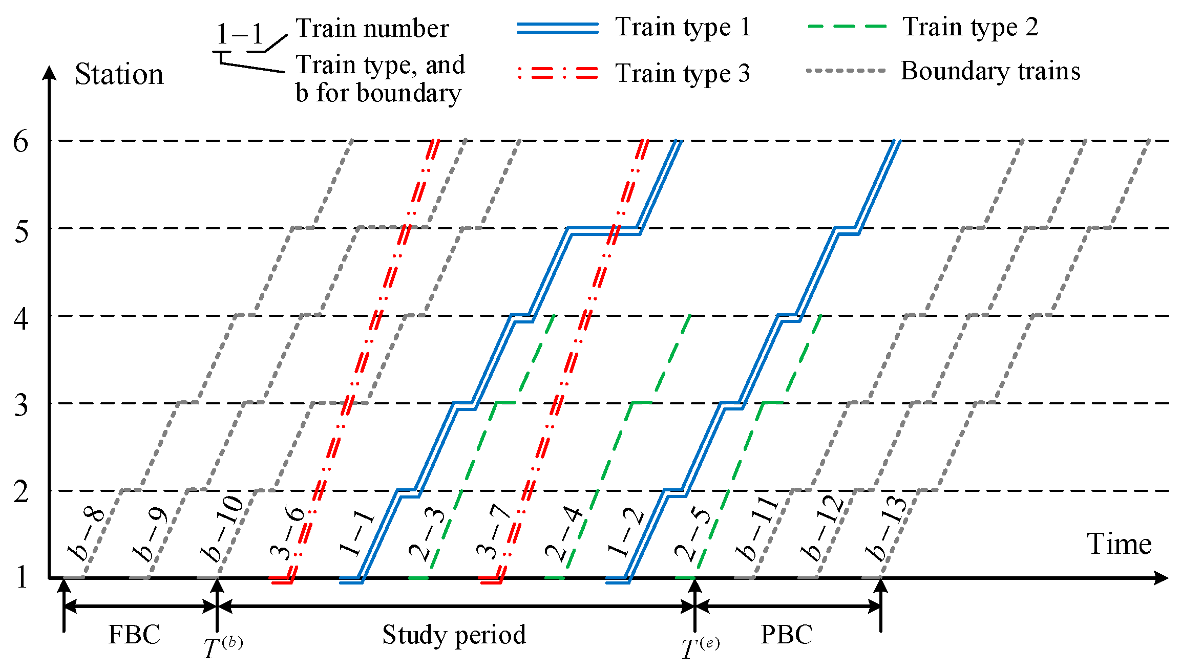
3.5. Boundary Conditions
3.6. Assumptions and Notations
4. Mathematical Formulation
4.1. Constraints
4.1.1. Train Arrival and Departure Times
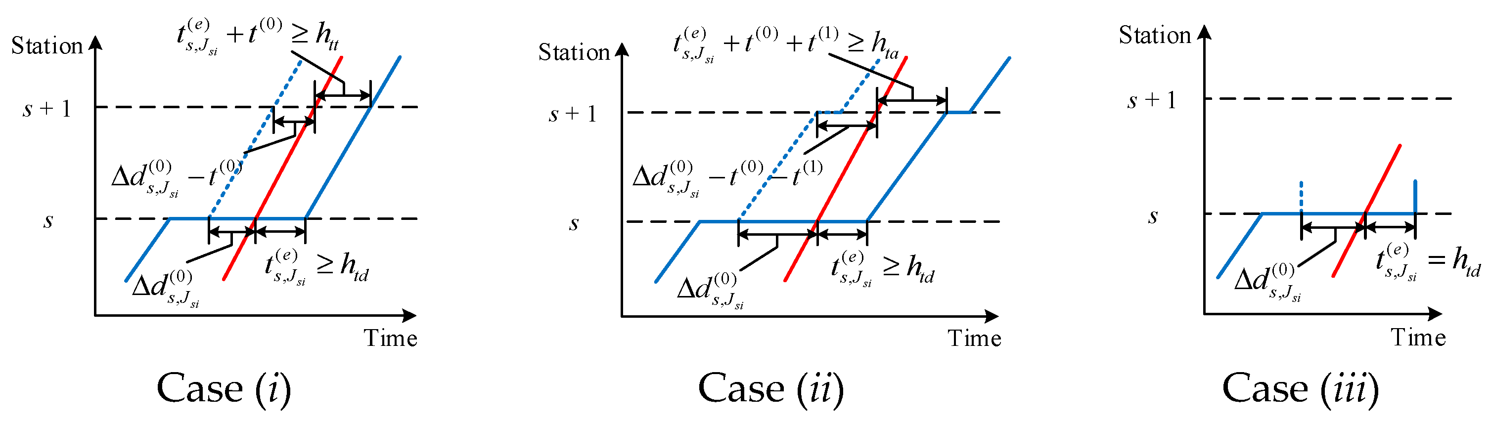
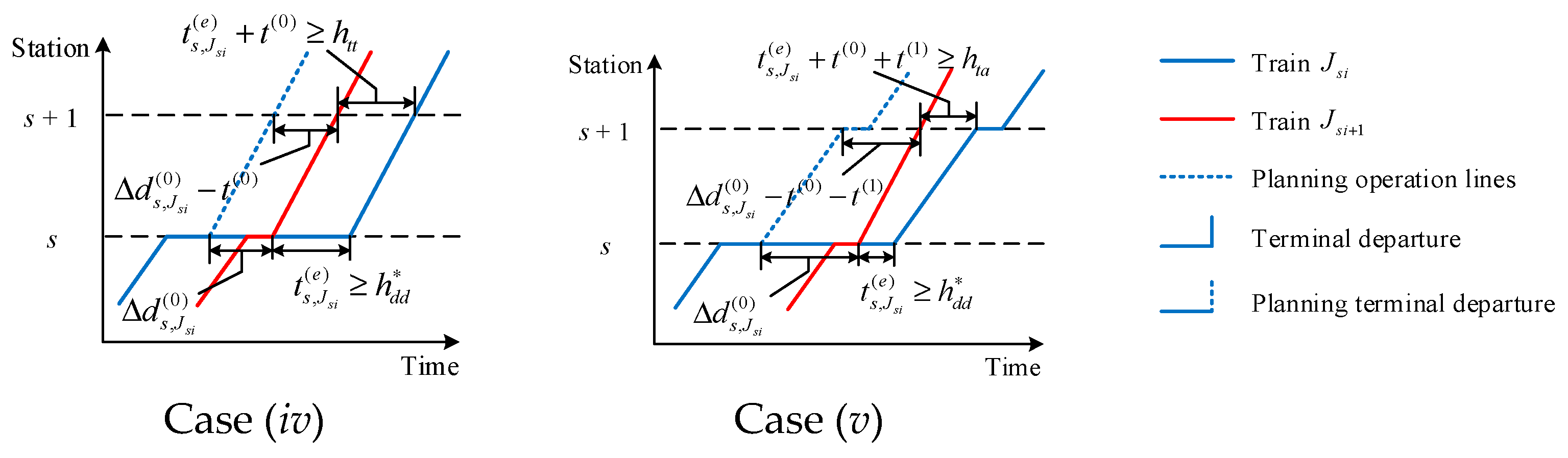
4.1.2. Operation Zone and Overtaking Station
- Case (i): train and train both operate at station s and s + 1, i.e., , and only train stops at station s, i.e., . Train will be overtaken by train with an extra dwell time when .
- Case (ii): train and train both operate at stations s and s + 1, and only train stops at stations s and s + 1, i.e., . Train will be overtaken by train with an extra dwell time when .
- Case (iii): train ends at station s and train operates at stations s and s + 1, i.e., , and train skips station s, i.e., . Train will be overtaken by train with an extra dwell time when .
- Case (iv): train and train both operate at stations s and s + 1, and both stop at only station s, i.e., . Train will be overtaken by train with an extra dwell time when .
- Case (v): train and train both operate at stations s and s + 1, and only train skips station s + 1, i.e., . Train will be overtaken by train with an extra dwell time when .
4.1.3. Train Capacity
4.1.4. Station Service
4.1.5. Vehicle Configuration
4.1.6. Other Constraints
4.2. Objective
4.2.1. System Life Cycle Cost
4.2.2. Total Passenger Travel Time Perception
4.3. Equilibrium Space–Time Network Design Model
5. Solution Algorithm
6. Case Study
6.1. Passenger Demand and Parameter Settings
6.2. Computational Result Analyses
6.3. Performance of the Number of Train Types
6.4. Performance of Different Strategies
6.5. Performance of Different Passenger Flow
7. Conclusions
Author Contributions
Funding
Institutional Review Board Statement
Informed Consent Statement
Data Availability Statement
Acknowledgments
Conflicts of Interest
Appendix A

| Parameters and Symbols | |
|---|---|
| The set of stations, , where S denotes the number of stations. | |
| The set of train types, , where the predefined constant K denotes the number of train types. | |
| The set of trains, where I denotes maximum number of trains during the optimization period . Let denotes the set of trains with the type trains. | |
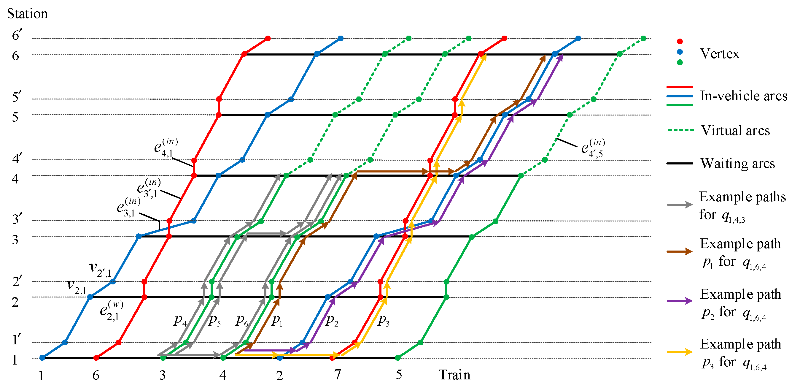
| The STN of timetable . The vertex set is , where and are the arrival and departure vertices of the train at the station , respectively. Each vertex contains time attributes that indicate the arrival or departure times of the train. The link set with time and capacity attributes contains the waiting arc and in-vehicle arc . Each link time contains the attributes of time and capacity referring to the train capacity or platform capacity at the station. | |
| The operation zone of type trains, where the superscript o indicates the origin stations and , and the superscript d indicates the destination stations and . | |
| Running segment of train , defined as . | |
| The length, running time, and passenger flow in running segment of train . | |
| Intervals. Symbols , and denote the minimum time interval between skipping–skipping, departure–skipping, skipping–departure, arrival–skipping, and skipping–arrival times of consecutive trains at each station, respectively; and denote the minimum interval between departures of consecutive trains at non-overtaking station and overtaking station, respectively; denotes turn-back operation time; and denotes maximum headway. | |
| Dwell times of train at station . Superscripts and indicate the minimum dwell time, actual dwell time, and additional dwell time due to overtaking, respectively. | |
| Running times of train at section . Superscripts and indicate the pure running time and the actual run time, respectively. | |
| The set of OD flows with timestamp. | |
| The index set of OD pairs with timestamp. | |
| Traction electricity, traction mechanical work, and resistance mechanical work of train . | |
| Traction inverter electrical efficiency, traction motor efficiency, and mechanical transmission efficiency from the output shaft of the traction motor to the wheels. | |
| Average mass of each motor vehicle, trailer vehicle, and passenger. | |
| The maximum loading rate of a train. | |
| Vehicle capacity with and without cab. | |
| Penalty values. Superscripts and indicate the penalty value of crowding and travel fatigue, respectively. | |
| Penalty threshold of crowding and travel fatigue. | |
| Auxiliary variables | |
| A binary variable, if the station is a turn-back station, 0 otherwise, i.e., if , otherwise . Superscript (0) indicates the real timetable. | |
| A binary variable, , if the station is an overtaking station, 0 otherwise, i.e., if otherwise . Superscript (0) indicates the real timetable. | |
| Number of vehicles belong to type train, number of total vehicles in our model and real timetable. | |
| Train order , which is an ordered I-tuple, at station in line plan , defined as a non-repeated arrangement of train number 1, 2, …, I, where is the I-dimensional Cartesian product of train set, and the element denotes the i-the arriving train is the train at station . | |
| The path–link incidence matrix in the space–time network. , where , if link belongs to path , 0 otherwise. | |
| The in-vehicle arc and link incidence matrix in the space–time network. , where , if in-vehicle arc is the link , 0 otherwise. | |
| The path–OD incidence matrix in the space–time network. , where , if path belongs to the OD pair , 0 otherwise. | |
| The train number and train type incidence matrix. , where , if train belongs to train type , 0 otherwise. | |
| Indicator vector of operation zones. , where , if , 0 otherwise. Note that the operation zones of the train can be calculated by . | |
| Arrival and departure time of train at station . Let with the superscript indicate the planning departure time. | |
| A binary variable. , if train overtakes train at station , 0 otherwise. | |
| Decision variable | |
| The line planning with the predefined set of train types. , where denotes the vector of stopping pattern, denotes the vector of train formation, and denotes the vector of train frequency for all type of trains. , if type trains stop at station , 0 otherwise. As for the stopping pattern of train , it can be calculated by Note that the operation zone for each train type can be calculated from the stopping pattern . | |
| The train arrival order at the first station under the line planning . Based on Assumption A.4, i.e., each type of train adheres to the principle of even-headway at their origin station within a short period, the departure times of trains from their origin station can be uniquely determined by the departure frequency . However, the departure times at other stations are influenced by the type of each train, i.e., the decision variables of the line plan, hence, the timetable will be uniquely determined by the arrival order of each type of train. | |
Appendix B
Appendix B.1. LCC of Infrastructure

Appendix B.2. LCC of Vehicle
Appendix B.3. Staff Cost
Appendix B.4. Other Costs
Appendix C
| Station | 1 | 2 | 3 | 4 | 5 | 6 | 7 | 8 | 9 | 10 | 11 | 12 | 13 | 14 |
| Dwell time/s | 45 | 30 | 30 | 30 | 35 | 30 | 30 | 30 | 30 | 30 | 30 | 35 | 45 | 35 |
| Section | 1–2 | 2–3 | 3–4 | 4–5 | 5–6 | 6–7 | 7–8 | 8–9 | 9–10 | 10–11 | 11–12 | 12–13 | 13–14 |
|---|---|---|---|---|---|---|---|---|---|---|---|---|---|
| Length/m | 2631 | 1275 | 2366 | 1982 | 993 | 1728 | 1090 | 1355 | 2337 | 2301 | 2055 | 1281 | 1334 |
| Running time/s | 190 | 108 | 157 | 135 | 90 | 114 | 103 | 104 | 164 | 150 | 140 | 102 | 105 |
| Parameters | Value | Parameters | Value | Parameters | Value |
|---|---|---|---|---|---|
| (s) | 6.03 × 10⁴ | (kg) | [3.5 × 10⁴, 3 × 10⁴] | (s) | {10, 9} |
| (CNY) | 3 × 10⁶ | (CNY) | 6.5 × 10⁶ | (s) | 120 |
| (CNY) | 1.4 × 10⁷ | (year) | 30 | (s) | 63 |
| (year) | 36 | 5% | (s) | 18 | |
| 4% | (CNY/kWh per vehicle) | 0.2289 | (s) | 45 | |
| (CNY/h) | 27.5839 | (CNY/kWh per vehicle) | 0.7047 | (s) | 150 |
| (CNY/h) | 24.9813 | (CNY/kWh per vehicle) | 1.1993 | (s) | 120 |
| 0.3021 | (CNY/h per vehicle) | 31.1813 | (s) | 45 | |
| 0.3298 | (CNY/kWh) | 0.7995 | (s) | 120 | |
| 0.7619 | (CNY/year) | 1.05×10⁴ | 0.18 | ||
| (passengers) | 230 | 150% | (s) | 540 | |
| (passengers) | 245 | (stations) | 5 | 0.6 | |
| (kg) | 65 | (s) | 900 | 0.45 |
| Parameters | Value | Parameters | Value | Parameters | Value |
|---|---|---|---|---|---|
| Population size in NSGA II | 96 | Population size in scheduling | 20 | Parameter in SAGP | 0.6 |
| Maximum iterations in NSGA II | 100 | Maximum iterations in scheduling | 50 | Tolerance error in SAGP | 10−1 |
| Crossover probability in NSGA II | 1 | Crossover probability in scheduling | 0.9 | in SAGP | 104 |
| Mutation probability in NSGA II | 0.1 | Mutation probability in scheduling | 0.1 | in SAGP | 100 |
| in NSGA II | 20 | Maximum iterations in SAGP | 30 | ||
| in NSGA II | 20 | Parameter in SAGP | 0.2 |
References
- Vuchic, V.R. Urban Transit: Operations, Planning, and Economics; John Wiley & Sons: Hoboken, NJ, USA, 2017. [Google Scholar]
- Sels, P.; Dewilde, T.; Cattrysse, D.; Vansteenwegen, P. Reducing the passenger travel time in practice by the automated construction of a robust railway timetable. Transp. Res. Part B Methodol. 2016, 84, 124–156. [Google Scholar] [CrossRef]
- Niu, H.; Zhang, M. An optimization to schedule train operations with phase-regular framework for intercity rail lines. Discret. Dyn. Nat. Soc. 2012, 2012, 549374. [Google Scholar] [CrossRef]
- Canca, D.; Barrena, E.; Laporte, G.; Ortega, F.A. A short-turning policy for the management of demand disruptions in rapid transit systems. Ann. Oper. Res. 2016, 246, 145–166. [Google Scholar] [CrossRef]
- Xu, X.; Li, C.; Xu, Z. Train timetabling with stop-skipping, passenger flow, and platform choice considerations. Transp. Res. Part B Methodol. 2021, 150, 52–74. [Google Scholar] [CrossRef]
- Mao, B.; Zheng, Z.; Chen, Z. A review on operational technologies of urban rail transit networks. J. Transp. Syst. Eng. Inf. Technol. 2017, 17, 155. [Google Scholar]
- Li, Z.; Mao, B.; Bai, Y.; Chen, Y. Integrated optimization of train stop planning and scheduling on metro lines with express/local mode. IEEE Access 2019, 7, 88534–88546. [Google Scholar] [CrossRef]
- Schöbel, A. An eigenmodel for iterative line planning, timetabling and vehicle scheduling in public transportation. Transp. Res. Part C Emerg. Technol. 2017, 74, 348–365. [Google Scholar] [CrossRef]
- Yang, L.; Qi, J.; Li, S.; Gao, Y. Collaborative optimization for train scheduling and train stop planning on high-speed railways. Omega-Int. J. Manage. Sci. 2016, 64, 57–76. [Google Scholar] [CrossRef]
- Sun, D.J.; Xu, Y.; Peng, Z.R. Timetable optimization for single bus line based on hybrid vehicle size model. J. Traffic Transp. Eng. (Engl. Ed.) 2015, 2, 179–186. [Google Scholar] [CrossRef]
- Nuzzolo, A.; Crisalli, U.; Rosati, L. A schedule-based assignment model with explicit capacity constraints for congested transit networks. Transp. Res. Part C Emerg. Technol. 2012, 20, 16–33. [Google Scholar] [CrossRef]
- An, J.; Uno, N.; Yang, X.; Liu, H.; Shiomi, Y. Measurement of travel fatigue: Objective monitoring and subjective estimation. Transp. Res. Rec. 2011, 2216, 157–164. [Google Scholar] [CrossRef]
- Qi, J.; Li, S.; Gao, Y.; Yang, K.; Liu, P. Joint optimization model for train scheduling and train stop planning with passengers distribution on railway corridors. J. Oper. Res. Soc. 2018, 69, 556–570. [Google Scholar] [CrossRef]
- de Palma, A.; Lindsey, R. Optimal timetables for public transportation. Transp. Res. Part B Methodol. 2001, 35, 789–813. [Google Scholar] [CrossRef]
- Hansen, I.; Pachl, J. Railway Timetabling and Operations: Analysis, Modelling, Optimisation, Simulation, Performance, Evaluation; Eurail Press: Utrecht, The Netherlands, 2014. [Google Scholar]
- Yang, X.; Li, X.; Gao, Z.; Wang, H.; Tang, T. A cooperative scheduling model for timetable optimization in subway systems. IEEE Trans. Intell. Transp. Syst. 2012, 14, 438–447. [Google Scholar] [CrossRef]
- Yuan, J.; Gao, Y.; Li, S.; Liu, P.; Yang, L. Integrated optimization of train timetable, rolling stock assignment and short-turning strategy for a metro line. Eur. J. Oper. Res. 2022, 301, 855–874. [Google Scholar] [CrossRef]
- Lee, Y.J.; Shariat, S.; Choi, K. Mathematical modeling for optimizing skip-stop rail transit operation strategy using genetic algorithm. In Proceedings of the Transportation Research Board Meeting, Stockholm, Sweden, 4–6 September 2013. [Google Scholar]
- Cadarso, L.; Marín, Á. Robust rolling stock in rapid transit networks. Comput. Oper. Res. 2011, 38, 1131–1142. [Google Scholar] [CrossRef]
- Hao, L.; Qin, J.; Yang, X.S.; Zhou, W.; Xie, C. Joint train line planning and timetabling of intercity high-speed rail with actual time-dependent demand. Int. J. Transp. Sci. Technol. 2023, 12, 534–548. [Google Scholar] [CrossRef]
- Zhang, C.; Qi, J.; Gao, Y.; Yang, L.; Gao, Z.; Meng, F. Integrated optimization of line planning and train timetabling in railway corridors with passengers’ expected departure time interval. Comput. Ind. Eng. 2021, 162, 107680. [Google Scholar] [CrossRef]
- Mei, W.; Zhang, Y.; Zhang, M.; Qing, G.; Zhang, Z. Research on line planning and timetabling optimization model based on passenger flow of subway network. Vehicles 2022, 4, 375–389. [Google Scholar] [CrossRef]
- Cortés, C.E.; Jara-Díaz, S.; Tirachini, A. Integrating short turning and deadheading in the optimization of transit services. Transp. Res. Part A Policy Pract. 2011, 45, 419–434. [Google Scholar] [CrossRef]
- Tirachini, A.; Cortés, C.E.; Jara-Díaz, S.R. Optimal design and benefits of a short turning strategy for a bus corridor. Transportation 2011, 38, 169–189. [Google Scholar] [CrossRef]
- Chang, Y.; Yeh, C.; Shen, C. A multiobjective model for passenger train services planning: Application to Taiwan’s high-speed rail line. Transp. Res. Part B Methodol. 2000, 34, 91–106. [Google Scholar] [CrossRef]
- Nesheli, M.M.; Ceder, A.A.; Liu, T. A robust, tactic-based, real-time framework for public-transport transfer synchronization. Transp. Res. Procedia 2015, 9, 246–268. [Google Scholar] [CrossRef]
- Lu, C.; Tang, J.; Zhou, L.; Yue, Y.; Huang, Z. Improving recovery-to-optimality robustness through efficiency-balanced design of timetable structure. Transp. Res. Part C Emerg. Technol. 2017, 85, 184–210. [Google Scholar] [CrossRef]
- Zhang, Y.; Peng, Q.; Lu, G.; Zhong, Q.; Yan, X.; Zhou, X. Integrated line planning and train timetabling through price-based cross-resolution feedback mechanism. Transp. Res. Part B Methodol. 2022, 155, 240–277. [Google Scholar] [CrossRef]
- Zhou, W.; Oldache, M. Integrated optimization of line planning, timetabling and rolling stock allocation for urban railway lines. Sustainability 2021, 13, 13059. [Google Scholar] [CrossRef]
- Yang, R.; Han, B.; Zhang, Q.; Han, Z.; Long, Y. Integrated optimization of train route plan and timetable with dynamic demand for the urban rail transit line. Transp. B Transp. Dyn. 2023, 11, 93–126. [Google Scholar] [CrossRef]
- Li, C.; Tang, J.; Zhang, J.; Zhao, Q.; Wang, L.; Li, J. Integrated optimization of urban rail transit line planning, timetabling and rolling stock scheduling. PLoS ONE 2023, 18, e0285932. [Google Scholar] [CrossRef] [PubMed]
- Chen, Q. Global optimization for bus line timetable setting problem. Discret. Dyn. Nat. Soc. 2014, 2014, 636937. [Google Scholar] [CrossRef]
- Zhu, Y.; Mao, B.; Bai, Y.; Chen, S. A bi-level model for single-line rail timetable design with consideration of demand and capacity. Transp. Res. Part C Emerg. Technol. 2017, 85, 211–233. [Google Scholar] [CrossRef]
- Zhang, T.; Li, D.; Qiao, Y. Comprehensive optimization of urban rail transit timetable by minimizing total travel times under time-dependent passenger demand and congested conditions. Appl. Math. Model. 2018, 58, 421–446. [Google Scholar] [CrossRef]
- Zhang, M.; Wang, Y.; Su, S.; Tang, T.; Ning, B. A short turning strategy for train scheduling optimization in an urban rail transit line: The case of Beijing subway line 4. J. Adv. Transp. 2018, 2018, 5367295. [Google Scholar] [CrossRef]
- Dong, X.; Li, D.; Yin, Y.; Ding, S.; Cao, Z. Integrated optimization of train stop planning and timetabling for commuter railways with an extended adaptive large neighborhood search metaheuristic approach. Transp. Res. Part C Emerg. Technol. 2020, 117, 102681. [Google Scholar] [CrossRef]
- Yue, Y.; Wang, S.; Zhou, L.; Tong, L.; Saat, M.R. Optimizing train stopping patterns and schedules for high-speed passenger rail corridors. Transp. Res. Part C Emerg. Technol. 2016, 63, 126–146. [Google Scholar] [CrossRef]
- Jiang, F.; Cacchiani, V.; Toth, P. Train timetabling by skip-stop planning in highly congested lines. Transp. Res. Part B Methodol. 2017, 104, 149–174. [Google Scholar] [CrossRef]
- Zhu, Y.; Goverde, R.M.P. Railway timetable rescheduling with flexible stopping and flexible short-turning during disruptions. Transp. Res. Part B Methodol. 2019, 123, 149–181. [Google Scholar] [CrossRef]
- Li, Y.; Han, B.; Yang, R.; Zhao, P. Integrated optimization of stop planning and timetabling for demand-responsive transport in high-speed railways. Appl. Sci. 2022, 13, 551. [Google Scholar] [CrossRef]
- Wang, Y.; De Schutter, B.; van den Boom, T.J.; Ning, B.; Tang, T. Efficient bilevel approach for urban rail transit operation with stop-skipping. IEEE Trans. Intell. Transp. Syst. 2014, 15, 2658–2670. [Google Scholar] [CrossRef]
- Zhao, Y.; Li, D.; Yin, Y.; Zhao, X. Integrated optimization of demand-driven timetable, train formation plan and rolling stock circulation with variable running times and dwell times. Transp. Res. Part E Logist. Transp. Rev. 2023, 171, 103035. [Google Scholar] [CrossRef]
- Karp, R.M. On the computational complexity of combinatorial problems. Networks 1975, 5, 45–68. [Google Scholar] [CrossRef]
- Mejía-De-Dios, J.A.; Rodríguez-Molina, A.; Mezura-Montes, E. Multiobjective bilevel optimization: A survey of the state-of-the-art. IEEE Trans. Syst. Man Cybern. Syst. 2023, 53, 5478–5490. [Google Scholar] [CrossRef]
- Deb, K.; Pratap, A.; Agarwal, S.; Meyarivan, T. A fast and elitist multiobjective genetic algorithm: NSGA-II. IEEE Trans. Evol. Comput. 2002, 6, 182–197. [Google Scholar] [CrossRef]
- Levitin, E.S.; Polyak, B.T. Constrained minimization methods. USSR Comput. Math. Math. Phys. 1966, 6, 1–50. [Google Scholar] [CrossRef]
- Goldstein, A.A. Convex Programming in Hilbert Space. Bull. Am. Math. Soc. 1964, 70, 709–710. [Google Scholar] [CrossRef]
- He, B.S.; Yang, H.; Meng, Q.; Han, D.R. Modified Goldstein–Levitin–Polyak projection method for asymmetric strongly monotone variational inequalities. J. Optim. Theory Appl. 2002, 112, 129–143. [Google Scholar] [CrossRef]
- Han, D.; Sun, W. A new modified Goldstein-Levitin-Polyak projection method for variational inequality problems. Comput. Math. Appl. 2004, 47, 1817–1825. [Google Scholar] [CrossRef]
- Chen, A.; Zhou, Z.; Xu, X. A self-adaptive gradient projection algorithm for the nonadditive traffic equilibrium problem. Comput. Oper. Res. 2012, 39, 127–138. [Google Scholar] [CrossRef]
- Tang, L.; D Ariano, A.; Xu, X.; Li, Y.; Ding, X.; Samà, M. Scheduling local and express trains in suburban rail transit lines: Mixed–integer nonlinear programming and adaptive genetic algorithm. Comput. Oper. Res. 2021, 135, 105436. [Google Scholar] [CrossRef]
- Gao, Y.; Yang, L.; Gao, Z. Energy consumption and travel time analysis for metro lines with express/local mode. Transp. Res. Part D Transp. Environ. 2018, 60, 7–27. [Google Scholar] [CrossRef]
- Hamdouch, Y.; Marcotte, P.; Nguyen, S. A strategic model for dynamic traffic assignment. Netw. Spat. Econ. 2004, 4, 291–315. [Google Scholar] [CrossRef]
- Nagurney, A. Network Economics: A Variational Inequality Approach; Springer Science & Business Media: Berlin/Heidelberg, Germany, 1998. [Google Scholar]
- Gabriel, S.A.; Bernstein, D. The traffic equilibrium problem with nonadditive path costs. Transp. Sci. 1997, 31, 337–348. [Google Scholar] [CrossRef]
- Smith, M.J. The existence, uniqueness and stability of traffic equilibria. Transp. Res. Part B Methodol. 1979, 13, 295–304. [Google Scholar] [CrossRef]


| Indicators | Time-Varying Frequency | Multiple Turn-Backs | Express/Local Stopping | Variable Train Lengths |
|---|---|---|---|---|
| Temporal imbalance of train load | − | − | ||
| Spatial imbalance of train load | − | − | ||
| Imbalance of station load | − | − | ||
| Operator cost | ± | − | ± | − |
| Total waiting time | − | ± | + | |
| Total passenger In-vehicle time | − | |||
| Total passenger Transfer time | + | + | − |
Disclaimer/Publisher’s Note: The statements, opinions and data contained in all publications are solely those of the individual author(s) and contributor(s) and not of MDPI and/or the editor(s). MDPI and/or the editor(s) disclaim responsibility for any injury to people or property resulting from any ideas, methods, instructions or products referred to in the content. |
© 2024 by the authors. Licensee MDPI, Basel, Switzerland. This article is an open access article distributed under the terms and conditions of the Creative Commons Attribution (CC BY) license (https://creativecommons.org/licenses/by/4.0/).
Share and Cite
Gao, Y.; Jia, C.; Wang, Z.; Hu, Z. A Cost-Effective Approach for the Integrated Optimization of Line Planning and Timetabling in an Urban Rail Transit Line. Appl. Sci. 2024, 14, 6273. https://doi.org/10.3390/app14146273
Gao Y, Jia C, Wang Z, Hu Z. A Cost-Effective Approach for the Integrated Optimization of Line Planning and Timetabling in an Urban Rail Transit Line. Applied Sciences. 2024; 14(14):6273. https://doi.org/10.3390/app14146273
Chicago/Turabian StyleGao, Yi, Chuanjun Jia, Zhipeng Wang, and Zhiyuan Hu. 2024. "A Cost-Effective Approach for the Integrated Optimization of Line Planning and Timetabling in an Urban Rail Transit Line" Applied Sciences 14, no. 14: 6273. https://doi.org/10.3390/app14146273
APA StyleGao, Y., Jia, C., Wang, Z., & Hu, Z. (2024). A Cost-Effective Approach for the Integrated Optimization of Line Planning and Timetabling in an Urban Rail Transit Line. Applied Sciences, 14(14), 6273. https://doi.org/10.3390/app14146273