Stress–Dilatancy Behavior of Alluvial Sands

Abstract

Based on the Frictional State Concept (FSC), the stress–dilatancy behavior of alluvial sands in drained triaxial compression was investigated. The dilatant failure state is equivalent to the minimum plastic dilatancy state for sands. The dilatant failure state slightly precedes the failure state. The straight line approximating dilatant failure states in the stress ratio–plastic dilatancy plane defines the slope of the critical frictional state line in the q-p’ plane, i.e., the critical frictional state angle. The stress ratio–plastic dilatancy relationship, obtained from the FSC, defines the sand shear angle as a function of the critical frictional state angle and plastic dilatancy. The shear angle of the tested sand is a maximum of 2° greater than that obtained from Bolton’s formula. According to the authors, these differences are affected by the transverse anisotropy of sand in the tested samples and the difference between the dilatant failure state and the failure state.

1. Introduction

A characteristic feature of soils and other geomaterials is the change in volume caused by shear deformations. This phenomenon is called dilatancy. Stress–dilatancy, or more precisely, stress ratio–plastic dilatancy, plays a crucial role in the elastoplastic modeling of geomaterials [1,2,3].

The best-known is Bolton’s stress–dilatancy relationship for sand, which takes the critical state as the reference state. The critical state for sand is reached at large shear strains [4]. In the critical state, non-uniform stresses and strains are observed in the tested sample due to the formation of a shear band in dense sand samples and the barreling of loose sand samples [5,6,7,8]. The non-uniform sample deformation during shearing is a fundamental difficulty in correctly identifying the soil strength and stress–strain relationship [6]. The shear strength of sand, dilatancy, and critical state angle depend on the size and shape of sand particles [9]. The anisotropy of the sand in the tested sample may result from the method of sample preparation in the laboratory [7,9]. Transverse anisotropy is observed in gravity-deposited soils. Therefore, a sand sample taken in situ or formed by the dry pluviation method has transverse anisotropy [10].

The Frictional State Concept (FSC) was formulated by Szypcio [11]. The general stress ratio–plastic dilatancy relationship obtained from the FSC is defined by the critical frictional state angle (${\varphi }^o$) and two parameters of the FSC ($\alpha$ and $\beta$). These two parameters represent the deviation in the dissipated energy in the current state from the energy dissipated in the critical frictional state (CFS) as the reference state. The CFS can be treated as an extension of the critical state. The critical state angle and critical frictional state angle are equal for sands (${\varphi }^o={\varphi }_{cs}$).

In this work, the conventional drained triaxial compression test results of alluvial sand were analyzed in light of the FSC. It is shown that the dilatant failure states and the failure state are slightly different.

2. Stress Ratio–Plastic Dilatancy Relationship

The general stress ratio–plastic dilatancy relationship obtained using the FSC [11] is

$$\eta =Q-A{D}^p,$$

(1)

where

$$Q=M^o-\alpha A^o,$$

(2)

$$A=\beta A^o,$$

(3)

$$A^o=1-M^o\left(\delta q/\delta p^{\prime }\right),$$

(4)

$$D^p=\delta {\epsilon }_{\upsilon }^p/\delta {\epsilon }_q^p.$$

(5)

$\alpha$ and $\beta$ are FSC parameters, and $D^p$ is the plastic dilatancy. For drained triaxial compression with ${\sigma }_3^{\prime }=$ constant, $\delta q/\delta p^{\prime }=3$ [11] and

$$M^o=M_c^o=6 sin{\varphi }^o/\left(3-sin{\varphi }^o\right),$$

(6)

$$A^o=A_c^o=1-{\displaystyle \frac{1}{3}}{M}_c^o,$$

(7)

$$q={\sigma }_1^{\prime }-{\sigma }_3^{\prime }={\sigma }_a^{\prime }-{\sigma }_r^{\prime },$$

(8)

$$p^{\prime }={\displaystyle \frac{1}{3}}\left({\sigma }_1^{\prime }+2{\sigma }_3^{\prime }\right)={\displaystyle \frac{1}{3}}\left({\sigma }_a^{\prime }+2{\sigma }_r^{\prime }\right),$$

(9)

$$\delta {\epsilon }_{\upsilon }={\delta \epsilon }_1+2{\delta \epsilon }_3={\delta \epsilon }_a+2{\delta \epsilon }_r,$$

(10)

$$\delta {\epsilon }_q={\displaystyle \frac{2}{3}}\left({\delta \epsilon }_1+{\delta \epsilon }_3\right)={\displaystyle \frac{2}{3}}\left({\delta \epsilon }_a+2{\delta \epsilon }_r\right),$$

(11)

$$\delta {\epsilon }_{\upsilon }^p={\delta \epsilon }_{\upsilon }-{\delta \epsilon }_{\upsilon }^e,$$

(12)

$$\delta {\epsilon }_q^p={\delta \epsilon }_q-{\delta \epsilon }_q^e,$$

(13)

where

$$\delta {\epsilon }_{\upsilon }^e=\delta p^{\prime }/K,$$

(14)

$$\delta {\epsilon }_q^e=\delta q/3G.$$

(15)

$K$ and $G$ are the elastic bulk and shear moduli. The line representing the purely frictional state is called the frictional state line (FSL) and is defined by Equation (1) with $\alpha =$ 0 and $\beta =$ 1.0 [11]. The dilatant failure state (DFS) is defined as the state with the minimum value of the plastic dilatancy ($D_{min}^p$) state [11]. The line representing the DFS is called the dilatant failure state line (DFSL) equivalent to the FSL and is defined by Equation (1) with $\alpha ={\alpha }_f=0$ and $\beta ={\beta }_f=1$ for sands without breakage effects [11]. The stress ratio–plastic dilatancy relationship (1) is a form of the energy balance equation [11]. The FSL for sand sheared under conventional drained triaxial compression with low and medium stress levels, without breakage effects, represents the fully frictional states ($\alpha$ = 0, $\beta$ = 1). The stress ratio ($\eta$) is dependent, but the energy dissipated during shear is not dependent on plastic dilatancy for these states [11]. The FSL is defined only by the critical friction state angle (${\varphi }^o$) for conventional drained triaxial compression. This is a very important conclusion from the FSC.

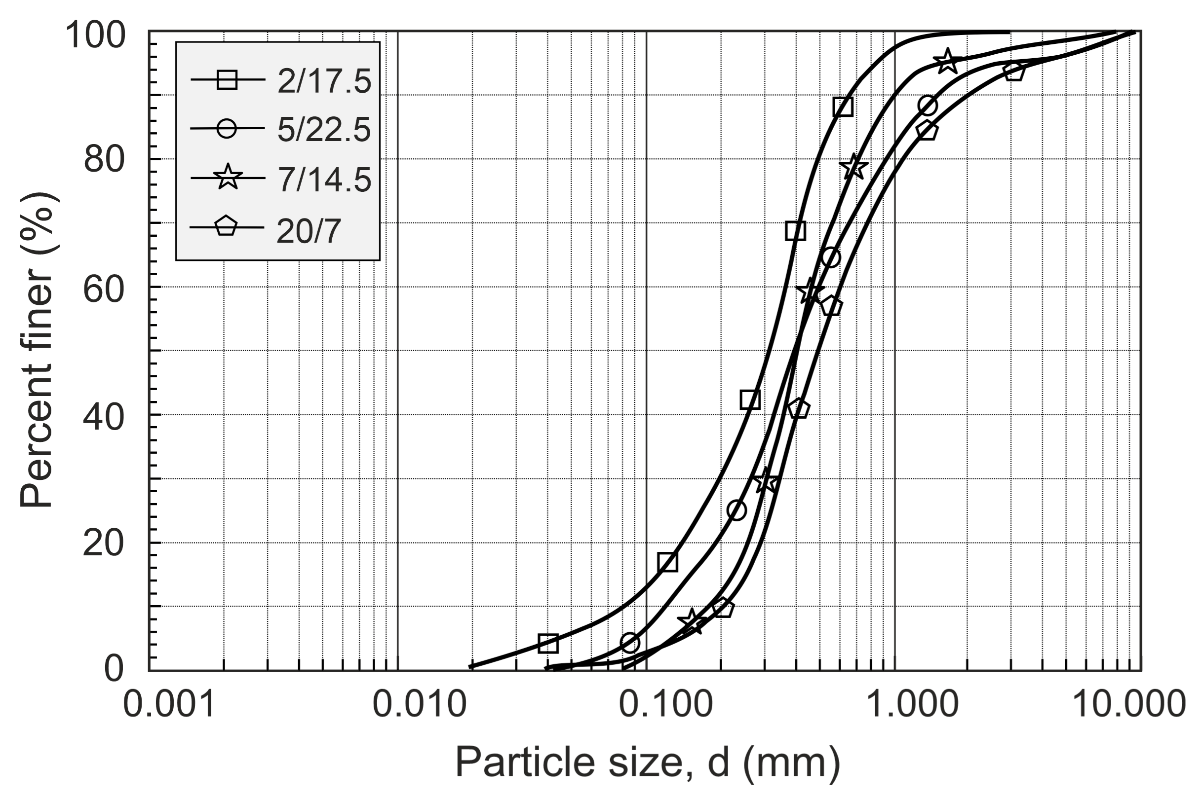
3. Material and Tests

The samples utilized in this study were obtained as part of a broader investigation, during which approximately 20 samples were collected for analysis. The majority of the samples were cohesive soil samples, and only non-cohesive soil samples were selected for testing in this study. The samples were collected using Class 1 samplers. The names of the sand samples shown in

Table 1. Physical characteristics of sand samples.

Sample	D50 mm	Cu -	Cc -	Gs -	emax -	emin -	Dr %
TXCD 2/17.5	0.32	5.03	1.39	2.66	0.75	0.36	0.93
TXCD 5/22.5	0.50	3.39	0.94	2.66	0.70	0.38	0.95
TXCD 7/14.5	0.43	4.05	1.13	2.66	0.73	0.41	0.82
TXCD 20/7	0.42	2.76	1.18	2.66	0.71	0.40	0.60

(the number before the slash) refer to the order in which all samples were taken, and the value after the slash refers to the sampling depth. The in situ density value of the samples was determined by field tests (CPT) and then used to reproduce this state in the laboratory.

The samples were taken from the lower section of the Oder River valley; therefore, the soil can be described as alluvial soil–river sand. Particle size distribution curves for the sands are shown in Figure 1, and the physical characteristics of the sands are summarized in Table 1. The coefficient of uniformity (C_u) ranges from 2.76 to 5.03, the coefficient of curvature (C_c) ranges from 0.94 to 1.39, and the median particle size (D₅₀) ranges from 0.32 to 0.50 mm. The sands also differ in terms of the maximum void ratio (0.70 to 0.75) and minimum void ratio (0.36 to 0.40). All sands are characterized by the same specific gravity value (2.66).

The triaxial compression tests were conducted using the drainage method. The tests were performed on dry pluviated samples, which were compacted to a relative density of the soil corresponding to the degree of compaction determined by the in situ tests. This method was chosen because it is commonly used in geotechnical engineering to produce uniform sand samples for laboratory testing. The method involves allowing dry sand to pluviate through the air into a container, producing a sample with a controlled density and structure. Dry pluviation is favored for its simplicity and ability to produce samples with uniform density and structure, making it ideal for various geotechnical tests such as triaxial compression tests, direct shear tests, and permeability tests. The relative density was different for each sample, as shown in Table 1. The soils tested can be classified as medium and very dense [12]. The samples were saturated using the back-pressure method until the value of the Skempton parameter was greater than or equal to 0.95 or until the maximum value was obtained [13]. The specimens were then isotropically consolidated to a pre-selected effective stress value. The measurement of changes in the volume of samples during the test was carried out using state-of-the-art pressure and volume controllers from GDS Instruments. The volumetric strain was determined by measuring the volume of water flowing out of the soil sample and was carried out using a volume controller.

The controller has a volume of 200 mL with a resolution of 1 mm³ and can maintain pressure up to a value of 2 MPa. Volume measurements were carried out with an accuracy of 0.05% over the full measurement range. The axial load was measured using an internal submersible load cell with a range of 10 kN and a resolution of 0.001 kN. The specimen’s axial strain was measured using a displacement sensor located outside the triaxial chamber, with a resolution of 0.001 mm. Cell and pore pressure was measured using external pressure transducers. Data were recorded for each second. After the consolidation was completed, the determination of shear and compressional wave velocities was carried out using Bender-type elements. The study employed piezoelectric transducers constructed by using EKULIT UPF-76Q-220 piezoelectric elements (EKULIT Elektrotechnik, Karl-Heinz Mauz GmbH Felix-Wankel-Str. 35 73760 Ostfildern, Germany), which exhibited a maximum operating voltage of 250 V and an electrical capacitance of 9 nF. These elements were cut to a dimension of 12 × 10 mm. To provide protection against mechanical damage and surges, shielded signal wires embedded in epoxy resin were attached to the prepared elements. An arbitrary GW-Instek AFG 2012 (GW-Instek, Taiwan, Taipei) signal generator was used to generate any waveform at a preset frequency, while a PicoScope 3203D digital 12-bit oscilloscope (Pico Technology, James House Colmworth Business Park St Neots Cambridgeshire PE19 8YP, UK) was used to receive the signals. During the course of the test, a sinusoidal signal with a frequency of 10 kHz and an amplitude of 20 V was applied to the samples. In the analysis of the signal, a method of visual interpretation of the signal was applied, where the main signal “peak” transition measurement focused on the major first peak method. On this basis, the values of the maximal shear (G) and bulk (K) moduli and the values of Poisson’s ratio were determined according to the following formulae:

$$G={\rho V}_s^2,$$

(16)

$$K=\rho \left(V_P^2-{\displaystyle \frac{4}{3}}{V}_S^2\right),$$

(17)

$$\nu ={\displaystyle \frac{V_p^2-2\times V_s^2}{\left(V_p^2-V_s^2\right)\times 0.5}}.$$

(18)

where:

• $\rho$—the bulk density [Mg/m³];
• $\nu$—Poisson’s ratio [-];
• $V_s$—the velocity of the propagation of the shear wave in the ground medium [m/s];
• $V_p$—the velocity of the propagation of the compression wave in the ground medium [m/s].

The shear (G) and bulk (K) moduli are expressed in MPa.

Specimens were sheared until the axial strain reached 15%. Shearing was conducted at a speed of 0.15 mm/minute.

4. Methodology

To calculate the stress ratio–plastic dilatancy relationship for the tested soil, it is convenient to express the values $q$, $p^{\prime }$, and ${\epsilon }_{\upsilon }$ as analytical functions of ${\epsilon }_a$ (${\epsilon }_q$). The analyzed values of the stresses and strains were unstable at the onset of shearing. Similar unstable behavior was observed during triaxial compression of medium-density chalk [14]. Therefore, these unstable values were eliminated in the first step. For example, the methodology for defining this instability region is shown in Figure 2 for the TXC 7/14.5 test at ${\sigma }_3^{\prime }={\sigma }_r^{\prime }=150 \mathrm{k}\mathrm{P}\mathrm{a}$.

The ${\Delta \epsilon }_a$ values for all analyzed tests are shown in

Table 2. The ${\Delta \epsilon }_a$ values for the analyzed tests.

Test	TXCD 2/17.5		TXCD 5/22.5			TXCD 7/14.5			TXCD 20/7
${\sigma }_3^{\prime }$ (kPa)	170	370	220	420	720	75	150	350	70	470
${\Delta \epsilon }_a$ (%)	0.095	0.384	0.209	0.003	0.222	0.002	0.808	0.529	0.001	0.007

.

In the second step, the corrected values of the axial strains ${\overline{\epsilon }}_a={\epsilon }_a-{\Delta \epsilon }_a$ were taken into account for analysis for ${\overline{\epsilon }}_a=0,$ $q=0$, $p^{\prime }=p_0={\sigma }_3^{\prime }={\sigma }_r^{\prime }$, and ${\epsilon }_{\upsilon }=0$. The experimental relationships $q-{\overline{\epsilon }}_a$, $p^{\prime }-{\overline{\epsilon }}_a$, and ${\epsilon }_{\upsilon }-{\overline{\epsilon }}_a$ were approximated by segments using high-degree polynomials (Figure 2).

Attention was paid to the continuity of not only the values of the approximated quantities but also the increment ratios ($\delta q/\delta {\overline{\epsilon }}_a$, $\delta p^{\prime }/\delta {\overline{\epsilon }}_a$, $\delta {\epsilon }_{\upsilon }/\delta {\overline{\epsilon }}_a$) at the segment connection points (Figure 2). The continuity of $\delta {\epsilon }_{\upsilon }/\delta {\overline{\epsilon }}_a$ is particularly important for further analysis.

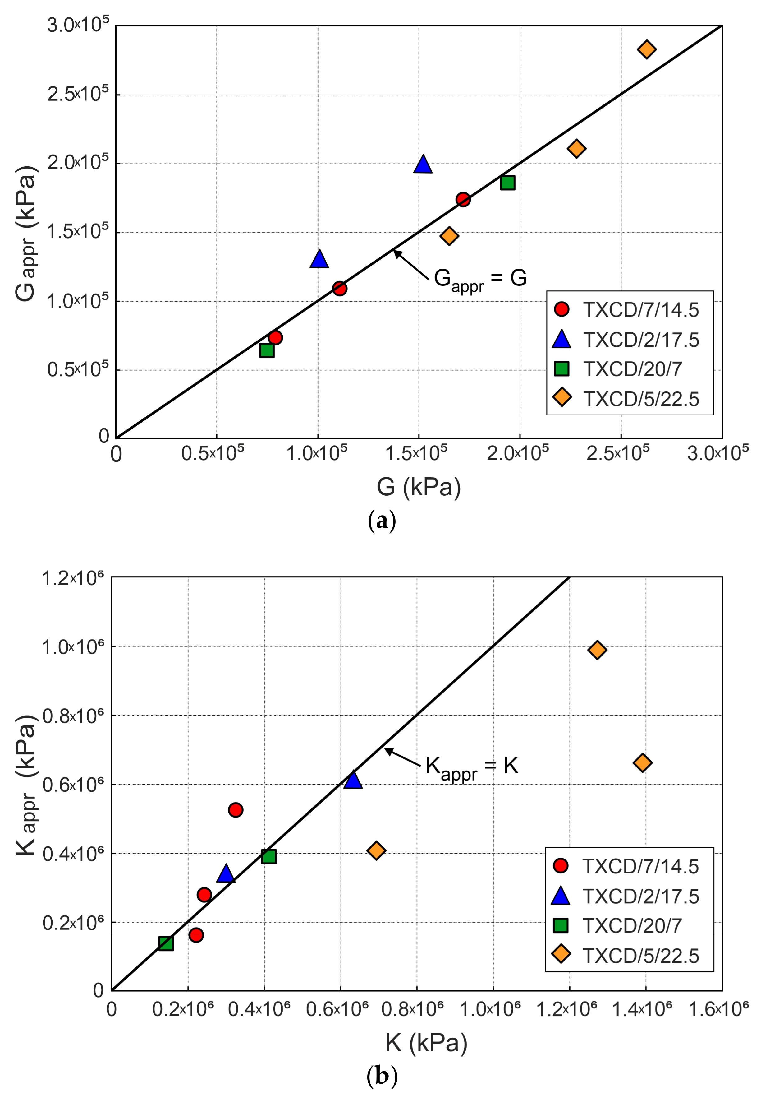
5. Elasticity Parameters

Assuming the elastic behavior of sand at the onset of shear, the elastic parameters can be calculated using the formulae

$$G^{*}=\delta q/3\delta {\epsilon }_q,$$

(19)

$$K^{*}=\delta p^{\prime }/\delta {\epsilon }_{\upsilon },$$

(20)

$${\nu }^{*}={\displaystyle \frac{3K^{*}-2G^{*}}{2\left(3K^{*}+G^{*}\right)}}.$$

(21)

A superscript index (*) has been introduced to distinguish elastic parameters for small strains (${\overline{\epsilon }}_a=$ 0.1%), calculated from Equations (16)–(18), from elastic parameters for very small strains obtained by analyzing the propagation of the shear and compression wave velocities in the sample (

Table 3. Elastic parameters for tested sands.

Test	TXCD 2/17.5		TXCD 5/22.5			TXCD 7/14.5			TXCD 20/7
${\sigma }_3^{\prime }$ (kPa)	170	370	220	420	720	75	150	350	70	470
$G$ (MPa)	101.0	152.0	165.0	228.0	263.0	79.0	111.0	172.0	75.0	194.0
$K$ (MPa)	300.0	633.3	695.0	1393.0	1274.2	218.9	243.0	325.8	147.0	384.9
$\nu$ (-)	0.36	0.40	0.39	0.32	0.28	0.35	0.31	0.28	0.28	0.29
$G^{*}$ (MPa)	25.6	29.5	146.3	102.6	160.8	10.0	28.3	32.7	45.4	25.8
$K^{*}$ (MPa)	43.2	53.5	247.2	132.4	166.0	24.7	39.2	64.3	95.8	38.0
${\nu }^{*}$ (-)	0.25	0.27	0.25	0.19	0.13	0.32	0.21	0.28	0.30	0.22
${\alpha }_G$ (-)	3.94	5.25	1.13	2.22	1.64	7.90	3.92	5.26	1.65	7.52
${\alpha }_K$ (-)	6.54	11.84	2.81	10.5	7.67	8.86	6.20	5.07	1.53	10.13

). The values $G^{*}$ and $K^{*}$ are usually smaller than $G$ and $K$ [15].

The differences can be expressed by

$${\alpha }_G=G/G^{*},$$

(22)

$${\alpha }_K=K/K^{*}.$$

(23)

The elastic parameters for small and very small strains are presented in Table 3.

Usually, it is assumed that the elastic parameters of sand depend on the void ratio ($e$) and effective mean stress ($p^{\prime }$) [16]. In this paper, it is assumed that the elasticity parameters at very small strains can be approximated by the following formulae:

$$G_{appr}=A_G p_a {\displaystyle \frac{{\left(e_G-e\right)}^2}{1+e}}{\left({\displaystyle \frac{p^{\prime }}{p_a}}\right)}^{a_G},$$

(24)

$$K_{appr}=A_K p_a {\displaystyle \frac{{\left(e_K-e\right)}^2}{1+e}}{\left({\displaystyle \frac{p^{\prime }}{p_a}}\right)}^{a_K},$$

(25)

$${\nu }_{appr}={\displaystyle \frac{3K_{appr}-2G_{appr}}{2\left(3K_{appr}+G_{appr}\right)}},$$

(26)

where $A_G=220$, $A_K=520$, $e_G=e_K=2.87$, $a_G=0.55$, $a_K=0.75,$ and the atmospheric pressure $p_a=101$ kPa. The parameters $e_G$ and $a_G$ are very similar to those given by Hardin and Richart [16] ($e_G=2.97$ and $a_G=0.5$). $G$, $K$, $G_{appr}$, and $K_{appr}$ are shown in Figure 3.

The parameters $G=G_{appr}$ and ${K=K}_{appr}$ were used for further analysis (Figure 3).

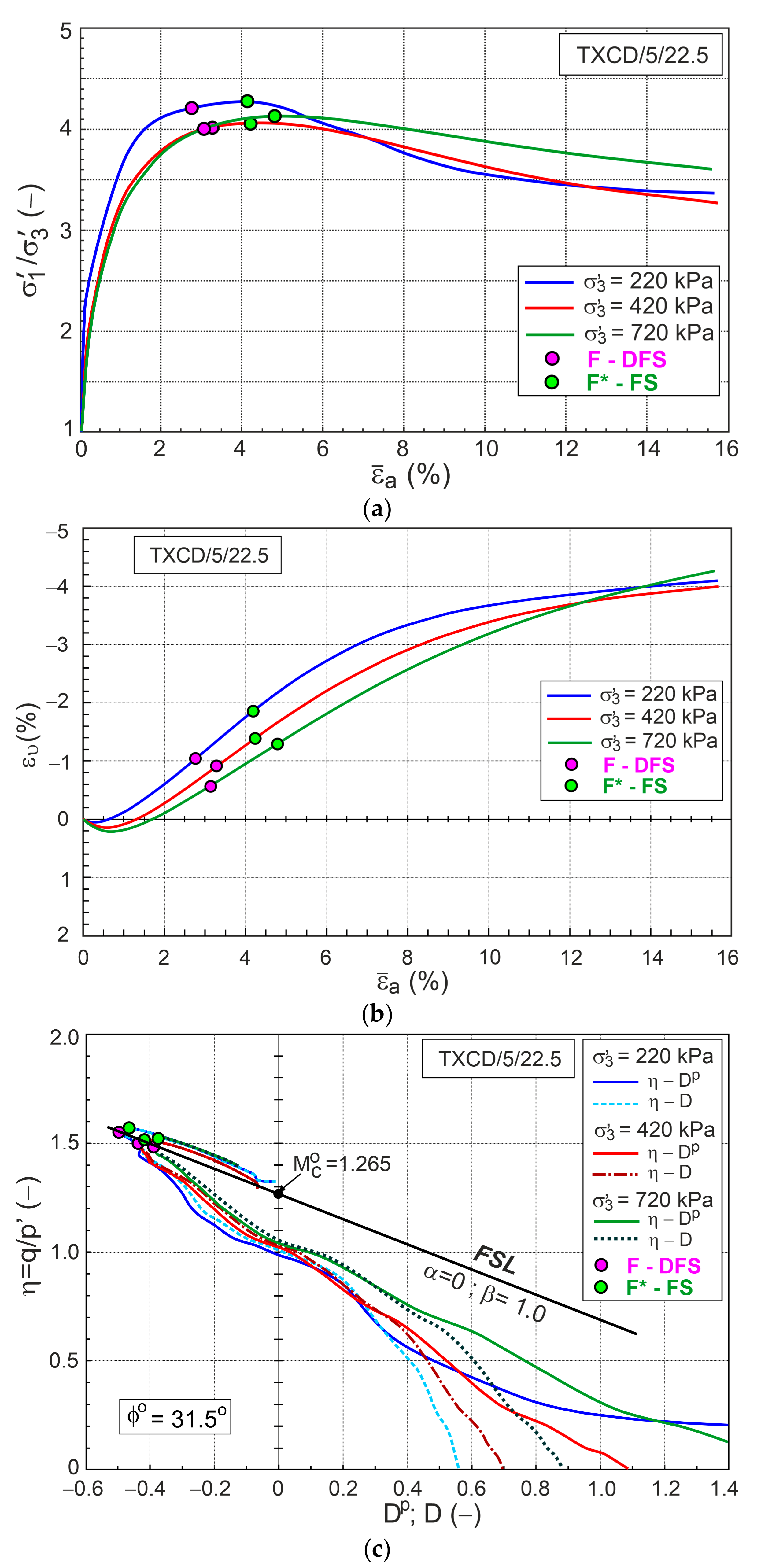
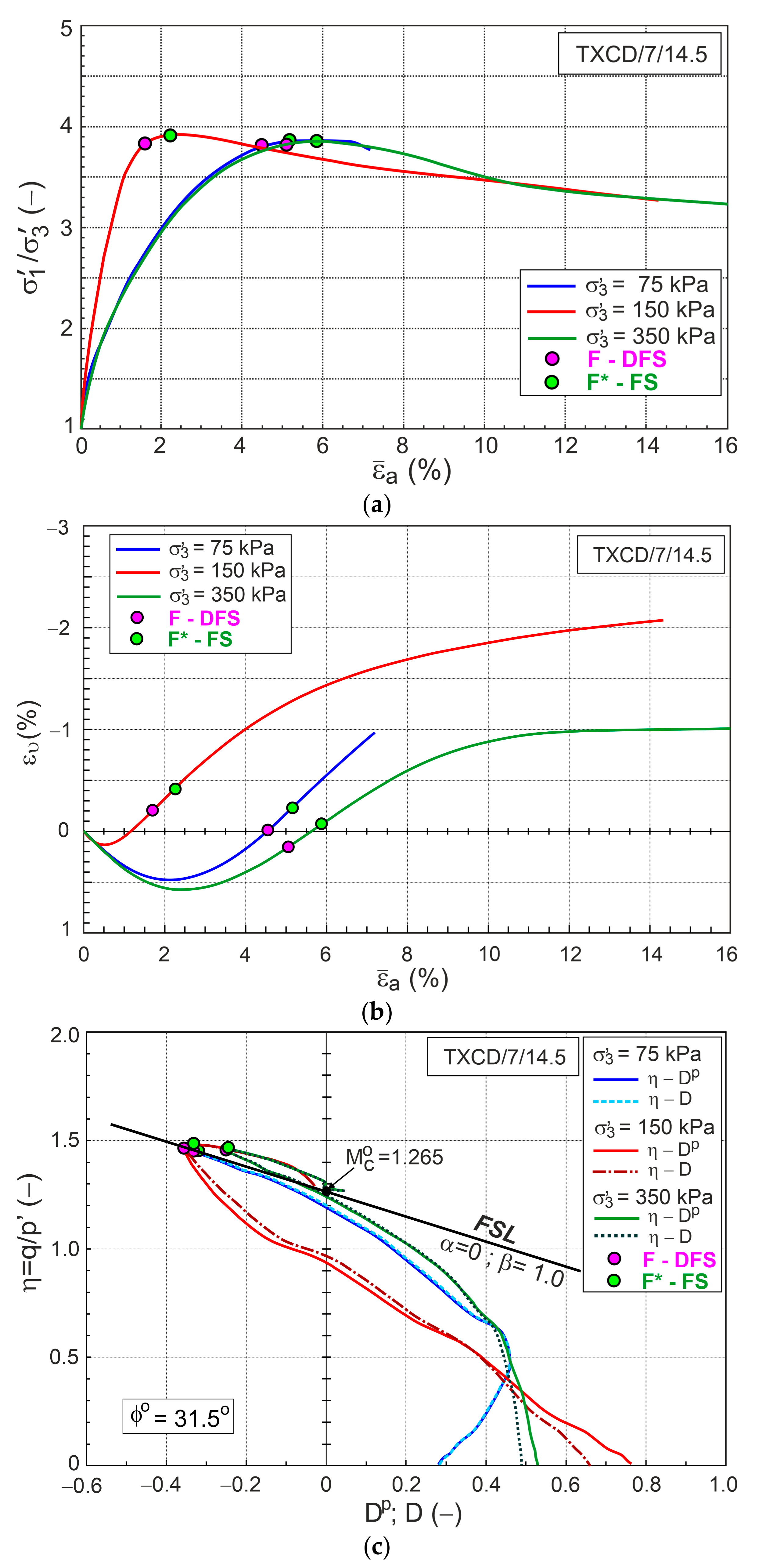
6. Stress Ratio–Plastic Dilatancy Relationship

Figure 4a,b, Figure 5a,b, Figure 6a,b and Figure 7a,b show the ${\sigma }_1^{\prime }/{\sigma }_3^{\prime }-{\overline{\epsilon }}_a$ and ${\epsilon }_{\upsilon }-{\overline{\epsilon }}_a$ relationships traditionally presented in the literature. These relationships are obtained using approximate values of $q$, $p^{\prime }$, and ${\epsilon }_{\upsilon }$. The stress ratio–dilatancy ($\eta -D$) and stress ratio–plastic dilatancy ($\eta -D^p$) relationships are shown in Figure 4c, Figure 5c, Figure 6c and Figure 7c.

The $D^p$ values were calculated using elastic parameters determined by Equations (24)–(27). The differences between $\eta -D$ and $\eta -D^p$ are small for the pre-failure shear stages and do not differ for post-failure shear stages (Figure 4c, Figure 5c, Figure 6c and Figure 7c). The points F representing the DFS in the $\eta -D^p$ plane can be approximated by a straight line called the FSL. For the analyzed drained triaxial compression tests, the FSL is defined by Equation (1) with ${\alpha }_F=0$ and ${\beta }_F=\beta =1.0$; it intersects the vertical axis ($D^p=0$) at $\eta =M_c^o=1.265$, which corresponds to ${\varphi }^o=31.5°$ (Figure 8a).

The $F^{*}$ points represent conventional failure states with the maximum principal stress ratio ${\left({\sigma }_1^{\prime }/{\sigma }_3^{\prime }\right)}_{max}$. The failure states (FSs) can be approximated by the straight failure state line (F*SL) defined by Equation (1), with $M_c^o=1.265$, ${\alpha }_{F*}=0$, and ${\beta }_{F*}=1.138$. For many drained triaxial compression tests presented in the literature for sand, the DFS and FS are equivalent [17]. According to the authors, the difference is influenced by the transverse anisotropy of sand in the tested samples.

The DFS and FS are marked in Figure 4, Figure 5, Figure 6 and Figure 7. These states can be easily identified only in the $\eta -D^p$ plane. The DFS occurred before the FS, before the shear band developed in sheared specimens. Therefore, stresses and strains can be correctly determined for the DFS.

It is worth noting that the FSL is equivalent to the straight line proposed by Bishop [18] for determining the critical state angle (${\varphi }_{cs}$) for sand sheared in conventional drained triaxial compression. Therefore, for sands sheared under low and medium stress levels, ${\varphi }^o={\varphi }_{cs}$. The stress ratio–plastic dilatancy relationship is very helpful in fully describing the behavior of sand (soil) during shearing.

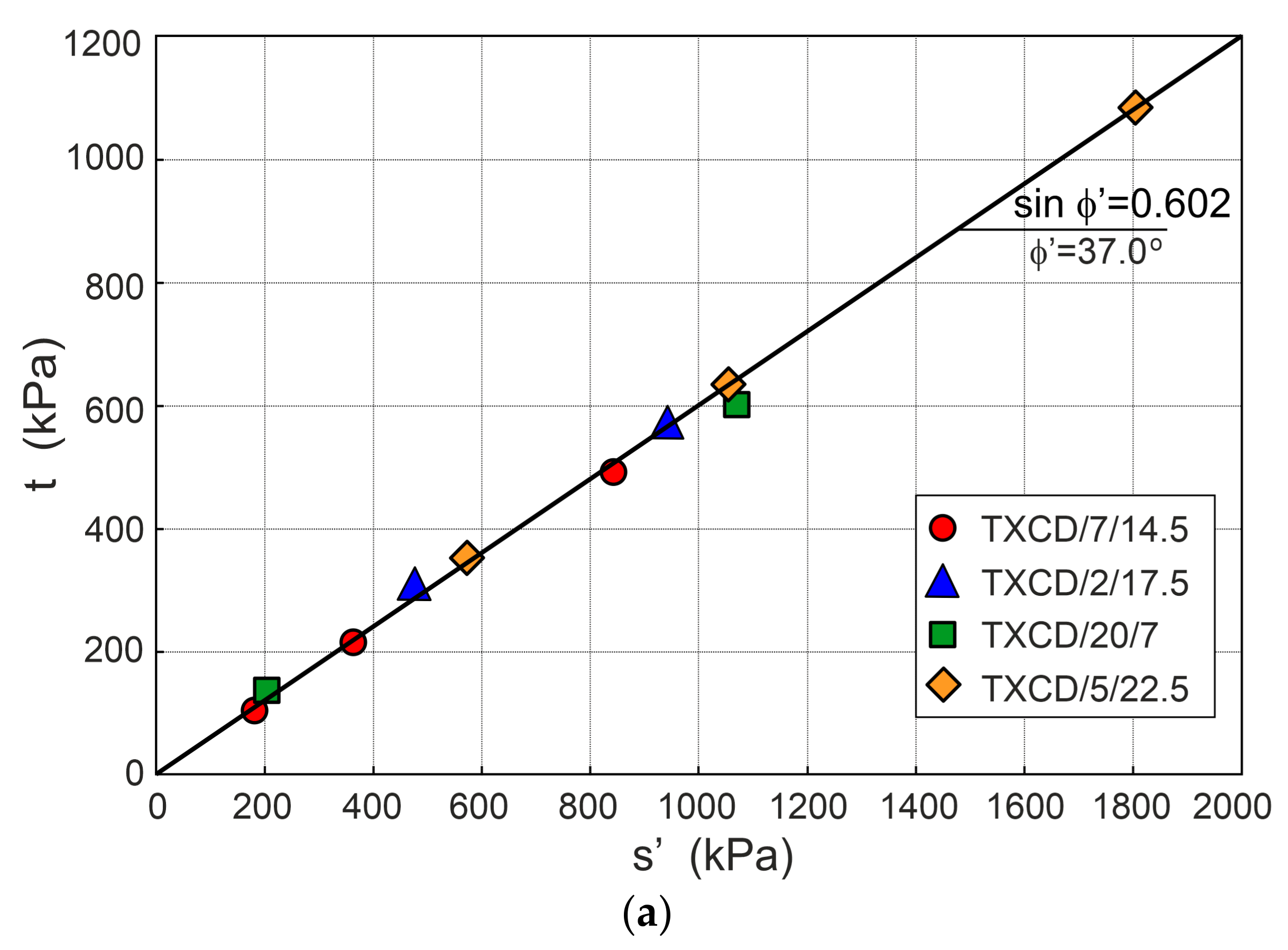
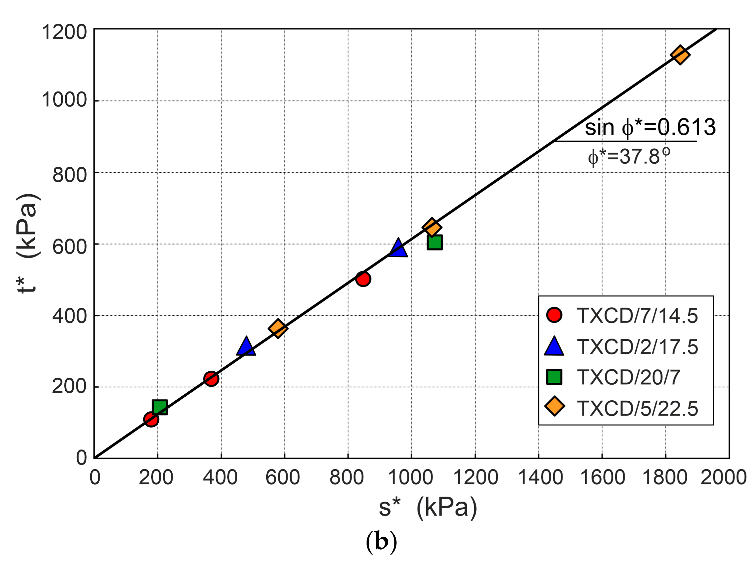
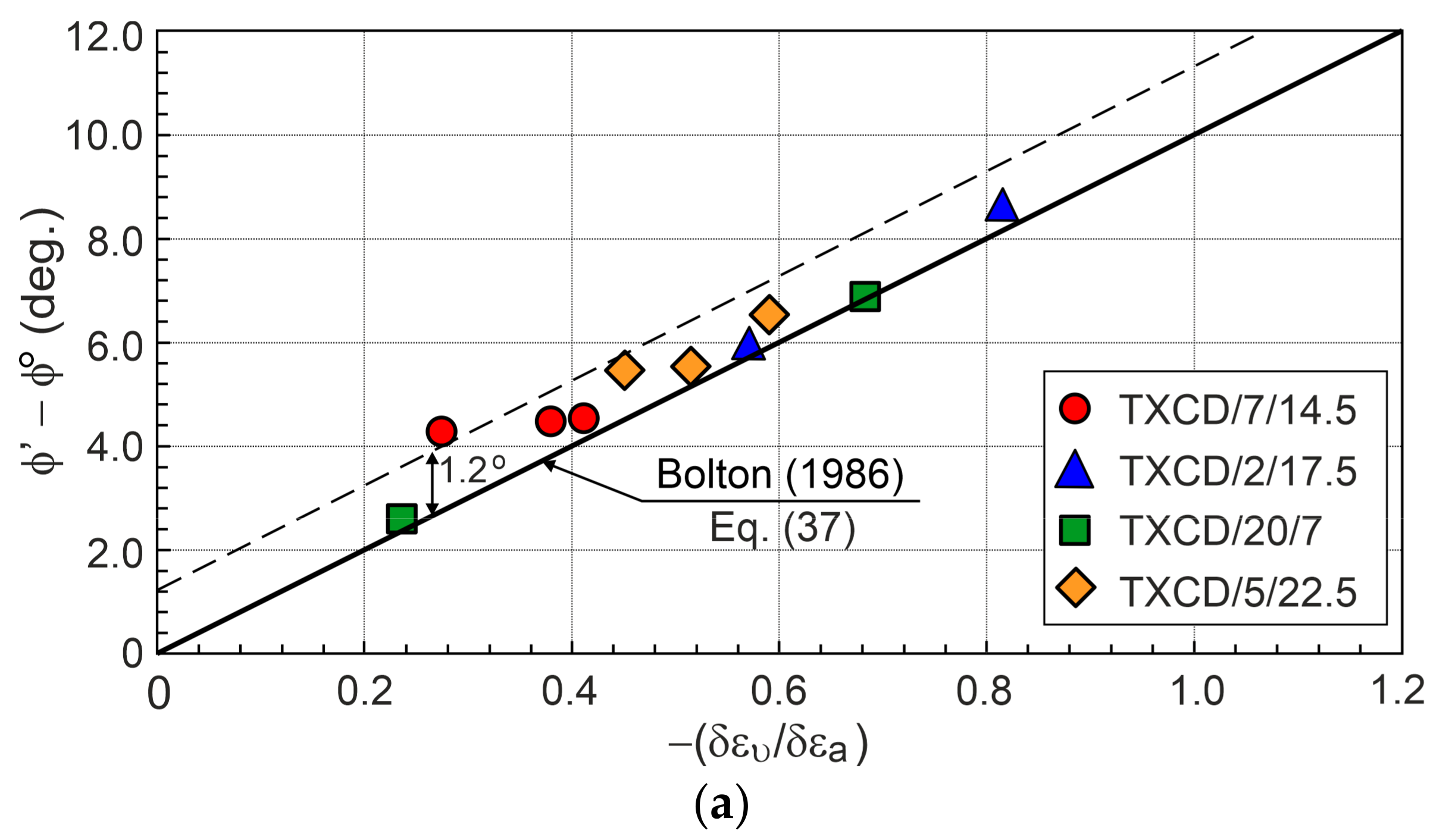
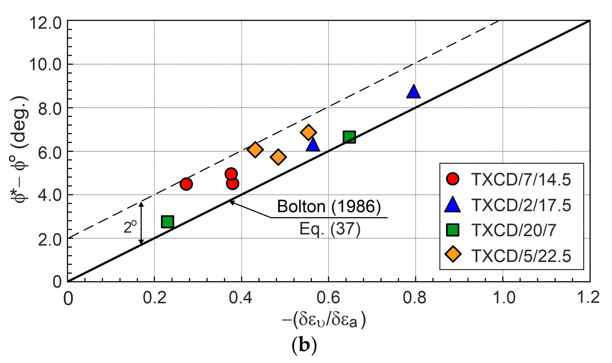
7. Friction Angle of Sand

The effective friction angle of sand can be calculated from the following equation [19]:

$$\sin {\varphi }^{\prime }=t/s^{\prime },$$

(27)

where

$$t={\displaystyle \frac{1}{2}}\left({\sigma }_1^{\prime }-{\sigma }_3^{\prime }\right),$$

(28)

$$s^{\prime }={\displaystyle \frac{1}{2}}\left({\sigma }_1^{\prime }+{\sigma }_3^{\prime }\right).$$

(29)

Equation (27) can have the form

$$\mathit{sin}{\varphi }^{\prime }=\left({\sigma }_1^{\prime }/{\sigma }_3^{\prime }-1\right)/\left({\sigma }_1^{\prime }/{\sigma }_3^{\prime }+1\right).$$

(30)

For triaxial compression,

$${\sigma }_1^{\prime }=p^{\prime }+{\displaystyle \frac{2}{3}}q,$$

(31)

$${\sigma }_3^{\prime }=p^{\prime }-{\displaystyle \frac{1}{3}}q,$$

(32)

$${\sigma }_1^{\prime }/{\sigma }_3^{\prime }=\left(3+2\eta \right)/\left(3-\eta \right),$$

(33)

and

$$\mathit{sin}{\varphi }^{\prime }=3\eta /\left(6+\eta \right).$$

(34)

For the DFS ($\eta ={\eta }_F$), the mean value of $\sin {\varphi }^{\prime }=0.602$ (${\varphi }^{\prime }=37.0°$) (Figure 9a), and for the FS, $\sin {\varphi }^{*}=0.613$ (${\varphi }^{*}=37.8°$) (Figure 9b).

After analyzing data from the drained triaxial compression tests of many sands, Bolton [20] proposed the relationships

$${\varphi }^{\prime }-{\varphi }_{cs}=3I_R,$$

(35)

$${\left(\delta {\epsilon }_{\upsilon }/\delta {\epsilon }_1\right)}_{min}=-0.3I_R,$$

(36)

where $0<I_R<4$ is a sand parameter. For sands, ${\varphi }_{cs}={\varphi }^o$ [18]. Combining Equations (35) and (36) gives the following relationship:

$${\varphi }^{\prime }-{\varphi }^o={-10\left(\delta {\epsilon }_{\upsilon }/\delta {\epsilon }_1\right)}_{min}.$$

(37)

The experimental values ${\varphi }^{\prime }-{\varphi }^o$ for the DFS ${\left(\delta {\epsilon }_{\upsilon }/\delta {\epsilon }_1\right)}_{min}={\left(\delta {\epsilon }_{\upsilon }/\delta {\epsilon }_a\right)}_F$ and the experimental values ${\varphi }^{\mathrm{*}}-{\varphi }^o$ for the FS ${\left(\delta {\epsilon }_{\upsilon }/\delta {\epsilon }_1\right)}_{min}={\left(\delta {\epsilon }_{\upsilon }/\delta {\epsilon }_a\right)}_{F\mathrm{*}}$ are shown in Figure 10a and Figure 10b, respectively.

All experimental values of friction angles are larger than those calculated from Bolton’s equation (Equation (37)). The maximum difference for the DFS is 1.2° (Figure 10a), and it is 2° for the FS (Figure 10b). The stress ratio–plastic dilatancy equation (1) obtained from the FSC well describes the relationship $\left({\varphi }^{\prime }-{\varphi }^o\right)-\left({\delta \epsilon }_{\upsilon }/{\delta \epsilon }_a\right)$ for the DFS, and Bolton’s experimental relation (37) can be treated as an approximation of this relation. In the authors’ opinion, the differences are affected by the transverse anisotropy of sand in the tested sample due to the sample preparation method and small differences between the DFS and FS.

8. Conclusions

(1)

The FSC offers new possibilities for describing the stress–dilatancy behavior of soils (sands).

(2)

The elastic parameters of sand identified from drained triaxial compression tests are lower than those obtained from wave propagation analysis.

(3)

The dilatant failure state and failure state are different for the tested sands. These states can be easily identified in the stress ratio–plastic dilatancy relationships.

(4)

The effective friction angles of the tested sands for the dilatant failure state and failure state are slightly greater than those obtained from Bolton’s formula.

(5)

The deviation in the experimental stress ratio–plastic dilatancy relations from the straight line representing dilatant failure states expresses the combined experimental errors of stress and strain measurements and verifies the quality of experiments.

(6)

The stress ratio–plastic dilatancy relationship obtained from the FSC is important for a complete description of the stress–strain behavior of soils and can be directly used to define the plastic potential function in the elastoplastic modeling of sands.

References

1. Rahimi, M. Review of proposed stress-dilatancy relationships and plastic potential functions for uncemented and cemented sands. J. Geol. Res. 2019, 1, 19–34. [Google Scholar] [CrossRef]
2. Li, X.; Zhu, H.; Yuan, Q. Dilatancy equation based on the property-dependent plastic potential theory for geomaterials. Fractal Fract. 2023, 7, 824. [Google Scholar] [CrossRef]
3. Wood, D.M. Soil Behaviour and Critical State Soil Mechanics, 1st ed.; Cambridge University Press: Cambridge, UK, 1990. [Google Scholar]
4. Schofield, A.N.; Wroth, C.P. Critical State Soil Mechanics; Mc-Grow-Hill Book, Co.: London, UK, 1968. [Google Scholar]
5. Le, L.A.; Nguyen, G.D.; Bui, H.H.; Andrade, J.E. Localised failure of geomaterials: How to extract localisation band behaviour from macro test data. Géotechnique 2022, 72, 569–609. [Google Scholar] [CrossRef]
6. Li, L.; Li, P.; Cai, Y.; Lu, Y. Visualization of non-uniform soil deformation during triaxial testing. Acta Geotech. 2021, 16, 3439–3454. [Google Scholar] [CrossRef]
7. Wan, R.G.; Guo, P.J. Stress dilatancy and fabric dependencies on sand behaviour. J. Eng. Mech. 2004, 130, 635–645. [Google Scholar] [CrossRef]
8. Desrues, J.; Andò, E. Strain localization in granular media. C. R. Phys. 2015, 16, 26–36. [Google Scholar] [CrossRef]
9. Dong, T.; Kong, L.; Zhe, M.; Zheng, Y. Anisotropic failure criterion for soils based on equivalent stress tensor. Soils Found. 2019, 59, 644–656. [Google Scholar] [CrossRef]
10. Liang, J.; Ma, C.; Su, Y.; Lu, D.; Du, X. A failure criterion incorporating the effect of depositional angle for transversely isotropic soils. Comput. Geotech. 2022, 148, 104812. [Google Scholar] [CrossRef]
11. Szypcio, Z. Stress-dilatancy behaviour of calcareous sand. In Proceedings of the 8th International Symposium on Deformation Characteristic of Geomaterials (ISDCG2023), Porto, Portugal, 3–6 September 2023; Available online: https://www.issmge.org/publications/publication/stress-dilatancy-behaviour-of-calcareous-sands (accessed on 4 February 2024).
12. Lambe, W.T.; Whitman, R.V. Soil Mechanics; John Wiley & Sons: New York, NY, USA, 1969. [Google Scholar]
13. Head, K.H.; Epps, R.J. Manual of Soil Laboratory Testing. Vol. III Effective Stress Tests, 3rd ed.; Whittles Publishing: London, UK, 2014. [Google Scholar]
14. Liu, T.; Ferreira, P.M.V.; Vinck, K.; Coop, M.R.; Jardine, R.J.; Kontoe, S. The behaviour of a low- to medium-density chalk under a wide range of pressure conditions. Soils Found 2023, 63, 101268. [Google Scholar] [CrossRef]
15. Gabryś, K.; Dołżyk-Szypcio, K.; Szypcio, Z.; Sas, W. Stress-strain behavior of crushed concrete as a special anthropogenic soil. Materials 2023, 16, 7381. [Google Scholar] [CrossRef] [PubMed]
16. Hardin, B.O.; Richart, F.E. Elastic wave velocities in granular soils. J. Soil Mech. Found. Div. 1963, 89, 33–65. [Google Scholar] [CrossRef]
17. Dołżyk-Szypcio, K. Stressv-dilatancy relationship of Erksak sand under drained triaxial compression. Geosciences 2020, 10, 353. [Google Scholar] [CrossRef]
18. Bishop, A.W. Shear strength parameters for undisturbed and remoulded soil specimens. In Proceedings of the Roscoe Memorial Symposium on Stress-Strain Behaviour of Soils, Cambridge, UK, 29–31 March 1971; Parry, R.H.G., Rosco, K.H., Eds.; G.T. Foulis & Co.: Oxfordshire, UK; pp. 3–58. [Google Scholar]
19. Aysen, A. Soil Mechanics: Basic Concepts and Engineering Applications; Taylor & Francis Group: London, UK, 2005. [Google Scholar]
20. Bolton, M.D. The strength and dilatancy of sands. Géotechnique 1986, 36, 65–68. [Google Scholar] [CrossRef]
Figure 1. Particle size distribution curves of the soils used in this study.
Applsci 14 06228 g001
Figure 2. Instability region for TXC 7/14.5 test: (a) q ε a ; (b) p ε a ; (c) ε υ ε a .
Applsci 14 06228 g002
Figure 3. The shear and bulk moduli of the tested sand: (a) G a p p r G ; (b) K a p p r K .
Applsci 14 06228 g003
Figure 4. Relationships for sample TXC 2/17.5: (a) σ 1 / σ 3 ε ¯ a ; (b) ε υ ε ¯ a ; (c) η D and η D p .
Applsci 14 06228 g004
Figure 5. Relationships for sample TXC 5/22.5: (a) σ 1 / σ 3 ε ¯ a ; (b) ε υ ε ¯ a ; (c) η D and η D p .
Applsci 14 06228 g005
Figure 6. Relationships for sample TXC 7/14.5: (a) σ 1 / σ 3 ε ¯ a ; (b) ε υ ε ¯ a ; (c) η D and η D p .
Applsci 14 06228 g006
Figure 7. Relationships for sample TXC 20/7: (a) σ 1 / σ 3 ε ¯ a ; (b) ε υ ε ¯ a ; (c) η D and η D p .
Applsci 14 06228 g007
Figure 8. The η D p relationships for (a) DFS and (b) FS.
Applsci 14 06228 g008
Figure 9. Effective friction angle of sand for (a) DFS and (b) FS.
Applsci 14 06228 g009aApplsci 14 06228 g009b
Figure 10. The difference between the effective friction angle and the critical frictional state angle for (a) DFS and (b) FS.
Applsci 14 06228 g010aApplsci 14 06228 g010b